| Issue |
A&A
Volume 653, September 2021
|
|
|---|---|---|
| Article Number | L10 | |
| Number of page(s) | 6 | |
| Section | Letters to the Editor | |
| DOI | https://doi.org/10.1051/0004-6361/202039033 | |
| Published online | 24 September 2021 | |
Letter to the Editor
Extremely weak CO emission in IZw 18
1
School of Astronomy and Space Science, Nanjing University, Nanjing 210093, PR China
e-mail: wenjia@nju.edu.cn, yshipku@gmail.com
2
Key Laboratory of Modern Astronomy and Astrophysics (Nanjing University), Ministry of Education, Nanjing 210093, PR China
3
Shanghai Astronomical Observatory, Chinese Academy of Sciences, 80 Nandan Road, Shanghai 200030, PR China
Received:
26
July
2020
Accepted:
9
September
2021
Local metal-poor galaxies are ideal analogues of primordial galaxies with the interstellar medium (ISM) barely being enriched with metals. However, it is unclear whether carbon monoxide remains a good tracer and coolant of molecular gas at low metallicity. Based on the observation with the upgraded Northern Extended Millimeter Array, we report a marginal detection of CO J = 2–1 emission in IZw18, pushing the detection limit down to L′CO(2-1) = 3.99 × 10³ K km s−1 pc−2, which is at least 40 times lower than previous studies. As one of the most metal-poor galaxies, IZw18 shows extremely low CO content despite its vigorous star formation activity. Such low CO content relative to its infrared luminosity, star formation rate, and [C II] luminosity, compared with other galaxies, indicates a significant change in the ISM properties at a few percent of the Solar metallicity. In particular, the high [C II] luminosity relative to CO implies a larger molecular reservoir than the CO emitter in IZw18. We also obtain an upper limit of the 1.3 mm continuum, which excludes a sub-millimetre excess in IZw18.
Key words: galaxies: dwarf / ISM: molecules
© ESO 2021
1. Introduction
Star formation occurs in molecular gas dominated by H2, except perhaps for the star formation in the early universe. However, H2 can only be excited at a temperature above 100 K, hence it cannot be observed directly in the cold molecular gas that fuels star formation. The second most abundant molecule, CO, has been demonstrated to be a powerful tracer of molecular clouds in galaxies, but this application becomes complicated in metal-poor environments (see Bolatto et al. 2013, for a review).
In the early Universe, the first galaxies formed in the primordial gas with few elements being heavier than hydrogen. Observationally, at z ≳ 5, normal star-forming galaxies with star formation rates (SFRs) of ten to a few hundred solar masses per year indeed have a low dust content (Walter et al. 2012; Capak et al. 2015), comparable to local metal-poor galaxies. Nevertheless, the predicted CO flux in these high-z galaxies is of the order of μJy and remains challenging due to the state-of-the-art sub-millimetre array, Atacama Large Millimeter/submillimeter Array (ALMA). A detailed study on the metal-poor interstellar medium (ISM) relies on its local analogues.
Despite the extensive search for CO emissions in local dwarf galaxies (Leroy et al. 2007; Schruba et al. 2012; Cormier et al. 2014; Hunt et al. 2015; Warren et al. 2015; Shi et al. 2015), the detection rate decreases sharply in galaxies with a metallicity lower than one-fifth the Solar metallicity (Z⊙)1. The extremely faint CO emission brings about questions as to the existence of molecular gas in such galaxies. On the other hand, CO may not be an ideal tracer of molecular gas (Grenier et al. 2005; Wolfire et al. 2010; Shi et al. 2016) in low-metallicity environments. The interstellar radiation penetrates deeper into molecular clouds due to the low dust content. At such depths within the clouds, CO is more easily destroyed than H2 through dissociation, and thus it ceases to be a reliable tracer. In addition, the reduced opacity in the stellar atmosphere leads to harder radiation fields, and hence reinforces the destruction of CO molecules into atomic or singly ionised carbon.
Low CO content is then expected in metal-poor galaxies. On the other hand, exposed to the hard radiation field, CO molecules can be easily photodissociated and produce ionised carbon, [C II]. Furthermore, [C II] could come from ionised gas as well as neutral gas and the surface of photodissociation regions (PDRs). However, the fractions of [C II] emission from ionised gas derived from observation constraints are systematically lower than the one from simulations (Accurso et al. 2017b; Cormier et al. 2019). Therefore it is still unclear whether it is feasible to use [C II] to trace H2 gas.
Substantial efforts have been made to search for the molecular gas in metal-poor galaxies (Rubio et al. 2015; Oey et al. 2017; Schruba et al. 2017; Elmegreen et al. 2018); nevertheless, among the galaxies below 10% Z⊙, only Sextans B (7% Z⊙) has a robust CO detection (Shi et al. 2016, 2020). The impact of low metal abundance on star formation requires further exploration of the most metal-poor galaxies. In this work, we used the upgraded NOEMA interferometer to observe the CO J = 2–1 emission in IZw18, which is one of the galaxies with the lowest metallicities in the local Universe (∼3% Z⊙, Izotov & Thuan 1999). IZw18 is a proto-type of blue compact dwarfs located at a distance of 18.2 Mpc (Aloisi et al. 2007). The active star formation therein (Hunt et al. 2005) indicates the presence of molecular gas. Leroy et al. (2007) obtained an upper limit of CO(1–0) emission ( < 105 K km s−1 pc2) using the Plateau de Bure Interferometer (PdBI), which however is not deep enough to conclude whether IZw 18 has a normal CO content relative to other physical properties. Here we put further constraints on the CO content in IZw18 by pushing down the detection limit of
  by 40 times using the Northern Extended Millimeter Array (NOEMA) after its Phase II upgrade.
2. Observations
The observations of IZw18 were carried out with NOEMA on December 24, 2017 (obs-17) and March 23, 2019 (obs-19) for a total of 16 h (11.6 h on source) with configuration D. We processed the data at IRAM/Grenoble using the GILDAS package. The final CO J = 2–1 datacubes of obs17, obs18, and the merger of the two have beam sizes of 1 83 × 1
 60 (obs-17), 1
 71 × 1
 41 (obs-18), and 1
 71 × 1
 48 (merged), respectively, and a frequency resolution of 0.2 MHz (0.26 km s−1 at 230 GHz). IZw18 was entirely covered by the 22″ (FWHM) primary beam. The details of the observation settings and the sensitivities of the data are listed in Table 1.
Observation information.
3. Results
3.1. CO J = 2–1
We smoothed the data to a velocity resolution of 3 km s−1, consistent with the CO line width found in the most metal-poor galaxies in the literature (Shi et al. 2016). We found one marginal detection (α = 9h34m02s00, δ = 55°14′28 81) at the peak of the stellar emission, as indicated by the red contour2 superimposed on the Hubble Space Telescope (HST) V-band image (Fig. 1)3. It covers an area defined by the 3σ contour of ∼1
 52 × 1
 52, which is approximately the size of the synthesised beam. We have plotted the spectra from the merged, obs-17 and obs-19 data cubes in Fig. 2. A 3σ spectral signal falls at 46 km s−1. The peak fluxes derived from the peak channels have signal-to-noise ratios of 3.47, 2.73, and 3.45 for the merged, obs-17 and obs-19 data cubes. We note that even though the spectrum extracted from the obs-17 data cube shows lower rms noise, the noise level in the data cube slightly deviates from a Gaussian distribution, while those from obs-19 and merged data cubes do not. Hereafter, we use the result from the merged data cube.
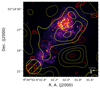 |
Fig. 1. CO J = 2–1 emission and 1.3 mm continuum superimposed on the HST V-band image from Izotov & Thuan (2004, PropID: 9400). The red contours denote the CO J = 2–1 integrated line intensity at the resolution of 1 |


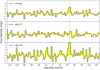 |
Fig. 2. CO J = 2–1 spectra from the merged, obs-17 and obs-19 data cubes. The spectra are smoothed to a velocity resolution of 3 km s−1 and extracted from the area defined by the 3σ contour as shown in Fig. 1. The 1σ uncertainty is 0.72, 0.72, and 1.39 mJy, respectively. The grey dashed line denotes the marginal detection at ∼46 km s−1. |
The CO J = 2–1 peak flux density is SCO(2−1) = 2.48 mJy and the corresponding CO luminosity is then derived to be  = 3.99 × 10³ K km s−1 pc−2 using the formulation of Solomon & Vanden Bout (2005). The CO emission tends to reside in clumps of a few parsecs at low metallicity (Rubio et al. 2015; Oey et al. 2017; Schruba et al. 2017; Shi et al. 2020), which is much smaller than the beam size of our observation, hence we do not expect significant missing diffuse emission.
3.2. 1.3 mm continuum
We created a continuum map after removing channels with emission. The continuum map was smoothed to have an angular resolution of 2 21 × 2
 06 with an rms noise of 51 μJy beam−1, using the TCLEAN TASK IN CASA. The flux peak falls at α = 9h34m02s00, δ = 55°14′26
 30 which is between the two flux peaks of the H I emission of IZw18 (Lelli et al. 2012, see also Appendix A). This is the only 3σ signal (F1.3 mm = 181 μJy) within the primary beam. Comparisons between CO J = 2–1 emission and 1.3 mm continuum as well as the emission at FUV, 3.6 μm, 24 μm, 100 μm, and of H I gas are shown in Appendix A.
4. Discussion
In this section, we discuss how the CO luminosity and the 1.3 mm continuum flux constrain our current understanding of the star formation process in the extremely metal-poor environment in IZw18. The physical parameters we used for IZw18 are listed in Table 2.
Basic information on IZw18 used in this paper.
We compare IZw18 to normal star-formimg galaxies and metal-poor galaxies in the literature. These include seven metal-poor dwarf galaxies from the Herschel Dwarf Galaxy Survey (DGS, Cormier et al. 2014, compiled in Accurso et al. 2017b), 16 nearby dwarf galaxies in Schruba et al. (2012) and nearby galaxies compiled therein, eight metal-poor galaxies from Hunt et al. (2015), local galaxies with stellar mass higher than 109 M⊙ from the xCOLD GASS survey (Saintonge et al. 2017), and massive, infrared bright, local star-forming galaxies at Solar metallicity from Gao & Solomon (2004), as well as the individual star-forming regions in four extremely metal-poor galaxies (12 + log (O/H) < 8) from Shi et al. (2015, 2016).
4.1. SED and sub-millimetre excess
We first investigated the spectral energy distribution (SED) of IZw18 taking into account the 3σ upper limit at 1.3 mm to put more constraints on the FIR/millimetre regime. All other photometric data were taken from Hunt et al. (2014). We performed the SED fitting with CIGALE (Boquien et al. 2019) adopting a delayed star formation history, a Draine & Li (2007) dust model, which is consistent with the method used for the star-forming regions in Shi et al. (2015, 2016), and a radio component. The infrared luminosity derived from the fit is 2.2 × 10⁷ L⊙, consistent with the one from Hunt et al. (2014). The stellar mass is 4.33 × 10⁶ M⊙, within the uncertainty of the stellar masses derived from stellar mass-to-light ratios in the K band and 3.6 μm (Fumagalli et al. 2010; Hunt et al. 2019), while it is around ten times lower than those derived based on the R band luminosity (Lelli et al. 2012, 2014).
We also explored the existence of the excess at sub-millimeter wavelengths (e.g., Galliano et al. 2003; Lisenfeld et al. 2002; Galametz et al. 2011; Rémy-Ruyer et al. 2013) in IZw18. It did not have a robust detection at the far-infrared (FIR) wavelengths longer than 160 μm. The 3σ upper limit at 1.3 mm places a strong constraint on the (sub-) millimetre end of the dust emission. We fitted the FIR SED with the modified blackbody model and derived a lower limit of the dust emissivity β to be 2.1, which suggests no sub-millimetre excess in IZw18. Furthermore, taking into account the upper limit at 1.3 mm, we notice that the radio emission shows a steeper slope (α = −0.58), compared to the spectral indice found in Hunt et al. (2005) ( = −0.39,
  = −0.13); this may be due to the high frequency cutoff of synchrotron emission from the relavitistic electrons in the star-forming regions. Therefore, we fitted the radio emission with a cutoff model as introduced in Klein et al. (2018), by fixing the spectral index of the synchrotron emission to be αnth =
  = −0.39 (Fig. 3). Then the contribution of the free-free emission to the total radio emission is
  ∼ 76% and
  ∼ 54%, higher than what was found in the literature (e.g. Leroy et al. 2007; Hunt et al. 2014). We note that the cutoff frequency derived from the fit is at 145 GHz, which is higher than the typical value of ∼10 GHz found in Klein et al. (2018).
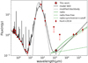 |
Fig. 3. SED of IZw18, with CIGALE best fit adopting a delayed star formation history, a Draine & Li (2007) dust model, and a radio component. A modified blackbody fit is shown with a grey line. Photometric data are from Hunt et al. (2014), except for at 1.3 mm. The 3σ upper limit at 1.3 mm is shown as in the red star. The radio emission is also fitted with a cutoff model including a free-free component and a synchrotron component as introduced in Klein et al. (2018) (see more in the Sect. 4.1), which is indicated by the green curves. |
4.2. LIR and SFR versus 
In Fig. 4, we have plotted the total infrared luminosity (8–1000 μm), LIR, versus  and the SFR versus
  . These two correlations have been well established in massive star-forming galaxies (e.g. Gao & Solomon 2004) as CO molecules and LIR trace H2 molecular clouds and dust emission, respectively. We assume optically thick and thermalised CO emission, then
  =
=  . We note that CO tends to become warm and optically thin as CO is exposed to interstellar radiation in metal-poor galaxies. Schruba et al. (2012) adopted R21 = 0.7, which is the average value of HERACLES galaxies (Rosolowsky et al. 2015) for nearby dwarf galaxies. Saintonge et al. (2011) studied the 523 galaxies in xCOLD GASS survey and gave an average value of 0.79±0.03 with a larger scatter at
  < 108 K km s−1 pc2. Therefore, the choice of R21 may lead to the derived
  a factor of 1.4 different from the one based on our assumption. The SFR was derived from the combination of FUV and 24 μm emission for all galaxies, except for the infrared bright galaxies for which the SFR was derived from infrared luminosity.
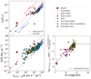 |
Fig. 4. Infrared luminosity (top left) and SFR (derived from the emission at FUV and 24 μm, bottom left) versus |


Compared to star-forming galaxies with Solar metallicity, metal-poor galaxies show higher LIR/ and SFR/
 ratios. The LIR/
 ratio of metal-poor galaxies is, on average, 15.4 times higher than the one of the massive, normal star-forming galaxies at Solar luminosity. IZw18 shows even higher LIR/
 and SFR/
 ratios, which are ≳5.7 and ≳119 times higher than those of other metal-poor galaxies (Fig. 4-Top left), respectively. It is difficult for CO molecules to form in metal-poor environments because there is fewer raw material and little dust to protect the already scarce CO molecules from UV radiation. The higher ratios are a natural result of this. The SFR/
 ratio of metal-poor galaxies increases as the metallicity decreases (Fig. 4-Bottom right). Hunt et al. (2015) found a significant correlation when fitting their dwarf galaxies, detections in Schruba et al. (2012), and the compilation therein. We see a slightly shallower trend when including all galaxies with a CO detection. We kept only the star-forming galaxies in xCOLD in the regression to exclude the contamination from active galactic nucleis. The SFR/
 ratio of IZw18 falls above the trend and it is more than ten times higher than the rest of the galaxies. This suggests a great difference in the CO distribution and content of galaxies similar to IZw18, at a few percentages of solar metallicity, than that of metal-rich galaxies. However, as we discuss below, the change may occur gradually with the decreased metallicity.
SFR and  can be derived from observations, but the molecular gas mass, MH2 = αCO ×
  , is the key quantity of interest. The observed SFR/
 ratio is related to both the depletion time (τdep) and the CO-to-H2 conversion factor (αCO) as SFR/
 = SFR/(MH2/αCO) = αCO/τdep. Many studies have shown that αCO increases rapidly at low metallicity theoretically and observationally (Israel 1997; Glover & Mac Low 2011; Leroy et al. 2011; Narayanan et al. 2012; Elmegreen et al. 2013; Shi et al. 2016). If τdep is constant, as is found for the nearby disc galaxies (Leroy et al. 2008; Bigiel et al. 2011), then the dependence of the SFR/
 ratio on metallicity is the direct consequence of the variation of αCO. However, τdep in dwarf galaxies remains uncertain and tends to be shorter at a lower mass and at a higher specific SFR (sSFR; Saintonge et al. 2011; Shi et al. 2014; Hunt et al. 2020). IZw18, as a dwarf galaxy with a relatively high sSFR and low mass, is likely to have low τdep. We speculates that as αCO = τdep ×
  , the high SFR/
 ratio of IZw18 would overwhelm the possibly low τdep, and this would result in a high αCO. Moreover, considering the dependence of αCO on both sSFR and metallicity for the metal poor galaxies, IZw18 follows the empirical relation found in Hunt et al. (2020) within the uncertainty of the stellar mass, as shown in the bottom right corner of Fig. 5. This relation was derived based on a recent compilation of ∼400 metal poor galaxies (Ginolfi et al. 2020, MAGMA). We note that the individual star-forming regions of the metal-poor galaxies from Shi et al. (2015, 2016) all fall slightly above the relation, but well within the scatter of the global measurements of the galaxies. This indicates that αCO changes continuously with metallicity and sSFR. A further constraint on the conversion factor (αCO) of IZw18 is beyond the scope of this paper.
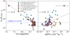 |
Fig. 5. LC II/LCO(1−0) ratio as a function of the metallicity (left) and specific SFR (right). IZw18 (red star) is compared to the galaxies compiled in Zanella et al. (2018, see references therein). The errorbar reflects the uncertainties of stellar mass and SFR. Pearson’s correlation coefficients for the regression fits are shown in each panel. |
4.3. The structure of the interstellar medium
Bolatto et al. (1999) and Röllig et al. (2006) modelled the PDRs and found that as the [C II] regions expand at low metallicity, the L[C II]/LCO(1−0) ratio increases. This has also been confirmed in previous observations (Madden 2000; Cormier et al. 2014). Cormier et al. (2015) detected the bright [C II] emission in IZw18. We plotted the L[C II]/LCO(1−0) ratio as a function of metallicity and specific SFR in Fig. 5. IZw18 generally follows the trend with metallicity, defined by the galaxies compiled by Zanella et al. (2018, see references therein), but it shows ratios several times higher than the prediction of the regression fit to sSFR. We note that [C II] is considered to be a good tracer of CO-dark molecular gas (e.g. Cormier et al. 2015; Accurso et al. 2017b; Zanella et al. 2018; Madden et al. 2020). Even though [C II] can originate from both ionised gas and neutral gas, simulations and models have found that the ionised fraction does not go beyond 50%, even for metal-poor galaxies (Accurso et al. 2017a; Cormier et al. 2019). The ionised fraction of IZw18 is unknown, but it could be low as recent studies found a decreasing fraction with decreasing metallicity (Madden et al. 2020, and references therein). This indicates that the total molecular reservoir, traced by [C II] emission from PDRs, is much larger than the CO emitter in IZw18. Then the extreme case of IZw18 reinforces a significant change in the ISM structure in systems at a few percent of the Solar metallicity and this may have similar implications for such systems in the early Universe.
5. Conclusions
In this Letter, we report a marginal detection of CO J = 2–1 in IZw18, using the observation from NOEMA after its Phase II upgrade. We pushed the detection limit of  down to
  = 3.99 × 10³ K km s−1 pc−2, which is 40 times lower than that of Leroy et al. (2007). As one of the most metal-poor galaxies, IZw18 shows LIR/
 and SFR/
 ratios much higher than those of galaxies with a higher metal abundance. Particularly, the SFR/
 ratio of IZw18 constrains the CO-to-H2 conversion factor to rise considerably at metallicity lower than 5% Z⊙. The SFR/
 ratio also follows the regression found in Hunt et al. (2020) well which considers the influence of both sSFR and metallicity. The high L[C II]/LCO(1−0) ratio indicates that the CO emitter may trace only the inner part of the entire molecular gas reservoir due to the extremely low metallicity of IZw18. An upper limit of the continuum emission at 1.3 mm is also obtained to constrain the Rayleigh Jeans tail of the SED and we excluded a sub-millimetre excess in IZw18.
Here we adopt Solar metallicity as 12 + log(O/H) = 8.7 (Asplund et al. 2009).
The red contours show the CO J = 2–1 line intensity integrated from 40 km s−1 to 50 km s−1, where the marginal detection falls, as shown in Fig. 2.
Acknowledgments
We are grateful to the referee for useful comments which significantly improved the quality of this manuscript. L. Z. and Y. S. acknowledge the support from the National Key R&D Program of China (No. 2018YFA0404502, No. 2017YFA0402704) and the National Natural Science Foundation of China (NSFC grants 11825302, 11733002 and 11773013) and the science research grants from the China Manned Space Project with NO. CMS-CSST-2021-B02. Y. S. thanks the support by the Tencent Foundation through the XPLORER PRIZE. L. Z. also acknowledges China Scholarship Council (CSC). J. W. is thankful for the support of NSFC (grant 11590783). Z. Y. Z. acknowledges the support of NSFC (grant 12041305) and the Program for Innovative Talents, Entrepreneur in Jiangsu.
References
- Accurso, G., Saintonge, A., Catinella, B., et al. 2017a, MNRAS, 470, 4750 [NASA ADS] [Google Scholar]
- Accurso, G., Saintonge, A., Bisbas, T. G., & Viti, S. 2017b, MNRAS, 464, 3315 [NASA ADS] [CrossRef] [Google Scholar]
- Aloisi, A., Clementini, G., Tosi, M., et al. 2007, ApJ, 667, L151 [NASA ADS] [CrossRef] [Google Scholar]
- Asplund, M., Grevesse, N., Sauval, A. J., & Scott, P. 2009, ARA&A, 47, 481 [NASA ADS] [CrossRef] [Google Scholar]
- Bigiel, F., Leroy, A. K., Walter, F., et al. 2011, ApJ, 730, L13 [NASA ADS] [CrossRef] [Google Scholar]
- Bolatto, A. D., Jackson, J. M., & Ingalls, J. G. 1999, ApJ, 513, 275 [NASA ADS] [CrossRef] [Google Scholar]
- Bolatto, A. D., Wolfire, M., & Leroy, A. K. 2013, ARA&A, 51, 207 [CrossRef] [Google Scholar]
- Boquien, M., Burgarella, D., Roehlly, Y., et al. 2019, A&A, 622, A103 [NASA ADS] [CrossRef] [EDP Sciences] [Google Scholar]
- Brown, M. J. I., Moustakas, J., Smith, J. D. T., et al. 2014, ApJS, 212, 18 [Google Scholar]
- Capak, P. L., Carilli, C., Jones, G., et al. 2015, Nature, 522, 455 [NASA ADS] [CrossRef] [Google Scholar]
- Cormier, D., Madden, S. C., Lebouteiller, V., et al. 2014, A&A, 564, A121 [NASA ADS] [CrossRef] [EDP Sciences] [Google Scholar]
- Cormier, D., Madden, S. C., Lebouteiller, V., et al. 2015, A&A, 578, A53 [NASA ADS] [CrossRef] [EDP Sciences] [Google Scholar]
- Cormier, D., Abel, N. P., Hony, S., et al. 2019, A&A, 626, A23 [NASA ADS] [CrossRef] [EDP Sciences] [Google Scholar]
- Draine, B. T., & Li, A. 2007, ApJ, 657, 810 [NASA ADS] [CrossRef] [Google Scholar]
- Elmegreen, B. G., Rubio, M., Hunter, D. A., et al. 2013, Nature, 495, 487 [NASA ADS] [CrossRef] [Google Scholar]
- Elmegreen, B. G., Herrera, C., Rubio, M., et al. 2018, ApJ, 859, L22 [NASA ADS] [CrossRef] [Google Scholar]
- Fisher, D. B., Bolatto, A. D., Herrera-Camus, R., et al. 2014, Nature, 505, 186 [NASA ADS] [CrossRef] [Google Scholar]
- Fumagalli, M., Krumholz, M. R., & Hunt, L. K. 2010, ApJ, 722, 919 [NASA ADS] [CrossRef] [Google Scholar]
- Galametz, M., Madden, S. C., Galliano, F., et al. 2011, A&A, 532, A56 [NASA ADS] [CrossRef] [EDP Sciences] [Google Scholar]
- Galliano, F., Madden, S. C., Jones, A. P., et al. 2003, A&A, 407, 159 [NASA ADS] [CrossRef] [EDP Sciences] [Google Scholar]
- Gao, Y., & Solomon, P. M. 2004, ApJ, 606, 271 [NASA ADS] [CrossRef] [Google Scholar]
- Gil de Paz, A., Madore, B. F., & Pevunova, O. 2003, ApJS, 147, 29 [NASA ADS] [CrossRef] [Google Scholar]
- Gil de Paz, A., Boissier, S., Madore, B. F., et al. 2007, ApJS, 173, 185 [Google Scholar]
- Ginolfi, M., Hunt, L. K., Tortora, C., Schneider, R., & Cresci, G. 2020, A&A, 638, A4 [CrossRef] [EDP Sciences] [Google Scholar]
- Glover, S. C. O., & Mac Low, M. M. 2011, MNRAS, 412, 337 [NASA ADS] [CrossRef] [MathSciNet] [Google Scholar]
- Grenier, I. A., Casandjian, J.-M., & Terrier, R. 2005, Science, 307, 1292 [Google Scholar]
- Hunt, L. K., Dyer, K. K., & Thuan, T. X. 2005, A&A, 436, 837 [NASA ADS] [CrossRef] [EDP Sciences] [Google Scholar]
- Hunt, L. K., Testi, L., Casasola, V., et al. 2014, A&A, 561, A49 [NASA ADS] [CrossRef] [EDP Sciences] [Google Scholar]
- Hunt, L. K., García-Burillo, S., Casasola, V., et al. 2015, A&A, 583, A114 [NASA ADS] [CrossRef] [EDP Sciences] [Google Scholar]
- Hunt, L. K., De Looze, I., Boquien, M., et al. 2019, A&A, 621, A51 [NASA ADS] [CrossRef] [EDP Sciences] [Google Scholar]
- Hunt, L. K., Tortora, C., Ginolfi, M., & Schneider, R. 2020, A&A, 643, A180 [CrossRef] [EDP Sciences] [Google Scholar]
- Israel, F. P. 1997, A&A, 328, 471 [NASA ADS] [Google Scholar]
- Izotov, Y. I., & Thuan, T. X. 1999, ApJ, 511, 639 [NASA ADS] [CrossRef] [Google Scholar]
- Izotov, Y. I., & Thuan, T. X. 2004, ApJ, 616, 768 [CrossRef] [Google Scholar]
- Klein, U., Lisenfeld, U., & Verley, S. 2018, A&A, 611, A55 [NASA ADS] [CrossRef] [EDP Sciences] [Google Scholar]
- Lelli, F., Verheijen, M., Fraternali, F., & Sancisi, R. 2012, A&A, 537, A72 [NASA ADS] [CrossRef] [EDP Sciences] [Google Scholar]
- Lelli, F., Verheijen, M., & Fraternali, F. 2014, MNRAS, 445, 1694 [Google Scholar]
- Leroy, A., Cannon, J., Walter, F., Bolatto, A., & Weiss, A. 2007, ApJ, 663, 990 [NASA ADS] [CrossRef] [MathSciNet] [Google Scholar]
- Leroy, A. K., Walter, F., Brinks, E., et al. 2008, AJ, 136, 2782 [Google Scholar]
- Leroy, A. K., Bolatto, A., Gordon, K., et al. 2011, ApJ, 737, 12 [Google Scholar]
- Lisenfeld, U., Israel, F. P., Stil, J. M., & Sievers, A. 2002, A&A, 382, 860 [NASA ADS] [CrossRef] [EDP Sciences] [Google Scholar]
- Madden, S. C. 2000, New Astron. Rev., 44, 249 [Google Scholar]
- Madden, S. C., Cormier, D., Hony, S., et al. 2020, A&A, 643, A141 [CrossRef] [EDP Sciences] [Google Scholar]
- Narayanan, D., Krumholz, M. R., Ostriker, E. C., & Hernquist, L. 2012, MNRAS, 421, 3127 [NASA ADS] [CrossRef] [Google Scholar]
- Oey, M. S., Herrera, C. N., Silich, S., et al. 2017, ApJ, 849, L1 [NASA ADS] [CrossRef] [Google Scholar]
- Rémy-Ruyer, A., Madden, S. C., Galliano, F., et al. 2013, A&A, 557, A95 [NASA ADS] [CrossRef] [EDP Sciences] [Google Scholar]
- Röllig, M., Ossenkopf, V., Jeyakumar, S., Stutzki, J., & Sternberg, A. 2006, A&A, 451, 917 [NASA ADS] [CrossRef] [EDP Sciences] [Google Scholar]
- Rosolowsky, E., Leroy, A. K., Usero, A., et al. 2015, Am. Astron. Soc. Meeting Abstr., 225, 141.25 [NASA ADS] [Google Scholar]
- Rubio, M., Elmegreen, B. G., Hunter, D. A., et al. 2015, Nature, 525, 218 [NASA ADS] [CrossRef] [MathSciNet] [PubMed] [Google Scholar]
- Saintonge, A., Kauffmann, G., Wang, J., et al. 2011, MNRAS, 415, 61 [NASA ADS] [CrossRef] [Google Scholar]
- Saintonge, A., Catinella, B., Tacconi, L. J., et al. 2017, ApJS, 233, 22 [Google Scholar]
- Schruba, A., Leroy, A. K., Walter, F., et al. 2012, AJ, 143, 138 [NASA ADS] [CrossRef] [Google Scholar]
- Schruba, A., Leroy, A. K., Kruijssen, J. M. D., et al. 2017, ApJ, 835, 278 [NASA ADS] [CrossRef] [Google Scholar]
- Shi, Y., Armus, L., Helou, G., et al. 2014, Nature, 514, 335 [NASA ADS] [CrossRef] [Google Scholar]
- Shi, Y., Wang, J., Zhang, Z.-Y., et al. 2015, ApJ, 804, L11 [NASA ADS] [CrossRef] [Google Scholar]
- Shi, Y., Wang, J., Zhang, Z.-Y., et al. 2016, Nat. Commun., 7, 13789 [NASA ADS] [CrossRef] [Google Scholar]
- Shi, Y., Wang, J., Zhang, Z.-Y., et al. 2020, ApJ, 892, 147 [NASA ADS] [CrossRef] [Google Scholar]
- Solomon, P. M., & Vanden Bout, P. A. 2005, ARA&A, 43, 677 [NASA ADS] [CrossRef] [Google Scholar]
- Walter, F., Decarli, R., Carilli, C., et al. 2012, ApJ, 752, 93 [NASA ADS] [CrossRef] [Google Scholar]
- Warren, S. R., Molter, E., Cannon, J. M., et al. 2015, ApJ, 814, 30 [CrossRef] [Google Scholar]
- Wolfire, M. G., Hollenbach, D., & McKee, C. F. 2010, ApJ, 716, 1191 [Google Scholar]
- Zanella, A., Daddi, E., Magdis, G., et al. 2018, MNRAS, 481, 1976 [Google Scholar]
Appendix A: Multiwavelength images
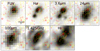 |
Fig. A.1. Similar to Fig. 1, but CO J = 2-1 emission and 1.3 mm continuum superimposed on the GALEX FUV (Gil de Paz et al. 2007), Hα (Gil de Paz et al. 2003), Spitzer IRAC1 at 3.6 μm (Brown et al. 2014), Spitzer MIPS 24 μm (Brown et al. 2014), Herschel MIPS at 100μm (Fisher et al. 2014), and VLA L-band at 1.425 GHz (Hunt et al. 2005) continuum maps, as well as the H I gas intensity map (Lelli et al. 2012). The CO emission coincides with emissions at FUV, Hα, and radio continuum, which trace star formation, along with stellar emission at 3.6 μm. Meanwhile, the hot and cold dust emission at 24 μm and 100 μm show a slight offset (∼3″) from the CO emission. The extended emission at 1.3 mm generally covers the emission at all bands shown here, except for H I gas. Emission at the 1.3 mm continuum falls between the two peaks of H I gas emission, and CO emission is also shifted from one of the H I peaks by ∼2″. A clear offset is shown between H I gas and CO gas and the 1.3 mm continuum. An offset between CO gas and H I gas has also been observed in another metal-poor galaxy, Sextans B (Shi et al. 2016). |
All Tables
All Figures
|
Fig. 1. CO J = 2–1 emission and 1.3 mm continuum superimposed on the HST V-band image from Izotov & Thuan (2004, PropID: 9400). The red contours denote the CO J = 2–1 integrated line intensity at the resolution of 1 |
| In the text | |
|
Fig. 2. CO J = 2–1 spectra from the merged, obs-17 and obs-19 data cubes. The spectra are smoothed to a velocity resolution of 3 km s−1 and extracted from the area defined by the 3σ contour as shown in Fig. 1. The 1σ uncertainty is 0.72, 0.72, and 1.39 mJy, respectively. The grey dashed line denotes the marginal detection at ∼46 km s−1. |
| In the text | |
|
Fig. 3. SED of IZw18, with CIGALE best fit adopting a delayed star formation history, a Draine & Li (2007) dust model, and a radio component. A modified blackbody fit is shown with a grey line. Photometric data are from Hunt et al. (2014), except for at 1.3 mm. The 3σ upper limit at 1.3 mm is shown as in the red star. The radio emission is also fitted with a cutoff model including a free-free component and a synchrotron component as introduced in Klein et al. (2018) (see more in the Sect. 4.1), which is indicated by the green curves. |
| In the text | |
|
Fig. 4. Infrared luminosity (top left) and SFR (derived from the emission at FUV and 24 μm, bottom left) versus |
| In the text | |
|
Fig. 5. LC II/LCO(1−0) ratio as a function of the metallicity (left) and specific SFR (right). IZw18 (red star) is compared to the galaxies compiled in Zanella et al. (2018, see references therein). The errorbar reflects the uncertainties of stellar mass and SFR. Pearson’s correlation coefficients for the regression fits are shown in each panel. |
| In the text | |
|
Fig. A.1. Similar to Fig. 1, but CO J = 2-1 emission and 1.3 mm continuum superimposed on the GALEX FUV (Gil de Paz et al. 2007), Hα (Gil de Paz et al. 2003), Spitzer IRAC1 at 3.6 μm (Brown et al. 2014), Spitzer MIPS 24 μm (Brown et al. 2014), Herschel MIPS at 100μm (Fisher et al. 2014), and VLA L-band at 1.425 GHz (Hunt et al. 2005) continuum maps, as well as the H I gas intensity map (Lelli et al. 2012). The CO emission coincides with emissions at FUV, Hα, and radio continuum, which trace star formation, along with stellar emission at 3.6 μm. Meanwhile, the hot and cold dust emission at 24 μm and 100 μm show a slight offset (∼3″) from the CO emission. The extended emission at 1.3 mm generally covers the emission at all bands shown here, except for H I gas. Emission at the 1.3 mm continuum falls between the two peaks of H I gas emission, and CO emission is also shifted from one of the H I peaks by ∼2″. A clear offset is shown between H I gas and CO gas and the 1.3 mm continuum. An offset between CO gas and H I gas has also been observed in another metal-poor galaxy, Sextans B (Shi et al. 2016). |
| In the text | |
Current usage metrics show cumulative count of Article Views (full-text article views including HTML views, PDF and ePub downloads, according to the available data) and Abstracts Views on Vision4Press platform.
Data correspond to usage on the plateform after 2015. The current usage metrics is available 48-96 hours after online publication and is updated daily on week days.
Initial download of the metrics may take a while.