| Issue |
A&A
Volume 652, August 2021
|
|
|---|---|---|
| Article Number | A112 | |
| Number of page(s) | 10 | |
| Section | Planets and planetary systems | |
| DOI | https://doi.org/10.1051/0004-6361/202141300 | |
| Published online | 19 August 2021 | |
Instability times in the HD 181433 exoplanetary system
1
Instituto de Astronomia, Geofísica e Ciências Atmosféricas, Universidade de São Paulo,
Brazil
e-mail: alves.raphael@usp.br
2
Instituto de Astronomía Teórica y Experimental, Observatório Astronómico, Universidad Nacional de Córdoba,
Argentina
3
Facultad de Ciencias Astronómicas y Geofísicas and Instituto de Astrofísica de La Plata, Universidad Nacional de La Plata,
Argentina
Received:
13
May
2021
Accepted:
21
June
2021
The present work consists of a study of the dynamical stability of a three-body system that takes advantage of the Shannon entropy approach to estimate the diffusivity (DS) in a Delaunay’s action-like phase space. We outline the main features of a numerical computation of DS from the solutions of the equations of motion and, thereupon, we consider how to estimate a macroscopic instability timescale, τinst, (roughly speaking, the lifetime of the system) associated with a given set of initial conditions. Through such estimates, we are able to characterize the system’s space of initial conditions in terms of its orbital stability by applying numerical integrations to the construction of dynamical maps. We compare these measures of chaotic diffusion with other indicators, first in a qualitative fashion and then more quantitatively, by means of long direct integrations. We address an analysis of a particular, near-resonant system, namely HD 181433, and we show that the entropy may provide a complementary analysis with regard to other dynamical indicators. This work is part of a series of studies devoted to presenting the Shannon entropy approach and its possibilities as a numerical tool providing information on chaotic diffusion and the dynamical stability of multidimensional dynamical systems.
Key words: celestial mechanics / planets and satellites: dynamical evolution and stability / chaos / diffusion / instabilities
© ESO 2021
1 Introduction
Stability is a basic concern when studying dynamical systems and the issue becomes more complicated (hence, tending to become less general) as it is shifted from near-integrable to non-integrable scenarios. Indeed, distinct definitions of stability are found in the literature, such as in the Hill and the Lagrange stability criteria (Barnes & Greenberg 2006), as recurrent examples in the context of celestial mechanics. In addition, it is known that chaos is a common dynamical feature of any system with more than one degree of freedom (Laskar 1989; Sussman & Wisdom 1992; Contopoulos 2002; Nesvornný & Ferraz-Mello 1997; Ferraz-Mello et al. 1998; Martí et al. 2016). The very essence of chaos consists of a strong sensibility with regard to the system’s initial parameters and initial conditions, which prevent us from reaching deterministic results. One of the main problems is how to approach such a property of the phase space in the sense of establishing any possible correlation between the onset of chaotic scenarios and the occurrence of noticeable dynamical phenomena (“events”) in the evolution of the system.
Studies on the dynamics of N-body systems usually consist of numerical integrations of the equations of motion, followed by the application of a numerical tool to explore the solutions, such as the frequency analysis (Laskar 1993; Laskar & Correia 2009), the spectral method (Michtchenko & Ferraz-Mello 2001; Alves et al. 2016), or any other known dynamical indicator of structure and chaoticity (Dvorak et al. 2004; Ramos et al. 2015; Martí et al. 2016). In Mel’nikov & Shevchenko (1998) and Popova & Shevchenko (2013), for example, a statistical approach was applied to separate regular from chaotic motion by integrating sets of initial parameters in two different timespans, T1 and T2 (T2 > T1), and then comparing the shifted peaks of the histograms for the logarithms of the maximum Lyapunov characteristic exponents (mLCEs, see Benettin et al. 1980) computed for the simulated trajectories in each time window. The shifting of the exponents to lower values is naturally expected for regular regimes of motion. Overall, we may notice that such studies are typically concerned with discriminating regular and quasi-periodic motion from chaotic ones and, thus, basically detach stable regimes from those where the motion through connected chaotic layers culminate in an exponential divergence of the nearby trajectories and, furthermost, possible dynamical instabilities.
Generally, the stability of multiple-body systems may be undoubtedly verified by long numerical simulations of their motion through time. Accordingly, it is possible to build up the so-called “lifetime-maps” by integrating the trajectories from grids of many initial conditions (ICs) (Tsiganis et al. 2005; Wittenmyer et al. 2012, 2013; Horner et al. 2019), where the system’s disruption times1 are obtained from the direct numerical solutions of the equations of motion. Such a scheme eventually proves too costly from a computational point of view: sometimes a single numerical integration spans up to times T elapsing ≳109 orbital periods of the innermost body.
An alternative procedure to determine the stability of a single solution consists of following the evolution of some proper action-like variable, I, and then modeling the time course of its variance, that is: var(I) versus time. Usually, for computing the variance, an ensemble of ICs in a small neighborhood around an initial point I0 should be considered (Martí et al. 2016). If the diffusion is normal, var(I) ~Dt, with the diffusion coefficient D (hereafter, also referred to as diffusivity) estimated as the constant rate at which the variance grows with time. Later on, the instability times may be estimated through D, assuming a constant rate for the growth of the variance as a function of time. The lifetime of the system may be approximated as ~ 1∕D (Martí et al. 2016).
In this sense, Giordano & Cincotta (2018) presented an interesting tool to investigate diffusion in multidimensional dynamical systems, based on the application of the Shannon entropy (see Shannon 1948). Therein they showed that the time evolution of the entropy S can be applied to compute a diffusivity DS, by assuming that, in chaotic configurations, the long-course of proper action-variables resembles a random-walk motion, andthe correlations between phase states are lost along time. They also showed that estimations of DS could still be derived even if the diffusion was not normal. A first application of such a technique in the context of celestial mechanics was presented by Beaugé & Cincotta (2019) in a study of the 2/1 mean motion resonance (MMR) of the elliptic restricted three-body problem (R3BP). In their study, it was found (for the first time) a good agreement between estimates of the instability times τinst (S) ~ 1∕DS and the disruption times tdis given by direct integrations.
In Cincotta et al. (2021a,b) the Shannon entropy approach was first applied to instability scenarios arising in the planetary 3BP, and the diffusivity, DS, was featured as a candidate for dynamical indicator. In such works, the analysis was addressed at distinct planetary architectures and also aimed at distinct goals. In Cincotta et al. (2021a), a compact system of Neptune-mass planets (HD 20003) was briefly presented and a single solution of its phase space was analyzed applying different numerical parametrizations, the derived τinst (S) being compared with long-term direct simulations. In Cincotta et al. (2021b), a global analysis of the phase space (a, e) (a – semi-major axis; e – eccentricity) of a system with giant-planets near the 7/1 MMR (HD 181433) was obtained through the construction of diffusion charts of a wide region of the outer planet’s phase plane. Such diffusion charts were, in fact, given in terms of the τinst (S)-estimates and, thus, they were called τinst-maps therein. Henceforth, we follow such a nomenclature.
In the present paper, we revisit the problem of the HD 181433 exoplanetary system, focusing on the outer planet’s phase space and with a particular interest in the dynamical features around its nominal solution (Horner et al. 2019). Let us recall that Horner et al. (2019) made use of lifetime maps to state that the current position of the system, as well as close-by ICs in the (a2, e2)-space, is stable up to 108 yr. Following Cincotta et al. (2021b), we develop a study comparing the instability times derived from a Shannon entropy approach against the direct integration of the equations of motion solved with an N-body simulator (hereafter called Ncorp). Such comparisons are done both for short-time simulations, where we tried to correlate the chaotic diffusion estimates with other dynamical indicators, and also for long-time simulations where we properly compared the system’s event times obtained via entropy estimation (Shannon) and direct integrations (Ncorp).
In contrast to what was presented in Cincotta et al. (2021b), which included a preliminary analysis of a wider range of ICs in the outer planet’s space, here we are concerned with the application of the Shannon entropy approach to the analysis of the phase space around the small vicinity of the system’s nominal position. First, we verify the competence of the diffusion estimates on identifying dynamical structures of stable and unstable motion, and then we check how such measures are in agreement with the results from Horner et al. (2019). Also, we take into consideration additional regions of the outermost planet’s semi-major axis to analyze how the estimates correlate with the dispersion obtained in the instability time distributions generated from direct simulations (see, e.g., Rice et al. 2018 and Hussain & Tamayo 2020); and then again if the diffusion estimates corroborate the chaotic structures obtained with other dynamical indicators.
Our work is an additional step on a course of studies dedicated to reporting on the usefulness of the Shannon entropy as a complementary technique in the dynamical analysis of planetary systems. The following section outlines the theoretical concepts adopted in our study, from the dynamical modeling of the problem to the basic theory of the Shannon entropy technique. Section 3 is devoted to the dynamical analysis and numerical experiments with HD 181433 exoplanetary system. Our summary and conclusions are given in Sect. 4.
2 Theoretical background
2.1 The (planar) Hamiltonian model
Here, we are concerned with Np-planetary systems, namely, systems formed by a central star of mass, m0, with Np ≥ 2 orbiting bodies (planets) of masses mi < m0 (1 ≤ i ≤ Np). We assume a coplanar configuration, such that the planetary motion has 2Np degrees of freedom and, hence, the system’s Hamiltonian set-up may be recast as a function of the (orbiting) bodies’ coordinates and momenta. To this end, we refer to the canonical set of variables  of the Jacobi formulation (Beaugé et al. 2007), and write the Hamiltonian of the system as
 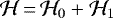 , with the Keplerian part given by
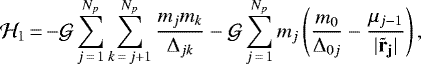
 (1)
(1)
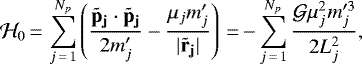
and the perturbation  written as:
 (2)
(2)
as showed in Beaugé et al. (2007). In the previous equations, the mass factors are defined as 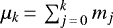 and the reduced masses are
  ; Δjk are the relative distances between the jth and kth bodies (Δ0j is the distance between the jth planet and the central star) and
  designates the universal gravitational constant. The last member in Eq. (1) may be written in terms of the classical Delaunay action variables:
  and
and  (ai and ei being the Jacobian osculating elements of the ith body). Such action variables are canonically conjugated to the angles (Mi, ωi) (namely, the mean anomalies and the arguments of the pericenters, respectively).
Via a recourse to the total angular momentum constraint,  (Ferraz-Mello et al. 2005), the number of degrees of freedom of the system may be reduced to 2Np − 1.
In our study, we numerically simulated the evolution of the 3BP in HD 181433, applying an N-body routine (Ncorp, see e.g. Cincotta et al. 2021a,b) that solves the equations of motion in the Jacobi reference frame. The code integrates in rectangular coordinates  , and later onthe respective values of the (osculating) orbital elements are recovered through classical coordinate transformations.
2.2 Shannon entropy theory applied to N-body solutions
Let us drop for a while the sub-index, i, identifying each individual planet in the system and its respective phase variable.
Applying the Shannon approach as in Cincotta et al. (2021b) we consider a pair of functions of the dynamical action variables, explicitly I ≡ L2 and J ≡ G2, being (L, G) the pair of Delaunay actions of the planar problem. In fact, our definitions essentially disregard the mass parameters, and namely we assume L2 = a and G2 = a(1 − e2), as proposed in Cincotta et al. (2021a).
Given an initial condition (IC), the equations of motion are numerically solved: the resulting evolutions of the semi-axis a and the eccentricity e are projected onto the (I, J)-plane, where a suitable partition is defined. The latter consists of q bi-dimensional disjoint cells covering a box of size [−ΔI, ΔI] × [−ΔJ, ΔJ], centered in the correspondent initial value (I0, J0). Then, q0 ≤ q cells are filled by the phase values (I(t), J(t)) during the integration process.
Regarding the sizes of the partition box, we followed Cincotta et al. (2021a,b) and defined the quantities ΔI and ΔJ based on a Hill-stability criteria (Marchal & Bozis 1982; Gladman 1993; Barnes & Greenberg 2006). We set a minimum distance Δmin given in terms of the mutual Hill’s radius RHill (Marzari & Weidenschilling 2002) of the orbits:
![\begin{equation*}\Delta_{\textrm{min}}\,{=}\,2\sqrt{3}R^{(i,j)}_{\textrm{Hill}}; \quad R^{(i,j)}_{\textrm{Hill}}\,{=}\, \left[\frac{(m_{i}+m_j)}{3m_0}\right]^{1/3}\frac{(a_{i}+a_j)}{2}.\end{equation*}](/articles/aa/full_html/2021/08/aa41300-21/aa41300-21-eq13.png) (3)
(3)
The criteria is always applied to adjacent bodies such that j = i + 1, i ≥ 1. In Marzari (2014), Δmin is assumed as an estimate of the “threshold value marking the transitions from stable to unstable orbits” (in timescales comparable to Gyr). In the present context, however, such criteria are used in a less rigorous sense.
We defined an interval Δa ≡ Δmin, taken in the semi-axis. In our formulation, Δmin is a fixed parameter applied to delimit the extents of a box of phase values in the plane (a, e), centered at the initial values (a0, e0). As for the eccentricities, the boundaries were set Δe = 0.5 (the singular cases e0 − Δe < 0 and e0 + Δe > 1 being avoided through internal conditions of the routine).
Afterwards, the respective values of Δa and Δe are used to obtain the partition box dimensions ΔI and ΔJ, within which the occupation probability of the kth cell, μk, and the number of occupied cells q0(t) are computed (Cincotta & Giordano 2018; Giordano & Cincotta 2018; Cincotta & Shevchenko 2020). Let us emphasize that the partition is constructed in all the Np phase planes (I, J) correspondent to each integrated trajectory.
It is also important to remark that each individual orbit is solved simultaneously with an ensemble of ne systems displaced inside a small range (δa, δe) in the near vicinity of the nominal initial values (a0, e0) of each body, giving rise to a set of shadow trajectories that will be accounted in the computation of an averaged value of S (Cincotta et al. 2021a,b).
The Shannon entropy  is calculated along the integration process and the time-averaged rate ⟨d S(t)∕dt⟩ is numerically computed ∀t ≥ t0, being t0 an adjustable “minimum time” at which the routine starts to estimate the derivative. Such an operation is done by means of a least square fit of the discrete data S(t). A diffusivity DS may be associated with the rate within which the pair (I, J) spreads through an area Σ(I, J) of the phase space, namely:
 (4)
(4)
as proposed in Cincotta et al. (2021a,b). In Eq. (4), we explicitly recall the fact that the diffusivity (hence, the instability time) is calculated for the ith planet and an individual instability time, τinst,i, can be estimated as
 (5)
(5)
where ΔIi and ΔJi are the half-lengths of the partition box centered at the respective initial values (I0,i, J0,i), 1 ≤ i≤ Np. The factor K is a dimensionless constant of the order of unity. Herein, we set K = 1, following Cincotta et al. (2021a,b).
Let us recall that Eq. (5) would lead to τinst →∞ as DS → 0, that is, when the system evolves on an invariant tori. Therein, the expected periodicity of the perturbations leads to bounded motions of slow diffusion. Since it makes no sense to speak of physical stability up to infinity times, an upper limit for the instability times ought to be predefined, which we address later in this text.
Finally, a global instability timescale for the planetary system may be obtained as the minimum value of the individual τinst,i,
 (6)
(6)
and, for a given set of ICs, Eq. (6) is associated with an expectation of the time within which instabilities manifest in large-scale and the destruction of the system is likely (Beaugé & Cincotta 2019; Cincotta et al. 2021a,b).
Further explanations can be found extensively in the literature (Giordano & Cincotta 2018; Cincotta et al. 2018; Cincotta & Shevchenko 2020; Beaugé & Cincotta 2019).
3 HD 181433 planetary system
3.1 Architecture of the nominal solution
HD 181433 is a three-planet system with a lighter innermost body (0.02 MJup, Bouchy et al. 2009) and two giant planets in wider orbits, all orbiting a K-type star of mass m0 = 0.86 M⊙. In the first architecture proposed by Bouchy et al. (2009), the authors informed an inherent unstable character of the system. New solutions were derived by Campanella (2011) and Horner et al. (2019), both relocating the system near resonant regions involving the outermost pair: a 5/2 MMR in Campanella (2011) and a 7/1 MMR in Horner et al. (2019). In the present work, we adopted the best-fit solution proposed by Horner et al. (2019), since it deals with data from the latest observational missions.
The latest architecture of such a system, with a small inner planet closer to the host star and two giant planets in wider orbits, may be approximated to a simpler model by neglecting the effects of the innermost body: numerical integrations (Cincotta et al. 2021b) have shown that the presence of the lighter body does not globally disturb the motion of the two external ones in long-term timescales. Hence, we have assumed a three-body model composed by the host star and the two outer bodies (planets c and d). Throughout this section, we use the subscripts 1 and 2 to refer to HD 181433c and HD 181433d, respectively.
Table 1 shows the orbital parameters and their respective uncertainties, for each planet: namely, we have the minimum masses (msini), the semi-major axes (a), the eccentricities (e), the inclination of the orbital planes (which we have fixed to 90 deg since the orbits are set coplanar), the orbital periods (P) and the argument of pericenter (ω). We applied the indicated values of T0 (the time of passage at the pericenter) to calculate the initial mean anomalies Mi (i = 1, 2).
Figure 1 displays results for a large integration of the nominal solution of Horner et al. (2019), hereafter referred to as IC (A0). The orbital parameters given in Table 1 were numerically integrated with the Ncorp routine, using a Runge-Kutta (R-K) integrator in a time-span T = 1 Gyr. The long-term stability of the solution is clear in the two upper plots, where the evolution of the semi-major axes and eccentricities are exposed.
A long-period variation of ~105 yr is noticed inboth middle panels, mainly in the right-hand one, where the time evolution of the outer planet’s eccentricity e2 is shown. The bottom-left plot shows, in blue, the time evolution of the secular angle Δϖ≡ ϖ1 − ϖ2 (ωi corresponds to ϖi for coplanar orbits), while the green dots correspond to the resonant angle2 θ1 = 6σ1. While no libration was observed for any resonant angle associated with the 7/1 MMR, the difference in longitudes of pericenter shows a large-amplitude oscillation (~125 deg) around 180 deg.
Finally, the lower right-hand panel shows the mLCE (ζ) as computed along the system’s evolution. We plotted log10ζ versus t (in logarithmic scale). The curve shows an asymptotic behavior for ζ which implies a chaotic solution. We checked that the mLCE reaches ζ ~ 10−4.6 yr−1 at the end of the integration, resulting TL ~ 105 yr.
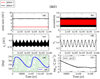 |
Fig. 1 Long-term evolution over 1 Gyr of the reduced two-planet system with initial orbital parameters equal to the nominal values (hereafter IC (A0)) given in Table 1. Top: evolution of (a) the semi-axes and (b) the ecccentricities. Middle: (c) shorter interval of a2 vs t; (d) e2 vs t. An oscilatory motion of period ~105 yr is evident. Bottom: (e) evolution of the secular angle Δϖ = ϖ1 − ϖ2 (blue) superposed on the evolution of the resonant angle θ1 = 6σ1 = 7λ2 − λ1 − 6ϖ1 (green); (f) evolution of the mLCE computations (ζ) for the solved trajectories. |
Orbital parameters of HD 181433c (planet 1) and HD 181433d (planet 2) as given by Horner et al. (2019), both orbiting a star of mass m0 = 0.86 M⊙.
3.2 Diffusivity DS as a stability indicator: τinst-maps in the near-vicinity of (A0)
In order to explore the surrounding domain of the nominal solution (A0), we focused on the dynamics of the outer planet. In Fig. 2, we present a set of six dynamical maps constructed in the pseudo action-action (a2, e2) and action-angle (a2, M2) planes of ICs, obtained through the numerical integration of a 100 × 100-mesh of ICs.
Panels a–d of Fig. 2 show the outcomes of pure integrations: in a and b, the equations of motion were solved concomitantly with the variational equations in T = 1 Myr, and the respective MEGNO values ⟨Y ⟩ of each solution were obtained through computations of the norm of the deviation vector of infinitesimally close trajectories (Cincotta & Simó 2000). In the frames c and d, we show the eccentricity-indicator (Dvorak et al. 2004): therein, we used the parameter A(e2) = e2,max −e2,min (Ramos et al. 2015; Charalambous et al. 2018), namely, the maximum amplitude reached by the outer planet’s eccentricity within 1 Myr.
We may enhance small variations on the chaotic levels by plotting the logarithm of the rescaled MEGNO, namely ⟨Y′ ⟩ = ⟨Y ⟩− 1.99, as it is presented in maps a and b. It is known that regular orbits have ⟨Y ⟩ ≤ 2 (Cincotta & Simó 2000): they are indicated by the darkest blue tones in the top frames. Values of ⟨Y ⟩ > 3 (i.e., log10⟨Y′⟩≳ 0) denote solutions of high chaotic levels (green, yellow, and red tones). Regions indicated with ⟨Y ⟩ between 2 and 3 (i.e. − 2 ≲ log10⟨Y′⟩≲ 0) exhibit mild chaotic motion. In all the integrations, the cut-off value was set to  .
.
As we can see in Fig. 1, solution (A0) (black dot in the maps) is mildly chaotic, lying outside the domain of the 7/1 MMR. Typical resonant structures (chain of resonant islands) are clear in the (a2, M2)-maps, with regular solutions around the centers marked with white “X”-symbols in M20 ~ 280 deg and M20 ~ 330 deg; note that (A0) lies quite near a hyperbolic solution (black “X”), thus explaining the high chaos that is seen in the range of a2 corresponding to the 7/1 MMR in Fig. 2a.
The maps e and f in Fig. 2 present two τinst-maps, constructed from the same mesh of 100 × 100 ICs: using Eq. (6), these charts are parametrized by the instability timescales, τinst(S), estimated for each simulated trajectory. At this time, each node of the mesh represents an IC evaluated through integrations of ne + 1 planetary pairs, that is, the “real” condition plus ne shadow trajectories. In a way that is different from results (a–d), the computations in the Shannon approach were spanned to 105 yr (one tenth of the time-span used before). Here, we used ne = 5.
We already mentioned how Eq. (5) may be shown to be problematic as we approach slow diffusion in phase space (with DS → 0). Our numerical precision of 10−13 induced us to set a computational uppermost limit of τinst ~ 1014 yr to the trajectories corresponding to such a case of very low diffusivity. Since any computation is undoubtedly affected by loss of precision due to many types of uncertainties, we decided to use, in a first analysis, a maximum range of 1012.5 yr (~ 3 × 10¹² yr) as a new uppermost value of τinst-estimates, at which we could still obtain a good resolution at the diffusion levels.
Although it lies in a chaotic zone, the maps e and f reveal that (A0) is characterized by long-term stability (i.e., slow diffusion), with a τinst(S) > 109 yr. Even the highly chaotic zones (e2 ~ 0.5) display diffusion rates that imply instability times greater than 100 Myr, a result that corroborates the study of Horner et al. (2019) in which they found a broad region of stability of orders > 100 Myr, surrounding the nominal position of the system, while the unstable regions appeared further from (A0), for ICs with a20 ≲ 6.3 AU. The correspondence between the resonant structures detailed by the instability levels in panels e and f (e.g., the resonance width, the islands of the 7/1 MMR, the separatrices) and by the chaotic layers seen in panels a and b indicates a certain correlation between structure, chaoticity and instability times.
Our results indicate that the space of ICs in (a2, e2) and (a2, M2) surrounding the solution of (A0) is characterized by a broad region of chaotic, albeit bounded motion. Regular motion, at least within 1 Myr, is only expected in the near-vicinity of the elliptic points indicated in the (a2, M2)-maps, where typical resonant structures were found.
In the next section, we focus our study on specific regions of HD 181433 phase space, aiming for a more quantitative comparison of our results. We selected three ICs by simply changing the initial value of a2 (the remaining orbital elements fixed to the corresponding values given in Table 1). Defining ICs (A1), (A2), and (A3) with the respective initial values for the outer semi-axis being a20 (A1) = 5.75 AU, a20 (A2) = 4.62 AU and a20 (A3) = 5.50 AU, we wanted, in a certain way, to observe responses from different regimes of motion, mostly when compared to (A0). In Cincotta et al. (2021b), one may verify that (A1) lies in between the 11/2 MMR and the 6/1 MMR; (A2) is over the outermost boundary of the 4/1 MMR; and (A3) is near but not too close to the 5/1 MMR. Additionally, Fig. 8 gives an indication of the positions of such ICs within the a2 -subspace.
 |
Fig. 2 Dynamical maps for the HD 181433 system, constructed over the (a2, e2) (top) and (a2, M2) (bottom) planes of ICs and obtained from the numerical solutions of a mesh of 100 × 100 ICs. The grid sizes are 0.004 AU in a2, 0.0005 in e2 and 1 deg inM2. (a–b) MEGNO-maps showing the rescaled value ⟨Y′⟩ = ⟨Y ⟩− 1.99. (c–d) e2-maps of the maximum amplitude of variation of e2 within T = 1 Myr. (e–f) τinst-maps obtained from DS-estimates. The (a2, M2)-maps show the chain of resonant islands generated by the 7/1 MMR, inside which a stable motion is expected. In all the bottom panels, the “X”-symbols mark the elliptic (white) and hyperbolic (black) solutions. The black dot indicates (A0). In maps a through d, integrations were carried out to 1 Myr; in the case of e and f the time-span was set ten times lower. |
3.3 Local dispersion of nearby solutions: tdis against τinst
Rice et al. (2018) studied the dispersion of instability times (as determined through long-term N-body simulations) of nearby ICs in a toy model of equally spaced three-planetary systems. They found that the calculated values of instability times seem to follow a log-normal distribution covering up to two orders of magnitude. Hussain & Tamayo (2020) found similar results related to tightly-packed systems, showing that the standard deviations of the ITDs were surprisingly similar (about 0.5 orders of magnitude) for a wide range of system parameters and ICs. In the present section, we analyze whether HD 181433 also exhibits such a dispersion and whether the Shannon entropy approach is able to reproduce such characteristics.
It should be noticed that the very essence of a chaotic system is its unpredictability. Thus, there are neither deterministic results on hand nor specific ways to derive a precise instability time. Such a feature is illustrated in Fig. 3, where the disruption time distributions coming from direct integrations of ICs taken around a small vicinity of (A1) and (A3) are displayed. Both panels present the results of simulations performed with distinct integrators: in the case of (A1), we show the correlation between solutions obtained with a Bulirsch-Stoer (B-S) and a Runge-Kutta of 7/8th order (R-K) routine; for (A3), we exhibit the B-S results versus those obtained with an Everhart’s Radau15 integrator (Everhart 1985).
The top panel in Fig. 3 corresponds to a rectangular grid of ICs, equally distributed around an area with upper and lower limits displaced within an interval δ = 10−3 around (A1). Such displacements were both taken in a2 and e2, which means that we integrated a total of 1156 ICs uniformly distributed within the ranges [5.749, 5.751]AU × [0.468, 0.470]. Analogously, the bottom panel shows integrations for a grid of 39 × 39 ICs around (A3), taking the same displacement δ in a2 and e2. Both panelsreveal no evidences of any correlations between the results: they are rather distributed densely and randomly around what would be the (apparent) most probable disruption times, namely, ~ 107 yr for (A1) and ~106 yr for (A3). In both cases the observed dispersion around the apparent averages is generally the same, that is, approximately greater than an order of magnitude independently of the chosen integrator (we note that the distributions cover up to three orders of magnitude in time).
We then conducted an analogous experiment, comparing the direct integrations using the B-S integrator and the τinst-estimates obtained with the Shannon approach. We simulated a large set of ICs equally distributed around the nominal values of (A1), (A2), and (A3), within rectangular grids of sizes [−δ, δ] ≡ [−10−3, 10−3] in semi-axis a2 and eccentricity e2. We notice that such a value is approximately the minimum uncertainty interval given for the semi-major axes and eccentricities (see Table 1, also Horner et al. 2019). We also recall that in the Shannon approach, the ICs inside the mesh were again “subdivided” into (ne + 1) = 6 shadow trajectories composing an ensemble of solutions (the radius of such an ensemble was taken an order of magnitude lower than δ).
While the direct integrations were set to span large times (1 Gyr), with the respective disruption times tdis of each solution being identified, the Shannon estimates were computed within T = 0.1 Myr.
The corresponding correlation diagrams obtained for each solution are presented in the panels of Fig. 4. It is possible to see a good agreement between the data, which is more explicit in the case of (A1), where we notice that in spite of the dispersion being greater for the Shannon results, both approaches show a distribution with a heavier concentration of points at timescales of ~ 107 yr.
In the results for (A3), the largest dispersion is observed in the direct integrations, with some solutions reaching tdis > 108 yr. Nevertheless, most of the data points concentrates in the (approximate) ranges [3 × 10⁵, 2 × 10⁷] yr for tdis, and [4 × 10⁴, 2 × 10⁶] yr for τinst.
Otherwise, a different behavior is observed for (A2). Both sets of data show a high dispersion of results, being such a dispersion clearly more severe in the case of the Shannon estimates, where the distribution is bimodal. Overall, the data distribution is concentrated within timescales on the order of ~ 106 yr, in the ordinate axis, and ~107 yr in the abscissas. It is quite a curious behavior, and it has led to a deeper investigation of the local dynamics nearby (A2).
Before proceeding on an individual analysis of (A2), we may close our statistical overview with Table 2, which shows the principal weights calculated for the distributions obtained in the panels of Figs. 3 and 4; namely, Table 2 displays the averages (or expected values) μ and the standard deviations σ for each sample of tdis (applying different N-body integrators) and τinst-estimates. It should be remarked that such distributions were plotted in log-scaled diagrams and, thus, both μ and σ were obtained considering log-normal instability time distributions (Rice et al. 2018; Hussain & Tamayo 2020). In the cases of (A1) and (A3), it is clear that the averages given by Shannon estimates are underestimated in regard tothe direct integrations; for (A2), we observe the contrary (we note that the respective σ is also greater in this case). In any situation, however, the differences are at most of one order of magnitude.
In considering again the middle frame of Fig. 4, we ask what such a dispersion may indicate about the dynamics around (A2). With this question in mind, we constructed the dynamical maps in the (a2, e2) plane of ICs, as shown in Fig. 5. The MEGNO-map (left-hand) and the τinst-map (middle) were both built over a fine mesh (see caption) of ICs integrated for T = 105 yr. In the right-hand panel, the lifetime map of the same domain was obtained from long direct integrations of a 50 × 50-grid of ICs.
From the computations of ⟨Y ⟩, we notice the stochastic layer encompassing mild to strong chaos. Disruptive solutions within the integration time-span are shown in dark red tone. The nominal position of (A2), marked with a black dot, suggests that such IC is immersed in the separatrix-like domain of the 4/1 commensurability. Chaos seems to grow outwards the apparent center of the resonance (a2 ~ 0.46 AU), and also as e2 reaches higher values.
A long-term stable resonant core is highlighted in the τinst-map, in the middle, and also in the lifetime map at right. Nonetheless, there is no correlation between the existence of quasi-periodic solutions (log10(⟨Y ⟩− 1.99) ~−2) and long-term stability: pay attention that the inner long-lasting zone (where both τinst and tdis are greater than 108 yr) appears chaotic within 0.1 Myr in the left-hand panel.
The discrepancy seen in the middle diagram of Fig. 4 could be explained by the particular location of IC (A2), which is on the edge of a region immersed in a widespread chaos, which results in the destruction of the system within times ≲ 10 Myr, but also close to ICs of long-term stability (≳100 Myr). This is easily verified through the direct simulations in the right-hand map of Fig. 5.
The τinst-estimates are compared against the pure numerical integrations of the right-hand frame in a more explicit fashion through the diagram of Fig. 6, where we present the respective correlation of (τinst, tdis) for an equal set of ICs, integrated in a 50 × 50-mesh. In the diagram, as well as in the maps, the transition of dynamical regimes, which seems to characterize the close-by domain of (A2), is clear.
In the maps of Fig. 5, we see (A2) lying near long-term solutions, in which the direct simulations (right-hand panel) showed no strong instabilities within times that are comparable to the integration time-span (tdis ~ 0.1–1 Gyr). Then there are solutions in which the disruptions occurred around half million years and tens of million years; and, finally, we may see for higher eccentricities, the onset of a destructive chaos, where pure integrations elapsed over no longer than ~ 0.1 Myr. Such a phase transition appears smoother in the chart of disruption times compared to the τinst-map, where we notice anoverestimation of the domain of long-lasting ICs. Such an overestimation appears in the border of the separatrix for the whole e2 -subspace of ICs.
An intricate dynamics shall be expected in the border of resonant domains: therein the perturbations arising from Eq. (2) yield a stochastic layer in the vicinity of the separatrix. On the other hand, the existence of a strong nearby MMR (in general, a low-order one) can contribute for maintaining regions of long-term stability, and for which we see a correlation through the τinst-map, as suggested by the central portion of both middle and right-hand maps of Fig. 5. Such a configuration, where long stability is close to stochastic areas, might not be well modeled as a Brownian-type motion, but by anomalous diffusive transport instead, which is characteristic of phenomena such as stickiness (Tsiganis et al. 2000).
At the same time, as we go to higher values of eccentricities and outward the resonance center, an overlap with neighbouring high-order resonances is expected (Chirikov 1979). The stochastic layers of adjacent resonances merge allowing a large-scale diffusion of the actions along the connected network (Hadden & Lithwick 2018; Petit et al. 2020). As the space is fully covered by overlapping resonances, the trajectories are well approximated by a random walk (normal diffusion). In the maps of Fig. 5, this may be extrapolated to values where a20 < 4.5 AU and a20 > 4.7 AU.
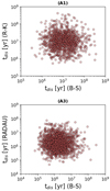 |
Fig. 3 Top: correlation diagram between the disruption times tdis obtained from direct integrations of ICs in the close neighborhood of (A1), applying a Bulirsch-Stoer (B-S) and a Runge-Kutta (R-K) integrator. Bottom: analogous result for (A3), but comparing B-S and Radau15 integrators. The same numerical precision was set for all the simulations. |
Expected values μ and standard deviations σ obtained for the distributions of tdis and τinst (see text), all of them computed admitting a log-normal distribution of instability/disruption times (see, e.g., Rice et al. 2018; Hussain & Tamayo 2020).
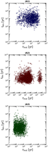 |
Fig. 4 Correlation diagrams between the estimated instability times τinst and the numerical disruption times tdis, obtained for sets of ICs integrated around the initial values (a20, e20): 1225 ICs surrounding (A1) (top), 2500 around (A2) (middle) and 1600 in the case of (A3) (bottom). |
 |
Fig. 5 Dynamical maps constructed over the (a2, e2) space of ICs of HD 181433. Left-hand and middle panels: a 100 × 100-mesh of ICs was integrated in T = 0.1 Myr, with grid sizes being 0.004 AU in a2 and 0.001 in e2. Right-handpanel: disruption times obtained from N-body simulation spanned to 1 Gyr, over a grid of 50 × 50 ICs. The black dot indicates the nominal position of (A2) in each plane. |
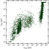 |
Fig. 6 Correlation diagrams between the estimated instability times τinst(S) and the numerical disruption times tdis, obtained for the same 50 × 50-mesh of ICs.The results from the Shannon approach were simulated within 0.1 Myr, while the direct simulations spanned 1 Gyr. The red dot highlights the expected values (τinst, tdis) for the nominal position of (A2), as given in Table 2. |
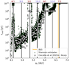 |
Fig. 7 Distribution of the respective values of τinst-estimates for a set of 104 ICs in the range 4.5AU ≤ a2 ≤ 7.0AU. Straight black lines highlight the exact positions of the lowest-order MMRs identifiable, and the yellow one indicates the nominal position of the real system (near the 7/1 MMR). The white squares represent the disruption times tdis as obtained by Cincotta et al. (2021b) from direct integrations of 374 ICs on almost the same segment (there, the grid size in a2 was ~ 6.5 × 10⁻³ AU). |
3.4 Instability times in the extended a2-subspace
We extended our approach to wider regions of HD 181433’s phase space, waiving our previous local analysis in favor of a macroscopic and more global study. We had a particular interest in verifying the response of the Shannon entropy method when applied to regions corresponding to other resonances. Thus, we took a set of 104 ICs inside the interval 4.5AU ≤ a2 ≤ 7.0AU, which leads to increments of 2.5 × 10⁻⁴ AU in a2. The remaining orbital elements were fixed to their nominal values (Table 1). The simulations were spanned to T = 105 yr, with the entropy, S, the diffusivity, DS, and the instability time, τinst, being evaluated for each ensemble of trajectories.
The outcomes from the simulations are depicted in Fig. 7, where the distribution of dark triangles displays the τinst-estimates of the respective solutions. In this particular analysis, we set 1010 yr as the cut-off value for lowest diffusive trajectories. As a matter of fact, the approximate age of HD 181433 star is ≈ 6.7 Gyr (Trevisan et al. 2011); thus, a rough comparison between τinst(S) and the actual system age can be made.
The straight black lines signalize the exact position of some MMRs found in such a domain. The respective ratios n1 ∕n2 are identified at the top of the frame (ni being the ith mean motion). The yellow line gives the position of the (A0) (at left of the 7/1 MMR). We marked with white squares the disruption times obtained in Cincotta et al. (2021b) through direct integrations of 374 ICs taken within the same interval of a2.
There is a correlation between peaks of stability and the nominal positions of some commensurabilities, mainly for the ratios k∕1 (k > 1 being an integer), but also present in the case of the 11/2 MMR. Both the time distributions (τinst and tdis) show reasonable agreement in this aspect, evincing that such resonances are characterized by slower diffusion of the action variables (consequently, longer lasting solutions) with respect to the external neighborhood. Indeed, it is known that MMRs can be responsible for protecting the global integrity of planetary systems on long timescales by avoiding close encounters and likely crossings of the trajectories whenever the system is found near equilibria domains (elliptic points), even in highly eccentric scenarios.
In the panels of Fig. 8, an amplification of the previous collection of 104 estimates isshown, in three distinct sections of the considered interval of a2. In addition to the tdis-distribution of Cincotta et al. (2021b), we plotted a second distribution of disruption times, obtained using a R-K integrator simulating a finer mesh of ICs (grid size of ~2.5 × 10⁻³ AU in a2) and marked therein with red dots. The colored lines in each panel also indicate the location of the single ICs (A1), (A2), and (A3), explored in the previous section. The same logic of colors used in Fig. 4 is followed here.
The panels of Fig. 8 unveil an agreement between predictions and pure integrations that is overall satisfactory. Even though some discrepancies are seen, we remark that on many occasions the computations done with the Shannon approach elapsed overup to four orders of magnitude less in terms of the time of integration than the pure simulations, and a reasonable accordance could still be recovered. The notorious exceptions can be noticed in the separatrix structures that mark the main resonances in the considered domain.
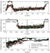 |
Fig. 8 Three sections of the instability time distributions obtained from the solutions over a segment of ICs in a2, previously presented in Fig. 7. We have added new direct integrations performed with a R-K integrator, plotted here with red markers. The thin colored lines in each panel highlight the nominal position of the individual ICs (A1) in blue, (A2) in red, and (A3) in green, following the color code applied in Fig. 4. |
4 Discussion
In the present paper, we analyze the characteristics of the architecture of the HD 181433 exoplanetary system, applying known dynamical indicators and then we focused on the macroscopic stability aspects of such a system. The equations of motion of the 3BP were numerically solved in the Jacobi-frame formulation, using specific dynamical indicators to characterize the space of ICs of the orbital elements. At this stage, we introduced our own indicator, namely the τinst-estimates.
We find that the current configuration of HD 181433 system, proposed by Horner et al. (2019), is long-term stable and our long numerical simulation revealed a local chaoticity that dominates a small vicinity of the nominal solution. We verified that such a local chaos is due to the proximity to the separatrix of the 7/1 MMR. Furthermore, we checked that the nominal solution exhibits a slow diffusion, resulting in an instability timescale that would be larger than the age of the host-star (~ 7 Gyr, Trevisan et al. 2011).
Dynamical maps constructed with pure integrations and Shannon-evaluations showed the system lying near resonant structures generated by the 7/1 MMR, but outside the libration domain. A long simulation revealed that any possible combination of a resonant argument circulates, while the Δϖ angle oscillates around 180 deg in periods of ~105 yr. Overall, the system’s behavior is ruled by this long-term stable periodic regime of motion.
By extending our analysis to wider regions of the outer semi-major axis, we observe that some high-order commesurabilities are associated with long-term stability, which means that the respective solutions displayed slow diffusion of the actions in the Shannon approach.
Taking into consideration the limitation demonstrated by the method when applied to a rather complex region, such as the separatrix of the 4/1 MMR, where non-ergodic phenomena such as stickiness may lead the system to depart from normal and move to anomalous diffusion processes (Tsiganis et al. 2000), we find an agreement between tdis and τinst-estimates for an extensive ensemble of ICs of distinct regions of the phase space, as presented in Figs. 4 and 7. In addition, it is interesting to notice that the correlation between the stochastic structures (identified with the MEGNO) and the diffusion levels (from τinst-estimates), as verified through Fig. 2, is not recovered in the domains presented in the maps of Fig. 5, another piece of evidence in support of possible stickiness affecting the solutions.
As has already been demonstrated in recent studies (Cincotta & Shevchenko 2020; Beaugé & Cincotta 2019; Cincotta et al. 2021a,b), the hypothesis of nearly ergodicity is a major prerogative in a Shannon entropy approach, but may not be suitable in the case of the separatrix. More studies shall address this concern.
Here, we demonstrate that the application of the Shannon entropy in planetary systems yields credible estimations of the instability times and may therefore be used to give relevant dynamical information that complements those derived from other dynamical indicators.
Even though the use of ensembles increases the computational costs with respect to a single simulation, it is still about three orders of magnitude faster than the raw integration of a single IC for the age of the system. Moreover, since the diffusion rate may be estimated for each planet of the system, it is also possible to determine which body plays a key role in the chaotic diffusion process and how the system is disrupted. A more detailed examination of this feature will be explored in future works.
Acknowledgements
This work was supported by grants from Coordenação de Aperfeiçoamento de Pessoal de Nível Superior (CAPES) and the Universidade de São Paulo from Brasil; the CONICET, the Universidad Nacional de La Plata and the Universidad Nacional de Córdoba from Argentina. The authors thank the Brazilian section of the PLATO mission team and the grants from FAPESP (2016/13750-6) and CNPq (303540/2020-6). We also thank Elielson Soares Pereira, with whom some fruitful discussions were exchanged in the beginning of this work, as well as the anonymous referee and the language editor for their useful comments and corrections that helped us to improve the manuscript.
References
- Alves, A. J., Michtchenko, T. A., & Tadeu dos Santos, M. 2016, CeMDA, 124, 311 [NASA ADS] [CrossRef] [Google Scholar]
- Beaugé, C., & Cincotta, C. M. 2019, CeMDA, 131, 52 [CrossRef] [Google Scholar]
- Barnes, R., & Greenberg, R. 2006, ApJ, 647, L163 [CrossRef] [Google Scholar]
- Beaugé, C., Ferraz-Mello, S., & Michtchenko, T. A. 2007, Planetary Masses and Orbital Parameters from Radial Velocity Measurements, Extrasolar Planets, ed. R. Dvorak (Hoboken: Wiley) [Google Scholar]
- Benettin, G., Galgani, L., Giorgilli, A., et al. 1980, Meccanica 15, 9 [NASA ADS] [CrossRef] [Google Scholar]
- Bouchy, F., Mayor, M., Lovis, C., et al. 2009, A&A, 496, 527 [NASA ADS] [CrossRef] [EDP Sciences] [Google Scholar]
- Campanella, G. 2011, MNRAS, 418, 1028 [NASA ADS] [CrossRef] [Google Scholar]
- Charalambous, C., Martí, J. G., Beaugé, C. et al. 2018, MNRAS, 477, 1414 [CrossRef] [Google Scholar]
- Chirikov, B. V. 1979, Phys. Rep., 52, 263 [NASA ADS] [CrossRef] [Google Scholar]
- Cincotta, P. M., & Giordano, C. M. 2018, CeMDA, 130, 74 [NASA ADS] [CrossRef] [Google Scholar]
- Cincotta, P. M., & Simó, C. 2000, A&AS, 147, 205 [NASA ADS] [CrossRef] [EDP Sciences] [Google Scholar]
- Cincotta, P. M., & Shevchenko, I. I. 2020, Physica D, 402, 132235 [CrossRef] [Google Scholar]
- Cincotta, P. M., Giordano, C. M., Martí, J. G., & Beaugé, C. 2018, CeMDA, 130, 7 [NASA ADS] [CrossRef] [Google Scholar]
- Cincotta, P. M., Giordano, C. M., Alves Silva, R. et al. 2021a, CeMDA, 133, 7 [NASA ADS] [CrossRef] [Google Scholar]
- Cincotta, P. M., Giordano, C. M., Alves Silva, R. et al. 2021b, Physica D, 417, 32816 [Google Scholar]
- Contopoulos, G. 2002, Order and Chaos in Dynamical Astronomy (Berlin, Heidelberg: Springer-Verlag) [CrossRef] [Google Scholar]
- Dvorak, R., Pilat-Lohinger, E., Schwarz, R. et al. 2004, A&A, 426, L37 [NASA ADS] [CrossRef] [EDP Sciences] [Google Scholar]
- Everhart, E. 1985, IAU Coloq., 83, 185 [NASA ADS] [Google Scholar]
- Ferraz-Mello, S., Nesvornný, D., & Michtchenko, T. A. 1998, ASP Conf. Ser., 149, 81 [Google Scholar]
- Ferraz-Mello, S., Michtchenko, T. A., Beaugé, C., et al. 2005, Extrasolar Planetary Systems, eds. R., Dvorak, F., Freistetter, & J., Kurths (Berlin: Springer), 683 [Google Scholar]
- Giordano, C. M., & Cincotta, P. M. 2018, CeMDA, 130, 35 [NASA ADS] [CrossRef] [Google Scholar]
- Gladman, B. 1993, Icarus, 106, 247 [Google Scholar]
- Hadden, S., & Lithwick, Y. 2018, ApJ, 156, 95 [CrossRef] [Google Scholar]
- Horner, J., Érdi B., Wittenmyer, R. A., Wright, D. J. et al. 2019, AJ, 158, 100 [NASA ADS] [CrossRef] [Google Scholar]
- Hussain, N., & Tamayo, D. 2020, MNRAS, 491, 5258 [CrossRef] [Google Scholar]
- Laskar, J. 1989, Nature, 338, 237 [NASA ADS] [CrossRef] [Google Scholar]
- Laskar, J. 1993, Physica D, 67, 115 [Google Scholar]
- Laskar, J., & Correia, A. C. M. 2009, A&A, 496, L5 [NASA ADS] [CrossRef] [EDP Sciences] [Google Scholar]
- Marchal, C., & Bozis, G. 1982, CMDA, 26, 311 [Google Scholar]
- Martí, J. G., Cincotta, P. M., & Beaugé, C. 2016, MNRAS, 460, 1094. [NASA ADS] [CrossRef] [Google Scholar]
- Marzari, F. 2014, MNRAS, 442, 1110. [NASA ADS] [CrossRef] [Google Scholar]
- Marzari, F., & Weidenschilling, S. J. 2002, Icarus, 156, 570 [Google Scholar]
- Mel’nikov, A. V., & Shevchenko, I. I. 1998, Sol. Syst. Res., 32, 480 [Google Scholar]
- Michtchenko, T., & Ferraz-Mello, S. 2000, Icarus, 149, 357 [Google Scholar]
- Michtchenko, T., & Ferraz-Mello, S. 2001, AJ, 122, 474 [NASA ADS] [CrossRef] [Google Scholar]
- Nesvornný, D., & Ferraz-Mello, S. 1997, A&A, 320, 672 [Google Scholar]
- Petit, A., Pichierri, G., Davies, M. B. et al. 2020, A&A, 641, A176 [NASA ADS] [CrossRef] [EDP Sciences] [Google Scholar]
- Popova, E. A.,& Shevchenko, I. I. 2013, ApJ, 769, 152 [NASA ADS] [CrossRef] [Google Scholar]
- Ramos, X. S., Correa-Otto, J. A., Beaugé, C. 2015, CeMDA, 123, 453 [NASA ADS] [CrossRef] [Google Scholar]
- Rice, D. R., Rasio, F. A., & Steffen, J. H. 2018, MNRAS, 481, 2205 [CrossRef] [Google Scholar]
- Shannon, C. 1948, Bell Syst. Tech. J., 27, 379 [Google Scholar]
- Sussman, G. J., & Wisdom, J. 1992, Science, 257, 56 [NASA ADS] [CrossRef] [PubMed] [Google Scholar]
- Trevisan, M., Barbuy, B., Eriksson, K., et al. 2011, A&A, 535, A42 [NASA ADS] [CrossRef] [EDP Sciences] [Google Scholar]
- Tsiganis, K., Varvoglis, V., & Hadjidemetriou, J. D. 2000, Icarus, 146, 240 [NASA ADS] [CrossRef] [Google Scholar]
- Tsiganis, K., Varvoglis, V., & Dvorak, R. 2005, CeMDA, 92, 71 [NASA ADS] [CrossRef] [Google Scholar]
- Wittenmyer, R. A., Horner, J., Tuomi, M. et al. 2012, ApJ, 753, 169 [NASA ADS] [CrossRef] [Google Scholar]
- Wittenmyer, R. A., Horner, J., & Marshall, J. P. 2013, MNRAS, 431, 2150 [NASA ADS] [CrossRef] [Google Scholar]
Any resonant argument θi of a ni ∕nj = (k1 + k2)∕k1 (planar) MMR may be written as a linear combination of two independent critical angles, σ1 and σ2, with
σ1 = (1 + r)λ2 − rλ1 − ϖ1,
σ2 = (1 + r)λ2 − rλ1 − ϖ2,
being r = k1 ∕k2 the ratio between the integers that define the nominal resonance (k2 designates the order of the resonance) (Michtchenko & Ferraz-Mello 2000). In the case of a commensurability of order k2 = 6, such as the 7/1 MMR, it is expected the following harmonics: θ1 = 6σ1, θ2 = 6σ2, θ3 = 3σ1 + 3σ2, θ4 = 4σ1 + 2σ2, θ5 = 2σ1 + 4σ2, θ6 = 5σ1 + σ2 and θ7 = σ1 + 5σ2.
All Tables
Orbital parameters of HD 181433c (planet 1) and HD 181433d (planet 2) as given by Horner et al. (2019), both orbiting a star of mass m0 = 0.86 M⊙.
Expected values μ and standard deviations σ obtained for the distributions of tdis and τinst (see text), all of them computed admitting a log-normal distribution of instability/disruption times (see, e.g., Rice et al. 2018; Hussain & Tamayo 2020).
All Figures
|
Fig. 1 Long-term evolution over 1 Gyr of the reduced two-planet system with initial orbital parameters equal to the nominal values (hereafter IC (A0)) given in Table 1. Top: evolution of (a) the semi-axes and (b) the ecccentricities. Middle: (c) shorter interval of a2 vs t; (d) e2 vs t. An oscilatory motion of period ~105 yr is evident. Bottom: (e) evolution of the secular angle Δϖ = ϖ1 − ϖ2 (blue) superposed on the evolution of the resonant angle θ1 = 6σ1 = 7λ2 − λ1 − 6ϖ1 (green); (f) evolution of the mLCE computations (ζ) for the solved trajectories. |
| In the text | |
|
Fig. 2 Dynamical maps for the HD 181433 system, constructed over the (a2, e2) (top) and (a2, M2) (bottom) planes of ICs and obtained from the numerical solutions of a mesh of 100 × 100 ICs. The grid sizes are 0.004 AU in a2, 0.0005 in e2 and 1 deg inM2. (a–b) MEGNO-maps showing the rescaled value ⟨Y′⟩ = ⟨Y ⟩− 1.99. (c–d) e2-maps of the maximum amplitude of variation of e2 within T = 1 Myr. (e–f) τinst-maps obtained from DS-estimates. The (a2, M2)-maps show the chain of resonant islands generated by the 7/1 MMR, inside which a stable motion is expected. In all the bottom panels, the “X”-symbols mark the elliptic (white) and hyperbolic (black) solutions. The black dot indicates (A0). In maps a through d, integrations were carried out to 1 Myr; in the case of e and f the time-span was set ten times lower. |
| In the text | |
|
Fig. 3 Top: correlation diagram between the disruption times tdis obtained from direct integrations of ICs in the close neighborhood of (A1), applying a Bulirsch-Stoer (B-S) and a Runge-Kutta (R-K) integrator. Bottom: analogous result for (A3), but comparing B-S and Radau15 integrators. The same numerical precision was set for all the simulations. |
| In the text | |
|
Fig. 4 Correlation diagrams between the estimated instability times τinst and the numerical disruption times tdis, obtained for sets of ICs integrated around the initial values (a20, e20): 1225 ICs surrounding (A1) (top), 2500 around (A2) (middle) and 1600 in the case of (A3) (bottom). |
| In the text | |
|
Fig. 5 Dynamical maps constructed over the (a2, e2) space of ICs of HD 181433. Left-hand and middle panels: a 100 × 100-mesh of ICs was integrated in T = 0.1 Myr, with grid sizes being 0.004 AU in a2 and 0.001 in e2. Right-handpanel: disruption times obtained from N-body simulation spanned to 1 Gyr, over a grid of 50 × 50 ICs. The black dot indicates the nominal position of (A2) in each plane. |
| In the text | |
|
Fig. 6 Correlation diagrams between the estimated instability times τinst(S) and the numerical disruption times tdis, obtained for the same 50 × 50-mesh of ICs.The results from the Shannon approach were simulated within 0.1 Myr, while the direct simulations spanned 1 Gyr. The red dot highlights the expected values (τinst, tdis) for the nominal position of (A2), as given in Table 2. |
| In the text | |
|
Fig. 7 Distribution of the respective values of τinst-estimates for a set of 104 ICs in the range 4.5AU ≤ a2 ≤ 7.0AU. Straight black lines highlight the exact positions of the lowest-order MMRs identifiable, and the yellow one indicates the nominal position of the real system (near the 7/1 MMR). The white squares represent the disruption times tdis as obtained by Cincotta et al. (2021b) from direct integrations of 374 ICs on almost the same segment (there, the grid size in a2 was ~ 6.5 × 10⁻³ AU). |
| In the text | |
|
Fig. 8 Three sections of the instability time distributions obtained from the solutions over a segment of ICs in a2, previously presented in Fig. 7. We have added new direct integrations performed with a R-K integrator, plotted here with red markers. The thin colored lines in each panel highlight the nominal position of the individual ICs (A1) in blue, (A2) in red, and (A3) in green, following the color code applied in Fig. 4. |
| In the text | |
Current usage metrics show cumulative count of Article Views (full-text article views including HTML views, PDF and ePub downloads, according to the available data) and Abstracts Views on Vision4Press platform.
Data correspond to usage on the plateform after 2015. The current usage metrics is available 48-96 hours after online publication and is updated daily on week days.
Initial download of the metrics may take a while.