| Issue |
A&A
Volume 652, August 2021
|
|
|---|---|---|
| Article Number | A145 | |
| Number of page(s) | 11 | |
| Section | Planets and planetary systems | |
| DOI | https://doi.org/10.1051/0004-6361/202140923 | |
| Published online | 25 August 2021 | |
KMT-2018-BLG-1743: planetary microlensing event occurring on two source stars
1
Department of Physics, Chungbuk National University,
Cheongju
28644,
Republic of Korea
e-mail: cheongho@astroph.chungbuk.ac.kr
2
University of Canterbury, Department of Physics and Astronomy,
Private Bag 4800,
Christchurch
8020, New Zealand
3
Korea Astronomy and Space Science Institute,
Daejon
34055, Republic of Korea
4
Korea University of Science and Technology,
217 Gajeong-ro,
Yuseong-gu,
Daejeon
34113, Republic of Korea
5
Max Planck Institute for Astronomy,
Königstuhl 17,
69117
Heidelberg, Germany
6
Department of Astronomy, The Ohio State University,
140 W. 18th Ave.,
Columbus,
OH
43210, USA
7
Department of Particle Physics and Astrophysics, Weizmann Institute of Science,
Rehovot
76100, Israel
8
Center for Astrophysics | Harvard & Smithsonian 60 Garden St.,
Cambridge,
MA
02138, USA
9
Department of Astronomy, Tsinghua University,
Beijing
100084,
PR China
10
School of Space Research, Kyung Hee University,
Yongin,
Kyeonggi
17104, Republic of Korea
Received:
30
March
2021
Accepted:
30
June
2021
Aims. We present the analysis of the microlensing event KMT-2018-BLG-1743. The analysis was conducted as a part of the project, in which previous lensing events detected in and before the 2019 season by the KMTNet survey were reinvestigated with the aim of finding solutions of anomalous events with no suggested plausible models.
Methods. The light curve of the event, with a peak magnification Apeak ~ 800, exhibits two anomaly features, one around the peak and the other on the falling side of the light curve. An interpretation with a binary lens and a single source (2L1S) cannot describe the anomalies. By conducting additional modeling that includes an extra lens (3L1S) or an extra source (2L2S) relative to a 2L1S interpretation, we find that 2L2S interpretations with a planetary lens system and a binary source best explain the observed light curve with Δχ2 ~ 188 and ~91 over the 2L1S and 3L1S solutions, respectively. Assuming that these Δχ2 values are adequate for distinguishing the models, the event is the fourth 2L2S event and the second 2L2S planetary event. The 2L2S interpretations are subject to a degeneracy, resulting in two solutions with s > 1.0 (wide solution) and s < 1.0 (close solution).
Results. The masses of the lens components and the distance to the lens are (Mhost/M⊙,Mplanet/MJ,DL/kpc)~(0.19−0.111+0.27,0.25−0.14+0.34,6.48−1.03+0.94) and ~(0.42−0.25+0.34,1.61−0.97+1.30,6.04−1.27+0.93) according to the wide and close solutions, respectively. The source is a binary composed of an early G dwarf and a mid M dwarf. The values of the relative lens-source proper motion expected from the two degenerate solutions, μwide ~ 2.3 mas yr−1 and μclose ~ 4.1 mas yr−1, are substantially different, and thus the degeneracy can be broken by resolving the lens and source from future high-resolution imaging observations.
Key words: gravitational lensing: micro / planets and satellites: detection
© ESO 2021
1 Introduction
The standard light curve of a two-object (lens and source) lensing event with a single lens and a single source (1L1S) has a smooth and symmetric form (Paczyński 1986). Under the approximation of a rectilinear relative lens-source motion, the lensing light curve of a 1L1S event is described by three lensing parameters of (t0, u0, tE) as
![\begin{equation*} A\,{=}\,{u^2+2 \over u \sqrt{u^2+4}};\qquad u\,{=}\, \left[ u_0^2 + \left({t-t_0 \over t_{\textrm{E}}} \right){}^2\right]^{1/2},\end{equation*}](/articles/aa/full_html/2021/08/aa40923-21/aa40923-21-eq3.png) (1)
(1)
where the individual lensing parameters represent the time of the closest lens-source approach, the lens-source separation (normalized to the angular Einstein radius θE) at t0, and the event time scale, respectively.
For a fraction of lensing events, light curves exhibit deviations from the 1L1S form. Such deviations are most commonly caused by the duality of the lens (Mao & Paczyński 1991) or the source (Griest & Hu 1993). Hereafter, we refer to the three-object events with binary lens or binary source stars as 2L1S or 1L2S events, respectively. At the time when such anomalous events were first found, for example, MACHO LMC 1 (Dominik & Hirshfeld 1994) and OGLE 7 (Udalski et al. 1994) 2L1S events and MACHO LMC 96-2 (Becker et al. 1997) 1L2S event, interpreting the observed lensing light curves was a challenging task due to the difficulty of modeling caused by various technical issues. The first of these issues was the increased number of lensing parameters with the addition of the extra lens or source component, and this made it difficult to find a lensing solution, that is, a set of lensing parameters that best explain the observed light curves, via a grid approach. Second, the χ2 surface in the parameter plane was complex, especially for 2L1S events, due to the discontinuity in lensing magnifications caused by the formation of caustics, and this made it difficult to find a solution via a simple χ2 minimization approach. Third, computing finite-source magnifications during the source star’s crossing over the caustic required heavy computations, and this hampered prompt interpretations of anomalous lensing events. The majority of these difficulties in the interpretation of multiple-object lensing events has been resolved with the adoption of sophisticated logic that is optimized for finding lensing solutions in a complex parameter space, such as the Markov chain Monte Carlo (MCMC) method, together with the development of efficient methods for computing finite-source magnifications, such as the map-making method, for example, Dong et al. (2009), the adaptive ray-shooting method, for example, Bennett et al. (2010), and the image contour method, for example, Gould & Gaucherel (1997) and Bozza et al. (2018). As a result, three-object modelings are routinely being conducted for most anomalous events.
For a minor fraction of anomalous events, it is known that the observed light curves cannot be explained by either a 2L1S or a 1L2S model. The difficulty of finding lensing solutions for these events suggests that interpreting their light curves requires more complex models than those including three objects. For some of these events, solutions including more than three objects were identified. Currently, there exist 14 confirmed cases of lensing events with models including more than three objects. See the list of these events in Table 1 of Han et al. (2021a). However, there still exist events for which no plausible model has been proposed.
In this paper, we present the analysis of the planetary lensing event KMT-2018-BLG-1743. The event was reinvestigated in the project of reanalyzing anomalous events, for which lensing light curves could not be explained by either a 2L1S or a 1L2S model, among the previous lensing events detected in and before the 2019 season by the Korea Microlensing Telescope Network (KMTNet: Kim et al. 2016). This project has led to the discoveries of the 3L1S events OGLE-2018-BLG-1700 (Han et al. 2020b) and OGLE-2019-BLG-0304 (Han et al. 2021c), in which the lenses have three components (planets in binary systems), the 2L2S event KMT-2019-BLG-0797 (Han et al. 2021a), in which both the lens and source are binaries, and the 3L2S event KMT-2019-BLG-1715 (Han et al. 2021b), in which the lens have three components and the source is composed of two stars. Here the notation “3L” indicates that the lens is a triple system. The event KMT-2018-BLG-1743 was known to be anomalous, but no detailed analysis has been presented due to the difficulty of explaining the anomalies with a three-object model. In this work, we check the feasibility of interpreting the KMT-2018-BLG-1743 light curve with the introduction of an extra lens or source component.
For the presentation of the work, we organize the paper as follows. In Sect. 2, we describe the observations of the lensing event and the data used in the analysis. In Sect. 3, we model the lensing light curve under various interpretations and present the results of these models. We specify the source type and estimate the angular Einstein radius of the event in Sect. 4. We determine the physical parameters of the lens system in Sect. 5, and discuss the degeneracy in the interpretation of the event in Sect. 6. We summarize the result of the analysis and conclude in Sect. 7.
2 Observations and data
The source star of the lensing event KMT-2018-BLG-1743 is located toward the Galactic bulge field. The equatorial and galactic coordinates of the source are  and (l, b) = (5°.694, −4°.792), respectively.The baseline magnitude of the source before the lensing magnification was Ibase = 19.81 according tothe KMTNet scale. We note that the source lies at a very dense field, toward which stellar images are, in most cases, heavily blended, and thus there exists, in general, little information about the stars of the field in public databases such as SIMBAD1. The magnification of the source flux induced by lensing was found from the post-season investigation of the 2018 season KMTNet data using the AlertFinder System (Kim et al. 2018).
The KMTNet group has conducted a microlensing survey since 2015 by utilizing three identical KMTNet telescopes. These telescopes are globally distributed in three continents of the Southern Hemisphere for the continuous coverage of lensing events: Australia (KMTA), Chile (KMTC), and South Africa (KMTS). Each telescope, with a 1.6 m aperture, is equipped with a camera providing a 2° × 2° field of view. The lensing event was located in the KMTNet BLG31 field, toward which observations were conducted with a 2.5 h cadence. Most images were acquired in the I band, and about one tenth of images were obtained in the V band. The I-band data were used for the light curve analysis, and the V -band data were used for the measurement of the source color.
Reduction of the data was conducted using the pySIS code developed by Albrow et al. (2009). The photometry code is a customized version of the difference imaging method (Tomaney & Crotts 1996; Alard & Lupton 1998), that was developed for the optimal photometry of stars located in a very dense star field. Additional photometry using the pyDIA software (Albrow 2017) was done for a subset of KMTC I- and V -band data to measure the color of the source and to construct the color-magnitude diagram (CMD) of stars around the source. We will describe the detailed procedure of the source color measurement in Sect. 4. Following the routine of Yee et al. (2012), the error bars of the data used in the analysis were readjusted by ![$\sigma\,{=}\,[\sigma_{\textrm{min}}^2+ (k\sigma_0){}^2]^{1/2}$](/articles/aa/full_html/2021/08/aa40923-21/aa40923-21-eq5.png) , where σ0 denotes the error bar estimated by the automated pipeline, and (σmin, k) represent the scatter of data and the rescaling factor used to make χ2 per degree of freedom become unity, respectively. In Table 1, we present the data rescaling coefficients along with the time range and the number of data points, Ndata, for the individual data sets.
, where σ0 denotes the error bar estimated by the automated pipeline, and (σmin, k) represent the scatter of data and the rescaling factor used to make χ2 per degree of freedom become unity, respectively. In Table 1, we present the data rescaling coefficients along with the time range and the number of data points, Ndata, for the individual data sets.
Figure 1 shows the lensing light curve of KMT-2018-BLG-1743. Inspection of the light curve reveals three characteristics. First, the light curve exhibits an anomaly in the falling side of the light curve. The anomaly is centered at HJD′≡HJD − 2 450 000 ~ 8258 (2018-05-19), and lasted for about 6 days. Second, the event was highly magnified. A 1L1S modeling conducted with the exclusion of the data around the anomaly in the wing yields (t0, u0, tE, ρ) ~ (8249.150, 5 × 10⁻⁶, 28.18 days, 2.46 × 10⁻³). Here ρ denotes the normalized source radius, which is defined by the ratio of the angular source radius, θ*, to the angular Einstein radius, θE, that is, ρ = θ*∕θE, and it is included in the modeling to account for possible finite-source effects that may occur when the lens passes over the surface of the source. In computing finite magnifications, we consider limb-darkening effects by adopting a linear coefficient of u = 0.5 from Claret (2000), considering that the source is an early G-type dwarf. The detailed procedure of the source type specificationis described in Sect. 4. The 1L1S model curve (dotted curve) is drawn over the data points in Fig. 1. The magnification at the peak of the light curve estimated from the 1L1S model is Apeak ~ 800. Third, the light curve exhibits an additional anomaly in the peak region as well as the anomaly in the wing. To better show this central deviation, we present the zoom-in view of the peak region in the inset of Fig. 1. The central deviation is most evident for the two KMTS data points taken at the epochs of HJD′ = 8249.430 and 8249.568, which exhibit deviations of ΔI = 0.45 mag and 0.21 mag from the 1L1S model, respectively. These deviations are much greater than the photometric uncertainties of nearby data points.
We checked the possibility of systematics in the data and the variability of the source or blend by inspecting the residual from the best-fit model that will be described in the following section. The residual is shown in Fig. 2. The top panel, with a time range of 8165 ≤HJD′≤ 8420 (225 days), and the middle panel, with 8305 ≤HJD′≤ 8323 (18 days), are presented to check long- and short-term systematics or variability in the data. The bottom panel, showing the residual in the time range of 8245 ≤HJD′≤ 8270 (25 day), during which the source was substantially magnified, is shown to check the possible systematics that might arise in the measurement of the light variation. It is found that the data in all inspected time ranges do not show any symptom of systematics or source variation.
An event with a very high magnification is an important target for follow-up observations due to the high chance of detecting planet-induced perturbations in the peak region of the light curve (Griest & Safizadeh 1998). Despite the very high magnification, no followup observation was conducted for KMT-2018-BLG-1743, because the KMTNet real-time AlertFinder (Kim et al. 2018) only began operation on 21 June 2018, that is, 40 days after the peak. Moreover, the AlertFinder was not applied to field BLG31 until 2019.
Data and error rescaling factors.
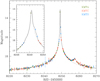 |
Fig. 1 Light curve of the microlensing event KMT-2018-BLG-1743. The inset shows the zoom-in view of the peak region. The two curves drawn over the data points are the model curves of the 1L1S (dotted) and the wide 2L2S (solid) solutions. The colors of the telescopes in the legend are chosen to match those of the data points in the light curve. |
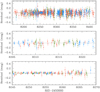 |
Fig. 2 Residual from the best-fit model (wide 2L2S model) in various time ranges. The top and middle panels show the residuals in the time ranges of 8165 ≤ HJD′≤ 8420 (225 days) and 8305 ≤HJD′≤ 8323 (18 days), respectively. The bottom panel shows the residual in the time range of 8245 ≤ HJD′≤ 8270 (25 day), during which the source was substantially magnified. |
3 Interpretation of the anomaly
A key for the interpretation of the event is to explain both anomalies, that is, the one in the peak and the other in the wing of the observed light curve. Hereafter, we refer to the individual anomalies as the central and peripheral anomalies, respectively. For the interpretation of the anomalies, we test various lensing models under 2L1S, 3L1S, and 2L2S interpretations. The 2L1S model is tested because a binary lens with a very low-mass companion can generate two short-term anomaly features in the lensing light curve under a certain lens system configuration. As already mentioned and to be fully discussed in Sect. 3.1, it is difficult to precisely describe the observed data with a 2L1S model. The 3L1S and 2L2S models are tested to check whether the anomaly features can be described by introducing an additional lens or source component. In the following subsections, we describe the procedures of the individual modelings and present the results of the analyses.
3.1 2L1S interpretation
In principle, a 2L1S lensing light curve can produce two anomaly features. This is possible because a binary lens with a very small mass ratio between the lens components, M1 and M2 < M1, such as a binary pair composed of a planet and a host, induces two sets of caustics, in which one is located close to M1 (central caustic) and the other is located away from M1 (planetary caustic). Then, two anomaly features can arise when a source passes both the central and planetary caustics.
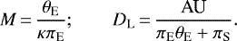
Keeping this possibility in mind, we conducted a 2L1S modeling of the light curve. In addition to the 1L1S parameters, a 2L1S modeling requires one to include additional parameters to describe the lens binarity. These parameters are (s, q, α), which denote the projected M1 –M2 separation (normalized to θE), the mass ratio q = M1∕M2, and the angle between the source trajectory and the M1 –M2 axis (source trajectory angle). The modeling was carried out in two steps. In the first step, we conducted grid searches for s and q with multiple starting points of α evenly distributed in the range of 0 < α ≤ 2π. In this procedure, the lensing parameters (t0, u0, tE) were searched for using a downhill approach based on the MCMC method. Besides these parameters, a lensing modeling requires one to include two flux parameters (fs,i, fb,i) for each observatory, and these parameters are obtained from the regression of the observed flux, Fi, to the model by Fi (t) = fs,iA(t) + fb,i. We constructed a Δχ2 map in the s–q plane from the modeling, and identified local solutions in the Δχ2 map. Figure 3 shows the Δχ2 map in the log s– logq plane obtained in this procedure. In the second step, we conducted an additional modeling to refine the individual local solutions found in thefirst step by allowing all parameters to vary. This two-step procedure allows us to identify degenerate solutions, it they exist.
The modeling yielded a predicted solution: a source passing both the central and planetary caustics produced by a planetary lens system.The lensing parameters of the best-fit 2L1S model are listed in Table 2 along with the χ2 value of the fit. We note that the binary parameters are represented as (s2, q2) to distinguish them from the parameters of a possible third lens mass, (s3, q3), to be discussed in the following subsection. The estimated binary parameters are (s2, q2) ~ (1.16, 9 × 10⁻⁵), which wouldindicate that the event was produced by a planetary system containing a planet with a very low planet-to-host mass ratio and a projected separation slightly larger than the Einstein ring of the host. The lens system configuration, showing the source trajectory with respect to the positions of the lens components and the resulting caustics, is shown in the upper panel of Fig. 4. The configuration shows that the central caustic is located very close to the host (M1), and the planetary caustic is located at a positionwith a separation s − 1∕s ~ 0.3 from M1 on the planet (M2) side with respect to the host. As expected, the source passes both the central and planetary caustics, and this produces the central and peripheral anomalies, respectively. We note that two anomaly features can also be produced by a close planet with a separation less than θE, that is, s < 1.0. This local solution appears in the Δχ2 map presented in Fig. 3. In this case, the induced planetary caustics have a different shape and number from those of the caustic induced by a wide planet with s > 1.0 (Han 2006).We found that the solution with a source trajectory connecting the planetary caustic induced by a planet with s < 1.0 and the central caustic results in a substantially worse fit, by Δχ2 = 340.5, than the presented solution with s > 1.0.
It is found that the 2L1S model is not adequate for the precise description of the data, and its fit to the data is worse than the fit of the model to be discussed in Sect. 3.3 by Δχ2 ~ 188. To demonstratethis inadequacy, in the left and right panels of Fig. 5, we present the 2L1S model curve and the residuals from the model in the central and peripheral anomaly regions, respectively. From the comparison of the data and the model in the central anomaly region, it is found that the two KMTS data points at HJD′ = 8249.430 and 8249.568 still exhibit considerable deviations from the model. It is also found that an important fraction of data points in the peripheral anomaly region lie outside the error bars from the model. The inadequacy of the model in describing the observed data suggests that a different interpretation of the event is needed.
We additionally check whether the deviations from the static 2L1S model can be explained by higher-order effects, especially the orbital motion of the lens. We check the higher-order effects because there have been two cases, in which an extra lens body was incorrectly inferred due to the omission of the lens orbital motion in the 2L1S modeling together with the sparse coverage of the grid parameter (s, q, α) space: MACHO-97-BLG-41 (Bennett et al. 1999; Albrow et al. 2000; Jung et al. 2013) and OGLE-2013-BLG-0723 (Udalski et al. 2015; Han et al. 2016). This check was done in two steps. In the first step, we explore the grid parameter space with an increased density by doubling the resolution of the grid in each dimension. It is found that this does not yield any local solution other than the solution presented in Table 2. In the second step,we consider the lens-orbital and microlens-parallax effects so that the source trajectory can be non-rectilinear. Considering these higher-order effects requires one to include four additional parameters: πE,N, πE,E, d s∕dt, and d α∕dt. The first two parameters represent the north and east components of the microlens-parallax vector πE, respectively,and the other two parameters indicate the change rates of the binary separation and the source trajectory angle, respectively. The model with the higher-order effects improves the fit by Δ χ2 = 51.4 with respect to the static model, but the fit is worse than the best model (in Sect. 3.3) by Δ χ2 = 136.8, still leaving significant deviations in the central anomaly region. Furthermore, the resulting value of the microlens parallax πE ~ 1.25 is absurdly high, yielding a primary lens mass of M1 ~ 0.02 M⊙, which is very unusual considering the very usual event time scale of tE ~ 31 days. All these facts indicate that the residual from the 2L1S model is not ascribed to high-order effects, and the unusual higher-order parameters are induced by the incorrect basis static model.
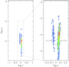 |
Fig. 3 Δχ2 map in the logs– logq parameter plane obtained from the 2L1S modeling. Points marked in different colors represent the regions with Δχ2 ≤ n(12) (red), Δχ2 ≤ n(22) (yellow), Δχ2 ≤ n(32) (green), Δχ2 ≤ n(42) (cyan), and Δχ2 ≤ n(52) (blue), where n = 5. The left panel shows the map in the region with − 1.0 < logs ≤ 1.0 and − 5.8 < logq ≤ 0.0, and the right panel shows the map in the narrower region with − 0.26 < logs ≤ 0.26 and − 5.6 < logq ≤−1.9. |
Lensing parameters of the 2L1S and 3L1S models.
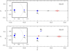 |
Fig. 4 Lens system configurations of the 2L1S (upper panel) and 3L1S (lower panel) models. In each panel, the inset shows the broad region including the positions of the lens components: blue dots marked by (M1, M2) for the 2L1S model and (M1, M2, M3) for the 3L1S model. The dotted circle in each inset represents the Einstein ring. The source motion is represented by a line with an arrow. The red closed figures represent the caustics. |
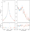 |
Fig. 5 Model curve of the 2L1S solution and the residuals from the model in the central (left panels) and peripheral (right panels) anomaly regions. |
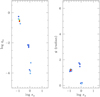 |
Fig. 6 Δ χ2 maps in the logs3– logq3 (left panel) and log s3–ψ (right panel) planes obtained from the 3L1S grid search. The color coding is same as that in Fig. 3, except that n = 1. |
3.2 3L1S interpretation
Not being able to find a 2L1S solution that precisely describes the observed light curve, we additionally examined a 3L1S model. We tested this model because the major deviation from the 2L1S model appeared in the central magnification region. If the lens has a third mass, M3, the central caustic induced by M3 may affect the magnification pattern of the central region (Gaudi et al. 1998; Han 2005), and this may explain the deviation from the 2L1S model in the central anomaly. A modeling considering a third lens component requires one to include additional parameters of (s3, q3, ψ), which represent the separation and mass ratio between M1 and M3, that is, q3 = M3∕M1, and the orientation angle of M3 as measured from the M1 –M2 axis with its origin at M1, respectively.
The 3L1S modeling was carried out in four steps. In the first step, we conducted a 2L1S modeling of the light curve with the exclusion of the data in each of the central and peripheral anomalies. This yielded three sets of 2L1Ssolutions, in which one was obtained with the exclusion of the data around the central anomaly (8248.0 ≤HJD′≤ 8250.0), and the other two solutions were obtained with the exclusion of the data around the peripheral anomaly (8252.0 ≤HJD′≤ 8270.0). In the second step, we conducted a 3L1S modeling, in which the parameters (s3, q3, ψ) were searched for using a grid approach, and the other parameters were searched for using a downhill approach. In this step, we fix the parameters related to M2, that is, (s2, q2, α), as the values of the solutions found from the 2L1S modeling conducted in the first step. In the third step, we refined the solutions found from the second step by releasing all parameters as free parameters. In the final step, we repeated the second and third steps for thethree sets of the 2L1S solutions found in the first step. It was found that the 3L1S solution starting from the M2 parameters obtained with the exclusion of the data around the central anomaly yielded the best-fit solution. Figure 6 shows the Δχ2 maps in the log s3– logq3 and log s3–ψ planes obtained from the grid modeling in the second step. The solutions resulting from the 2L1S solutions with the exclusion of the peripheral anomalies were worse than the best-fit model by Δχ2 ≳ 90.
Figure 7 shows the model curve and residuals from the best-fit 3L1S model in the central and peripheral anomaly regions. The lensing parameters of the solution are listed in Table 2 together with the χ2 value of thefit. It is found that the parameters of the 3L1S model related to the M1 –M2 pair are similar to those of the 2L1S model, and the parameters related to the additional lens component M3 are (s3, q3, ψ) ~ (0.12, 0.51, 65°). In the lowerpanel of Fig. 4, we present the lens system configuration for the 3L1S solution. The configuration is similar to that of the 2L1S solution, except that the extra lens component M3 induces a tiny astroid-shape caustic around M1. The source passes through the central caustic induced by M3, and this substantially reduces the 2L1S residuals, especially in the central anomaly region. The comparison of the fit with that of the 2L1S model, presented in Fig. 5, indicates that the 3L1S model provides a better fit than the 2L1S solution, by Δχ2 = 97.4. Although the fit of the 3L1S model looks fairly good, we reserve judgment the model until we test an additional interpretation in the following subsection.
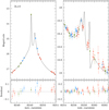 |
Fig. 7 Model curve of the 3L1S solution and the residuals from the model. Notations are same as those in Fig. 5. |
3.3 2L2S interpretation
We additionally checked the possibility that both the lens and source were binaries. We examined this model because 2L2S and 3L1S models occasionally yield similar light curves, as demonstrated in the cases of the lensing events KMT-2019-BLG-1953 (Han et al. 2020a) and KMT-2019-BLG-0797 (Han et al. 2021a). A modeling with the inclusion of an extra source star, S2, requires one to include additional parameters. These parameters are (t0,2, u0,2, ρ2, qF), which represent the time and separation of S2 at the closest approach to a reference position of the lens, the normalized radius of S2, and the flux ratio between the source stars, respectively. We use the notations of the lensing parameters related to the first source, S1, as (t0,1, u0,1, ρ1) to distinguish them from the parameters related to the second source. We started the 2L2S modeling with the three solutions obtained from the 2L1S modeling with the exclusion of the data around each of the central and peripheral anomalies. We then set the initial values of the parameters (t0,2, u0,2, ρ2, qF) considering the time and magnitude of the anomaly that was excluded in the initial 2L1S modeling.
The 2L2S modeling yielded two solutions that well described the data in both the central and peripheral anomalies. In Table 3, we list the lensing parameters and χ2 values of the fits for the two 2L2S solutions. It is found that one solution has a binary lens separation greater than unity (s ~ 1.05), and the other solution has a separation less than unity (s ~ 0.88). We refer to the solutions with s > 1.0 and s < 1.0 as “wide” and “close” solutions, respectively. The estimated mass ratio between the lens components is qwide ~ 1.2 × 10⁻³ for the wide solution and qclose ~ 3.7 × 10⁻³ for the close solution, and thus the mass of the companion is in the planetary-mass regime regardless of the solutions. We note that the binary separations of the pair of the degenerate solutions are not in the relation of sclose ~ 1∕swide, and the source trajectory angles of the two solutions, αwide ~ 47° and αclose ~ 73°, are substantially different from each other. This indicates that the degeneracy between the two solutions is not caused by the well-known close–wide degeneracy arising due to the similarity between the central caustics of the close and wide binaries with s and s−1 (Griest & Safizadeh 1998; Dominik 1999). Rather, it is caused by the lack of observations during the time interval 8248.6 ≲HJD′≲ 8249.6, when the wide and close solutions have single-peak and double-peak morphologies, respectively. For both solutions, the secondary source is fainter than the primary source with an I-band flux ratio of qF ~ 7%.
Figure 8 shows the lens system configurations of the two 2L2S solutions. The trajectories of the primary and secondary source stars are marked by S1 and S2, respectively.In each configuration, the tips of the arrows on the source trajectories represent the positions of S1 and S2 at a same epoch, and thus the configuration indicates that S2 trails S1 for both the wide and close solutions. Regardless of the solution, both the primary and secondary source stars cross the caustic, and the caustic crossings of S1 and S2 explain the central and peripheral anomalies, respectively. The model curves and the residuals from the models of the wide and close solutions in the regions of the anomalies are shown in Figs. 9 and 10, respectively. Despite the significant difference in the lens system configurations, it is found that both solutions result in similar fits to the data.
We find that the models obtained under the 2L2S interpretation provide substantially better fits to the observed data than the other models based on the 2L1S and 3L1S interpretations. This can be seen in the middle panel of Fig. 11, where we plot the cumulative distributions of the χ2 difference relative to the 2L1S model,that is, 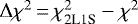 , for the 3L1Sand 2L2S (wide and close) models. We find that the fit of the wide (close) 2L2S model is better than the 3L1S and 2L1S models by Δχ2 = 90.8 (86.0) and 188.2 (184.3), respectively. As expected, the fit improvement occurs mainly in the anomaly regions. The comparison of the fits between the two 2L2S solutions indicates that the wide solution slightly better describes the observed data in the peripheral anomaly region than does the close solution, but the χ2 difference is small, Δχ2 = 4.8, and thus we consider the close model as a viable solution. The bottom panel show the contribution to the 2L2S fit improvement, that is,
  , by the individual data sets. It shows that the contribution to
  in the region around the central anomaly comes mostly from the KMTS data set, because the region is mainly covered by this data set, and the contribution in the peripheral anomaly region comes from both the KMTC and KMTS data sets. The fit improvement by both data sets further supports the validity of the model. On the other hand, the contribution to
  by the KMTA data set is small due to its spare coverage of both anomaly regions.
With the superiority of the fit to the data over the other models, we conclude that KMT-2018-BLG-1743 is a planetary microlensing event occurring on two source stars. A microlensing event with a binary lens and a binary source is very rare, and there were only three confirmed cases before the report of a new one in this work. The previously known 2L2S events include MOA-2010-BLG-117 (Bennett et al. 2018), OGLE-2016-BLG-1003 (Jung et al. 2017), and KMT-2019-BLG-0797 (Han et al. 2021a), among which MOA-2010-BLG-117L is a planetary system and the lenses of the other events are binaries with roughly equal masses. Then, KMT-2018-BLG-1743 is the fourth 2L2S event, and the second case with a lens identified as a planetary system.
We checked the feasibility of measuring the microlens parallax πE and the angular Einstein radius θE, which are the two observables needed to determine the physical lens parameters of the mass M and distance DL by
 (2)
(2)
Here κ = 4G∕(c2AU) and πS = AU∕DS represents the parallax of the source located at a distance DS (Gould 2000). For the πE determination, it is required to measure the deviation of the lensing light curve from a rectilinear form caused by the orbital motion of Earth around the Sun (Gould 1992). From the additional modeling considering the microlens-parallax effect, we found that it was difficult to securely determine πE, because the event time scale (tE ~ 28 days) was not long enough, and the photometric precision was not high enough to firmly detect subtle deviations induced by this second-order effect. Constraining the source orbital motion is even more difficult because the contribution of the flux from S2 is confined in the small region around the peripheral anomaly. For the estimation of θE, it is required to measure the normalized source radius ρ, which is determined from the deviation in the caustic-crossing parts of the lensing light curve caused by finite-source effects. With the measured ρ, the angular Einstein radius was determined by
 (3)
(3)
For both the close and wide 2L2S solutions, it was found that the normalized radius of the primary source, ρ1, was measured, although the normalized radius of the secondary source, ρ2, could not be securely measured. We note that, although ρ2 is not measured, the angular Einstein radius can be determined by θE = θ*,1∕ρ1 with the measurement of the angular stellar radius of S1, θ*,1. We will describe the detailed procedure ofdetermining the θ*,1 and θE in the following section.
Lensing parameters of the 2L2S model.
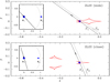 |
Fig. 8 Lens system configurations of the wide (upper panel) and close (lower panel) 2L2S models. Notations are same as those in Fig. 4, except that there are two source trajectories for the primary (S1) and the secondary (S2) source stars. The offset between the arrows on the two source-star trajectories indicates the relative position of the two sources. |
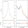 |
Fig. 9 Model curve of the wide 2L2S solution and the residuals from the model. Notations are same as those in Fig. 5. |
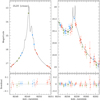 |
Fig. 10 Model curve of the close 2L2S solution and the residuals from the model. Notations are same as those in Fig. 4. |
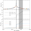 |
Fig. 11 Cumulative distributions of Δχ2 from the 2L1S model for the 3L1S and 2L2S (wide and close) models. The shaded area indicate the central (left) and peripheral (right) anomaly regions. |
4 Source stars and angular Einstein radius
We estimated the angular Einstein radius using the relation in Eq. (3) with the angular radius of the source estimated from its color and brightness. To estimate the reddening and extinction corrected (de-reddened) source color and brightness,  , we used the method of Yoo et al. (2004), in which the centroid of the red giant clump (RGC) in the CMD is used as a reference for calibration.
Figure 12 shows the locations of S1 and S2 with respect to the RGC centroid (red dot) in the instrumental CMD of neighboring stars around the source constructed using the pyDIA photometry of the KMTC I- and V -band data. The pair of the filled blue and green dots denote the positions of S1 and S2 based on the wide 2L2S solution, and the pair of the empty dots indicate the positions based on the close 2L2S solution. It shows that the locations of S1 estimated from the two solutions are nearly identical, and the locations of S2 are consistent within the uncertainty. We also present the Hubble Space Telescope (HST) CMD (Holtzman et al. 1998, brown dots)to show the source locations in the main-sequence branch. In order to determine the locations of S1 and S2, we first estimated the combined flux from the source stars,  , by conducting a 2L2S modeling including the I- and V -band pyDIA reduction of the data, and then estimated the flux values of the individual source stars by
 (4)
(4)
Here the subscript “p” denotes the passband of the observation, and  represents the flux ratio between the binary source stars measured in each passband. In Table 4, we list the measured instrumental colors and magnitudes of the RGC centroid,
  , the primary source,
  , and the secondary source,
  , together with the flux ratios measured in the I and V bands, qF,I and qF,V, respectively. We note that qF,I values presented in Table 4, which are derived from the pyDIA reduction, and Table 3, which is derived from the pySIS reduction, are slightly different due to the use of the data from different reductions.
With the measured instrumental values, we calibrated the color and brightness of each source using the offsets in color and magnitude from the RGC centroid, Δ(V − I, I), by
 (5)
(5)
where  are the de-reddened color and magnitude of the RGC centroid known from Bensby et al. (2013) and Nataf et al. (2013), respectively.This relation assumes that the source follows the same distribution of RGC stars. Under this assumption, the source and RGC centroid experience similar reddening and extinction, but we note that the granularity of the extinction may cause deviation from this approximation. We list the de-reddened colors and magnitudes of S1 and S2 in Table 4. The measured colors and magnitudes indicate that the primary source is an early G-type dwarf, and the secondary source is a mid M-type dwarf.
We then estimated the angular radius of the primary source, θ*,1, based on the measured de-reddened color and magnitude. We did not estimate the radius of the secondary source not only because its normalized radius ρ2 was not measured but also because the uncertainty of the measured color was very big2. The angular source radius was estimated from the (V − K)–θ* relation of Kervella et al. (2004), where V − K color was interpolated from V − I using the color–color relation of Bessell & Brett (1988)3. With the measured source radius, the angular Einstein radius and the relative lens-source proper motion were determined by θE = θ*,1∕ρ1 and μ = θE∕tE, respectively. In Table 5, we list the (θ*,1, θE, μ) values estimated from the wide and close solutions. The uncertainties of θ* and subsequent values of θE and μ are estimated not only based on the uncertainty of the measured source color, but also by adding ~ 7% error in quadrature to account for the scatter of RGC stars in the CMD caused by varying distance as well as the uncertainty arising in the (V − K)–θ* process. We note that the estimated angular Einstein radius of the wide solution, θE,wide ~ 0.18 mas, is substantially smaller than that of the close solution, θE,close ~ 0.31 mas, because the measured normalized source radius, ρwide ~ 2.1 × 10⁻³, is bigger than that of the close solution, ρclose ~ 1.2 × 10⁻³.
Source color and magnitude.
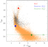 |
Fig. 12 Locations of the primary (S1) and secondary (S2) source stars in the instrumental color-magnitude diagram (CMD). The pair of the filled blue and green dots denote the positions of S1 and S2 based on the wide 2L2S solution, and the pair of the empty dots indicate the positions based on the close 2L2S solution. The red filled dot denotes the centroid of red giant clump (RGC). The HST CMD (brown dots) is presented to show the source locations in the main-sequence branch. |
Angular source and Einstein radii and relative lens-source proper motion.
5 Physical lens parameters
Not being able to measure the microlens parallax, we estimated the physical lens parameters by conducting a Bayesian analysis with the useof the constraints provided by the measured observables of the event time scale and the angular Einstein radius.
In the Bayesian analysis, we first conducted a Monte Carlo simulation using a prior Galactic model to generate a large number (2 × 10⁷) of lensing events. The Galactic model defines the mass function, physical distribution, and motion of Galactic objects. We used the Galactic model constructed by Jung et al. (2021). In summary, disk and bulge objects according to this Galactic model are distributed following Robin et al. (2003) and Han & Gould (2003) models, respectively, and they move following the bulge dynamical model of Jung et al. (2021) and the disk dynamical model of Han & Gould (1995). The masses follow the mass function of Jung et al. (2018) commonly for the disk and bulge objects. In the Bayesian analysis, we assume that the physicaldistribution of stars does not depend on the brightness, that is, faint and bright stars are located according to a common distribution. With the events produced by the simulation, the posterior distributions of M and DL are obtained by constructing their distributions for events with tE and θE values located within their ranges of uncertainty.
Figure 13 shows the posterior distributions of the host mass Mhost ≡ M1 (upper panel) and distance (lower panel) to the planetary lens system. In Table 6, we list the estimated values of Mhost, Mplanet ≡ M2, DL, and a⊥, where a⊥ = sDLθE is the physical projected separation between the planet and host. For each lens parameter, the median value is presented as a representative value, and the range of the uncertainty is estimated as the 16 and 84% of the distribution. Due to the difference in θE, the lens masses estimated from the wide and close solutions are substantially different from each other: (Mhost, Mplanet) ~ (0.19 M⊙, 0.25 MJ) for the wide solution and~(0.42 M⊙, 1.6 MJ) for the closesolution. In contrast, the distances estimated by the two solutions are similar to each other.
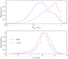 |
Fig. 13 Posterior distributions of the host mass (upper panel) and distance (lower panel) to the lens constructed from the Bayesian analysis. The blue and red curves are the distributions estimated based on the wide and close solutions, respectively. |
Physical lens parameters.
6 Resolving the degeneracy
The degeneracy between the wide and close solutions could have been broken if the peak of the light curve had been covered from followup observations. Due to the high chance of planetary perturbations near the peaks of light curves, high-magnification events were important targets for intensive follow-up observations in the microlensing experiments conducted in a survey+followup mode, in which a survey experiment with a low observational cadence focused on finding events and followup teams, for example, RoboNet (Tsapras et al. 2009), MiNDSTEp (Dominik et al. 2010), μFUN (Gould 2006), and ROME/REA (Tsapras et al. 2019), conducted intensive observations for the alerted events. In this mode of lensing experiments, it was necessary to monitor lensing events found from the survey to select target events for intensive followup observations. This required prodigious human efforts because it was difficult to determine which events would have high magnifications based on the sparse data from the surveys. With the advent of the high-cadence KMTNet survey using globally distributed telescopes, it is now possible to identify high-magnification events with much less efforts for monitoring, enabling followup observations that can increase the number of planets found in high-magnification events, for example, the Earth-mass planet KMT-2020-BLG0414Lb detected from the combined observations by the KMTNet+MOA surveys and LCO & μFUN Follow-Up Team (Zang et al. 2021). Unfortunately, the event KMT-2018-BLG-1743 occurred before the operation of the KMTNet AlertFinder system (Kim et al. 2018), which became fully operational since the 2019 season, and thus a high-magnification alert could not be issued.
Although difficult with the current photometric data, it will be possible to break the degeneracy by resolving the lens and source from future high-resolution imaging observations using HST or AO system mounted on large ground-based telescopes (Bennett et al. 2007). This is possible because the relative lens-source proper motions expected from the wide, μwide ~ 2.3 mas yr−1, and the close, μclose ~ 4.1 mas yr−1, solutions are considerably different from each other. For the case of the planetary lensing event OGLE-2005-BLG-169, the lens and source were resolved from the HST (Bennett et al. 2015) and the Keck AO imaging (Batista et al. 2015) observations, when the lens was separated from the source by ~ 49 mas. Using the same criterion, the lens and source of KMT-2018-BLG-1743 will be separated about 12 yr after the event according to the close solution, that is, in 2030. Unless the lens and source are resolved by that time, the wide solution is more likely to be the correct interpretation of the planetary system. Assuming that the extinction to the lens is approximated as (DL∕DS)AI, where AI ~ 0.84 is the extinction to the source, the expected I-band brightness of the lens is I ~ 23.9 and ~22.8 according to the wide solution and the close solution, respectively.
7 Summary and conclusion
We analyzed the microlensing event KMT-2018-BLG-1743 as part of a project in which anomalous events with no suggested solutions were reinvestigated among the previous lensing events detected in and before the 2019 season by the KMTNet survey. It was found that the light curve of KMT-2018-BLG-1743, which was characterized by a very high peak magnification of Apeak ~ 800 and dual anomalies around the peak and the falling side of the light curve, could not be precisely explained by a 2L1S interpretation. In order to explain the anomalies, we conducted additional modeling with the addition of an extra lens and an extra source to a 2L1S interpretation. From this investigation, we found that 2L2S interpretations with a planetary lens system and a binary source best explained the observed light curve with Δχ2 ~ 188 and ~ 91 over the 2L1S and 3L1S solutions, respectively, giving the event the titles of the fourth 2L2S event and the second 2L2S planetary event. The 2L2S interpretations were subject to a degeneracy, mostly caused by the incomplete coverage of the peak region, resulting in two solutions with s > 1.0 and s < 1.0. It was found that the source was a binary composed of an early G dwarf and a mid M dwarf. The masses of the lens components and the distance to the lens estimated from a Bayesian analysis were (Mhost, Mplanet, DL) ~ (0.19 M⊙, 0.25 MJ, 6.5 kpc) and ~ (0.42 M⊙, 1.61 MJ, 6.0 kpc) according tothe wide and close solutions, respectively. We predicted that the degeneracy between the two solutions would be lifted by resolving the lens and source from future high-resolution imaging observations, due to the considerable difference inthe values of the relative lens-source proper motion expected from the two degenerate solutions.
Acknowledgements
Work by C.H. was supported by the grants of National Research Foundation of Korea (2019R1A2C2085965 and 2020R1A4A2002885). This research has made use of the KMTNet system operated by the Korea Astronomy and Space Science Institute (KASI) and the data were obtained at three host sites of CTIO in Chile, SAAO in South Africa, and SSO in Australia.
References
- Alard, C., & Lupton, R. H. 1998, ApJ, 503, 325 [NASA ADS] [CrossRef] [Google Scholar]
- Albrow, M. 2017, MichaelDAlbrow/pyDIA: Initial Release on Github, Versionv 1.0.0, Zenodo, https://doi.org/10.5281/zenodo.268049 [Google Scholar]
- Albrow, M. D., Beaulieu, J.-P., Caldwell, J. A. R., et al. 2000, ApJ, 534, 894 [Google Scholar]
- Albrow, M., Horne, K., Bramich, D. M., et al. 2009, MNRAS, 397, 2099 [NASA ADS] [CrossRef] [Google Scholar]
- Batista, V., Beaulieu, J.-P., Bennett, D. P., et al. 2015, ApJ, 808, 170B [NASA ADS] [CrossRef] [Google Scholar]
- Becker, A., Alcock, C., Allsman, R., et al. 1997, BAAS, 29, 1347 [Google Scholar]
- Bennett, D. P., Rhie, S. H., Becker, A. C., et al. 1999, Nature, 402, 57 [Google Scholar]
- Bennett, D. P., Anderson, J., & Gaudi, B. S. 2007, ApJ, 660, 781 [NASA ADS] [CrossRef] [Google Scholar]
- Bennett, D. P., Rhie, S. H., Nikolaev, S., et al. 2010, ApJ, 713, 837 [NASA ADS] [CrossRef] [Google Scholar]
- Bennett D. P., Bhattacharya, A., Anderson, J., et al. 2015, ApJ, 808, 169 [Google Scholar]
- Bennett, D. P., Udalski, A., Han, C., et al. 2018, AJ, 155, 141 [Google Scholar]
- Bensby, T., Yee, J. C., Feltzing, S., et al. 2013, A&A, 549, A147 [Google Scholar]
- Bessell, M. S., & Brett, J. M. 1988, PASP, 100, 1134 [NASA ADS] [CrossRef] [Google Scholar]
- Bozza, V., Bachelet, E., Bartolić, F., et al. 2018, MNRAS, 479, 5157 [Google Scholar]
- Claret, A. 2000, A&A, 363, 1081 [NASA ADS] [Google Scholar]
- Dominik, M. 1999, A&A, 349, 108 [NASA ADS] [Google Scholar]
- Dominik, M., & Hirshfeld, A. C. 1994, A&A, 289, L31 [Google Scholar]
- Dominik, M., Jørgensen, U. G., Rattenbury, N. J., et al. 2010, Astron. Nachr., 331, 671 [Google Scholar]
- Dong, S., Bond, I. A., Gould, A., et al. 2009, ApJ, 698, 1826 [NASA ADS] [CrossRef] [Google Scholar]
- Gaudi, B. S., Naber, R. M., & Sackett, P. D. 1998, ApJ, 502, L33 [Google Scholar]
- Gould, A. 1992, ApJ, 392, 442 [NASA ADS] [CrossRef] [EDP Sciences] [Google Scholar]
- Gould, A. 2000, ApJ, 542, 785 [Google Scholar]
- Gould, A., & Gaucherel, C. 1997, ApJ, 477, 580 [Google Scholar]
- Gould, A., Udalski, A., An, D., et al. 2006, ApJ, 644, L37 [NASA ADS] [CrossRef] [Google Scholar]
- Griest, K., & Hu, W. 1993, ApJ, 407, 440 [Google Scholar]
- Griest, K., & Safizadeh, N. 1998, ApJ, 500, 37 [NASA ADS] [CrossRef] [Google Scholar]
- Han, C. 2005, ApJ, 629, 1102 [Google Scholar]
- Han, C. 2006, ApJ, 638, 1080 [NASA ADS] [CrossRef] [Google Scholar]
- Han, C., & Gould, A. 1995, ApJ, 447, 53 [NASA ADS] [CrossRef] [Google Scholar]
- Han, C., & Gould, A. 2003, ApJ, 592, 172 [NASA ADS] [CrossRef] [Google Scholar]
- Han, C., Bennett, D. P., Udalski, A., & Jung, Y. K. 2016, ApJ, 825, 8 [Google Scholar]
- Han, C., Kim, D., Jung, Y. K., et al. 2020a, AJ, 160, 17 [Google Scholar]
- Han, C., Lee, C.-U., Udalski, A., et al. 2020b, AJ, 159, 48 [Google Scholar]
- Han, C., Lee, C.-U., Ryu, Y.-H., et al. 2021a, A&A, 649, 91 [Google Scholar]
- Han, C., Udalski, A., Kim, D., et al. 2021b, AJ, 161, 270 [Google Scholar]
- Han, C., Udalski, A., Lee, C.-U., et al. 2021c, AJ, submitted [Google Scholar]
- Holtzman, J. A., Watson, A. M., Baum, W. A., et al. 1998, AJ, 115, 1946 [NASA ADS] [CrossRef] [Google Scholar]
- Jung, Y. K., Han, C., Gould, A., & Maoz, D. 2013, ApJ, 68, L7 [CrossRef] [Google Scholar]
- Jung, Y. K., Udalski, A., Bond, I. A., et al. 2017, ApJ, 841, 75 [Google Scholar]
- Jung, Y. K., Udalski, A., Gould, A., et al. 2018, AJ, 155, 219 [Google Scholar]
- Jung, Y. K., Han, C., Udalski, A., et al. 2021, AJ, 161, 293 [Google Scholar]
- Kervella, P., Thévenin, F., Di Folco, E., & Ségransan, D. 2004, A&A, 426, 297 [Google Scholar]
- Kim, S.-L., Lee, C.-U., Park, B.-G., et al. 2016, JKAS, 49, 37 [Google Scholar]
- Kim, H.-W., Hwang, K.-H., Shvartzvald, Y., et al. 2018, AAS, submitted [arXiv:1806.07545] [Google Scholar]
- Mao, S., & Paczyński, B. 1991, ApJ, 374, L37 [Google Scholar]
- Nataf, D. M., Gould, A., Fouqué, P., et al. 2013, ApJ, 769, 88 [NASA ADS] [CrossRef] [Google Scholar]
- Paczyński, B. 1986, ApJ, 304, 1 [NASA ADS] [CrossRef] [Google Scholar]
- Robin, A. C., Reylé, C., Derriére, S., & Picaud, S. 2003, A&A, 409, 523 [Google Scholar]
- Tomaney, A. B., & Crotts, A. P. S. 1996, AJ, 112, 2872 [NASA ADS] [CrossRef] [Google Scholar]
- Tsapras, Y., Street, R., Horne, K., et al. 2009, Astron. Nachr., 330, 4 [Google Scholar]
- Tsapras, Y., Street, R. A., Hundertmark, M., et al. 2019, PASP, 131, 124401 [Google Scholar]
- Udalski, A., Szymański, M., Mao, S., et al. 1994, ApJ, 436, L103 [NASA ADS] [CrossRef] [Google Scholar]
- Udalski, A., Jung, Y. K., Han, C., et al. 2015, ApJ, 812, 47 [Google Scholar]
- Yee, J. C., Shvartzvald, Y., Gal-Yam, A., et al. 2012, ApJ, 755, 102 [NASA ADS] [CrossRef] [Google Scholar]
- Yoo, J., DePoy, D. L., Gal-Yam, A., et al. 2004, ApJ, 603, 139 [Google Scholar]
- Zang, W., Han, C., Kondo, I., et al. 2021, Res. Astron. Astrophys., submitted [arXiv:2103.01896] [Google Scholar]
All Tables
All Figures
|
Fig. 1 Light curve of the microlensing event KMT-2018-BLG-1743. The inset shows the zoom-in view of the peak region. The two curves drawn over the data points are the model curves of the 1L1S (dotted) and the wide 2L2S (solid) solutions. The colors of the telescopes in the legend are chosen to match those of the data points in the light curve. |
| In the text | |
|
Fig. 2 Residual from the best-fit model (wide 2L2S model) in various time ranges. The top and middle panels show the residuals in the time ranges of 8165 ≤ HJD′≤ 8420 (225 days) and 8305 ≤HJD′≤ 8323 (18 days), respectively. The bottom panel shows the residual in the time range of 8245 ≤ HJD′≤ 8270 (25 day), during which the source was substantially magnified. |
| In the text | |
|
Fig. 3 Δχ2 map in the logs– logq parameter plane obtained from the 2L1S modeling. Points marked in different colors represent the regions with Δχ2 ≤ n(12) (red), Δχ2 ≤ n(22) (yellow), Δχ2 ≤ n(32) (green), Δχ2 ≤ n(42) (cyan), and Δχ2 ≤ n(52) (blue), where n = 5. The left panel shows the map in the region with − 1.0 < logs ≤ 1.0 and − 5.8 < logq ≤ 0.0, and the right panel shows the map in the narrower region with − 0.26 < logs ≤ 0.26 and − 5.6 < logq ≤−1.9. |
| In the text | |
|
Fig. 4 Lens system configurations of the 2L1S (upper panel) and 3L1S (lower panel) models. In each panel, the inset shows the broad region including the positions of the lens components: blue dots marked by (M1, M2) for the 2L1S model and (M1, M2, M3) for the 3L1S model. The dotted circle in each inset represents the Einstein ring. The source motion is represented by a line with an arrow. The red closed figures represent the caustics. |
| In the text | |
|
Fig. 5 Model curve of the 2L1S solution and the residuals from the model in the central (left panels) and peripheral (right panels) anomaly regions. |
| In the text | |
|
Fig. 6 Δ χ2 maps in the logs3– logq3 (left panel) and log s3–ψ (right panel) planes obtained from the 3L1S grid search. The color coding is same as that in Fig. 3, except that n = 1. |
| In the text | |
|
Fig. 7 Model curve of the 3L1S solution and the residuals from the model. Notations are same as those in Fig. 5. |
| In the text | |
|
Fig. 8 Lens system configurations of the wide (upper panel) and close (lower panel) 2L2S models. Notations are same as those in Fig. 4, except that there are two source trajectories for the primary (S1) and the secondary (S2) source stars. The offset between the arrows on the two source-star trajectories indicates the relative position of the two sources. |
| In the text | |
|
Fig. 9 Model curve of the wide 2L2S solution and the residuals from the model. Notations are same as those in Fig. 5. |
| In the text | |
|
Fig. 10 Model curve of the close 2L2S solution and the residuals from the model. Notations are same as those in Fig. 4. |
| In the text | |
|
Fig. 11 Cumulative distributions of Δχ2 from the 2L1S model for the 3L1S and 2L2S (wide and close) models. The shaded area indicate the central (left) and peripheral (right) anomaly regions. |
| In the text | |
|
Fig. 12 Locations of the primary (S1) and secondary (S2) source stars in the instrumental color-magnitude diagram (CMD). The pair of the filled blue and green dots denote the positions of S1 and S2 based on the wide 2L2S solution, and the pair of the empty dots indicate the positions based on the close 2L2S solution. The red filled dot denotes the centroid of red giant clump (RGC). The HST CMD (brown dots) is presented to show the source locations in the main-sequence branch. |
| In the text | |
|
Fig. 13 Posterior distributions of the host mass (upper panel) and distance (lower panel) to the lens constructed from the Bayesian analysis. The blue and red curves are the distributions estimated based on the wide and close solutions, respectively. |
| In the text | |
Current usage metrics show cumulative count of Article Views (full-text article views including HTML views, PDF and ePub downloads, according to the available data) and Abstracts Views on Vision4Press platform.
Data correspond to usage on the plateform after 2015. The current usage metrics is available 48-96 hours after online publication and is updated daily on week days.
Initial download of the metrics may take a while.