| Issue |
A&A
Volume 652, August 2021
|
|
|---|---|---|
| Article Number | A110 | |
| Number of page(s) | 11 | |
| Section | Planets and planetary systems | |
| DOI | https://doi.org/10.1051/0004-6361/202140563 | |
| Published online | 18 August 2021 | |
Why do more massive stars host larger planets?
1
Center for Theoretical Astrophysics & Cosmology Institute for Computational Science, University of Zurich,
Zurich,
Switzerland
e-mail: This email address is being protected from spambots. You need JavaScript enabled to view it.
2
Department of Planetary Sciences, The University of Arizona,
USA
3
International Space Science Institute,
Bern,
Switzerland
4
Department of Geosciences, Tel-Aviv University,
Tel-Aviv,
Israel
Received:
15
February
2021
Accepted:
18
July
2021
Abstract
Aims. It has been suggested that planetary radii increase with stellar mass for planet sizes smaller than 6 R⊕ and host masses lower than 1 M⊙. In this study, we explore whether this inferred relation of planetary size and host star mass can be explained by a higher planetary mass of planets orbiting higher-mass stars, inflation of the planetary radius due to the difference in stellar irradiation, or different planetary compositions and structures.
Methods. Using exoplanetary data of planets with measured masses and radii, we investigated the relations between stellar mass and various planetary properties for G and K stars. We confirm that more massive stars host larger and more massive planets.
Results. We find that the differences in the planetary masses and temperatures are insufficient to explain the measured differences in radii for planets surrounding different stellar types. We show that the larger planetary radii can be explained by a larger fraction of volatile material (H-He atmospheres) in planets surrounding more massive stars.
Conclusions. We conclude that planets around more massive stars are most probably larger as a result of larger H-He atmospheres. Our findings imply that planets forming around more massive stars tend to accrete H-He atmospheres more efficiently.
Key words: planets and satellites: composition / planets and satellites: terrestrial planets / planets and satellites: interiors / planets and satellites: fundamental parameters
© M. Lozovsky et al. 2021
 Open Access article, published by EDP Sciences, under the terms of the Creative Commons Attribution License (https://creativecommons.org/licenses/by/4.0), which permits unrestricted use, distribution, and reproduction in any medium, provided the original work is properly cited.
1 Introduction
Exoplanetary exploration has led to the discovery of several thousand exoplanets in the past several decades. The interior characterization of these planets has become a key objective in exoplanetary science (e.g., Rogers & Seager 2010; Dorn et al. 2015; Unterborn et al. 2016; Brugger et al. 2017; Owen & Wu 2017; Baumeister et al. 2020; Otegi et al. 2020b). We are now at a stage at which exoplanetary characterization is becoming more detailed, allowing us to understand the various planetary populations within our Galaxy, to link planet formation and evolution models, and to better understand the uniqueness of our own planetary system.
The detected planets with measured radii from the Kepler mission (Borucki et al. 2010) that also have a mass determination using radial velocity (RV) follow-ups or transit-timing variations (TTV) can be used to infer the average density of planets and therefore to estimate the interior composition. We have learned that planets are very diverse astronomical objects and do not follow a single mass-radius (hereafter M-R) relation, but instead show intrinsic scatter (Wolfgang et al. 2015; Chen & Kipping 2016; Ning et al. 2018; Neil & Rogers 2020). This scatter suggests a large diversity in planetary formation and evolution, and also in interior structure and bulk composition (e.g., Weiss & Marcy 2014; Turrini et al. 2015; Petigura et al. 2018; Plotnykov & Valencia 2020). While determining the planetary structure and composition from the measured mass and radius is a highly degenerate problem because very different compositions and structures can yield similar masses and radii (e.g., Rogers & Seager 2010; Dorn et al. 2015, 2017), some trends and limits on the planetary compositions can be found using statistical analysis (e.g., Rogers 2015; Owen & Wu 2017; Lozovsky et al. 2018; Neil & Rogers 2020; Otegi et al. 2020a).
The relatively large database of exoplanets also allows investigating the dependence of the planetary populations on stellar mass (e.g., Fulton & Petigura 2018; Neil & Rogers 2018; Mulders et al. 2015; Pascucci et al. 2018) and metallicity (e.g., Mulders et al. 2016; Mulders 2018; Adibekyan 2019; Kutra & Wu 2020). There are contradictory claims in previous studies about the dependence of Kepler mini-Neptunes and super-Earths on stellar mass. For example, Wu (2019) argued for a linear relation between planetary mass and stellar mass and for no correlation between planet radius and host star metallicity. In contrast, Owen & Murray-Clay (2018) suggested that planetary radii are correlated to stellar metallicity: Stars of higher metallicity host larger planets.
Furthermore, Neil & Rogers (2018) found no strong evidence for a host star mass dependence in the M-R relation using the hierarchical Bayesian modeling approach presented by Wolfgang et al. (2016). Based on this result by Neil & Rogers (2018), Pascucci et al. (2018) applied the Chen & Kipping (2016) M-R relation to convert the planetary radii measured by Kepler into planetary masses. When completeness-corrected occurrence rates were computed versus stellar mass, it was found that the mass of the most common planet for relatively low-mass stars (with masses <1 M⊙) scales almost linearly with stellar mass. Pascucci et al. (2018) showed that the most common planetary mass depends on the mass of the stellar host. More specifically, a universal (i.e., independent of the stellar type) peak in the occurrence rate of the planet-to-star mass ratio for the Kepler planets was found.
Pascucci et al. (2018) focused on MKG stars and suggested that the most common planet around a lower-mass stars is lower in mass. For planets in the radius range of 1–6 R⊕, the Chen & Kipping (2016) M-R relation is presented by a power law. Therefore the Pascucci et al. (2018) data indicate that the most common planet around a lower-mass stars is smaller in radius. Most of the planets in the sample used by Pascucci et al. (2018) have radii larger than 1.6 R⊕ and are therefore likely to have some volatile materials. The addition of these low-density materials (even if very low in terms of mass) can lead to much larger radii for low-mass planets (Rogers 2015; Lozovsky et al. 2018). The M-R relations of planets rich in volatiles are more complex and can vary depending on the planetary temperature and the actual distribution of the material in the interior (e.g., Lozovsky et al. 2018; Mousis et al. 2020; Müller et al. 2020). In addition, it was recently shown that intermediate-mass planets (~5 M⊕ – 20 M⊕) can follow two different M-R relations because they can belong to two different planetary populations (Otegi et al. 2020a).
We here explore potential reasons for the tendency of more massive stars to host larger planets. In principle, at least three explanations are possible for the identified correlation between planetary radius and stellar mass
Case 1: planets are larger due to thermal inflation: because more massive stars are more luminous, higher stellar irradiation might inflate the planetary radius
Case 2: planets around more massive stars are more massive and consequently larger for any given composition.
Case 3: planets around more massive stars tend to be richer in volatiles and are therefore larger.
We investigate these three different cases below. In case 1, we would expect to find a correlation between planetary equilibrium temperature and radius. Case 2 can be examined by testing whether the observed differences in planetary radius can be explained by a variation in planetary mass and case 3 by testing the effect of planetary composition on planetary radius. We discuss the three cases and find that case 3 is the favored interpretation.
2 Methods
We applied a simple statistical analysis of exoplanetary data combined with internal structure models to explore the potential explanations for the observed trend that planets surrounding more massive stars are larger.
The planetary parameters we used in the analysis are the planetary mass, radius, and insolation flux; the stellar parameters are stellar mass, radius, and effective temperature.
First, we built an exoplanetary sample based on the NASA Exoplanet Archive. The planetary sample was used to quantify the differences between different planetary physical properties in exoplanets surrounding different stellar populations.
We next constructed a series of planetary models using structure equations in order to quantify the effect of different parameters, such as planetary mass, temperature, and composition, on the planetary radius (Sect. 2.3) and explored whether the difference in the observed distributions of equilibrium temperatures (case 1) and masses (case 2) is sufficient to explain the difference in the observed radii. Finally, we investigated the effect of various assumed compositions (case 3) on the inferred radii.
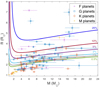 |
Fig. 1 M-R diagram for the planetary sample. The dots with error bars correspond to F planets (purple crosses), G planets (blue squares), K planets (red diamonds), and M planets (yellow pluses). Only G and K planets are used in the analysis. The solid colored curves are M-R relations for various theoretical models with different mass fractions of H-He and constant H2 O mass fraction in the envelope (see Sect. 2.3 for details). The curves correspond to models with a Teq of 700 K (shown as examples). |
2.1 Planetary samples
Our planetary sample is based on the online NASA Exoplanet Archive, which is publicly available. Because we focus on relatively small planets orbiting main sequence stars, we selected transiting planets, with RV or TTV follow-ups with masses Mpl up to 20 M⊕, radii Rpl up to 8 R⊕, and uncertainties on mass and radius of up to 50% of the measured value. We divided the planet samples according to stellar type, which is derived from the stellar effective temperatures (see Table 1). We determined the average radius, mass, and equilibrium temperature (see Sect. 2.1.1 for details) of the planets for each stellar type using the catalog.
Table 1 lists the mean values (μ) and the corresponding standard deviations (σ) calculated assuming a normal distribution. We considered only planets around K and G stars. Hereafter, we refer to planets surrounding G and K stars as “G planets” and “K planets”, respectively. We did not include planets around F stars in our study because F planets do not follow the “universal planet-to-star mass ratio peak” found by Pascucci et al. (2018) and because there are fewer F planets in the planetary sample. M planets are not included either because the planetary database only lists very few of them. The planets we use are listed in the appendix.
The database we used differs from the database used by Pascucci et al. (2018) because the NASA catalog is inhomogeneous in terms of detection methods, measurement uncertainties, and selection effects. While Pascucci et al. (2018) used Kepler planets with well-studied data incompleteness, the NASA database lists planets detected with various methods, such as RV, transit, and direct imagining, and therefore the dataset shows different selections effects and data incompleteness. In addition, by selecting planets withmeasured masses and radii with relatively low uncertainties, we may introduce our own selection. This problem is addressed in Sect. 2.2. The uncertainties of our sample are discussed in Sect. 2.1.2.
Because of the potential biases of our planetary catalog, we explored whether the planet-to-star mass ratio inferred by Pascucci et al. (2018) persists when we used our sample. In order to investigate whether there is a universal peak in the planet-to-star mass ratio, we first calculated the mass ratios for two subsamples, that is, for G and K planets. The distributions of the planet-to-star mass ratio in the two subsamples is shown in Fig. 2, with the distributions’ mean values and peak value qbr from Pascucci et al. (2018). The figure clearly shows that G and K planets have a similar mean value and that this value agrees with qbr inferred by Pascucci et al. (2018). Our results confirm that the mean planetary mass scales with stellar mass.
It is encouraging that despite the large differences in the data and different selection effects, a similar behavior is found. This means that we can use our sample to further investigate the origin of the correlation.
Mean values of planet samples divided by stellar type.
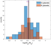 |
Fig. 2 Histogram of the planet-to-star mass ratio for the two subsamples. It can be compared to Fig. 1 of Pascucci et al. (2018). The value of qbr of Pascucci et al. (2018) of log(Mpl∕M*) = −4.55 ± 0.03 is presented as a vertical black line and can be compared with mean values we calculated: − 4.59 ± 0.03 (G planets, red dashed line) and − 4.58 ± 0.04 (K planets, blue dashed line). |
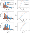 |
Fig. 3 Distributions of planetary radius, mass, and equilibrium temperature of G- and K- planets. The left panels show histograms with the mean values and the corresponding uncertainties (dashed lines). The right panels present the corresponding CDFs. |
2.1.1 Planetary equilibrium temperature
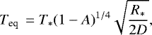
The planetary equilibrium temperatures of the sample are calculated assuming an albedo A = 0. The planetary albedo depends on various parameters, such as atmospheric composition, thermal state, and cloud layers; by assuming zero albedo, corresponding to full absorption, we infer the highest possible equilibrium temperature. The planetary temperature is calculated by
 (1)
(1)
where Teq is planetary equilibrium temperature, T* is the stellar temperature, R* is the stellarradius, and D is the orbital separation. The values for these parameters were taken from the planetary database.
Planets with equilibrium temperatures above 2000 K were not considered because these ultra-hot planets are rare outliers and are likely to be subject to other processes, such as atmospheric loss by photoevaporation (e.g., Rosotti et al. 2013; Jin & Mordasini 2018), which could affect their basic planetary properties. The mean values of Teq, mass, and radius of the samples are listed in Table 1 with the corresponding standard deviations. The distributions of radii, masses, and equilibrium temperatures are presented in Fig. 3.
We performed a Two-sample Kolmogorov–Smirnov test on the subsamples. The test rejects the null hypotheses that masses and radii of G and K planets come from the same distribution at the 5% significance level, and it provides asymptotic p-values of 0.03 and 0.04, respectively. The test did not reject the null hypothesis that the equilibrium temperatures of G and K planets come from the same distribution with an asymptotic p-value of 0.18.
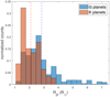 |
Fig. 4 Simulated values of planetary radii accounting for the measurement uncertainties. For each planet in the sample, we simulated 10 000 radii and took the uncertainty into account. The mean values are presented as dashed lines. The histogram of the simulated populations shows the same tendency as the original histogram (see Fig. 3). |
2.1.2 Measurement uncertainties
The planets we included in the samples have small measurement uncertainties, and therefore the planetary mass, radius, and orbital period are rather well constrained. In order to examine the effect of the measurement uncertainties on the main tendency, we performed the test described below.
For each planet in the sample we produced 10 000 synthetic data points using the measured radii and their uncertainties. The simulated values were probed assuming a normal distribution  , where R is the measured radius and Rerr is the corresponding measurement uncertainty. The simulated values are presented in Fig. 4. It shows that the main trend of more massive stars hosting larger planets persists.
2.2 Selection effects
Most of the detected exoplanets with measured radii were observed with the Kepler mission using the transit method, where the transit depth is given by
 (2)
(2)
Here dF is the dimming due to the transit, and Fst is the stellarflux (e.g., Bozza et al. 2016). As a result, smaller planets are easier to detect around smaller stars but are easier to miss aroundlarger stars. This might introduce an artificial correlation between planetary size and stellar size (or stellar mass).
In order to test whether our sample shows a strong selection effect of this kind, we compared our sample withthe wider (and homogeneous) sample of Kepler and K2 planets using the NASA catalog, without anyrestriction on a planetary mass. Specifically, we selected planets with sizes up to 8 R⊕ and uncertainties below 50% of the measured values that surround G and K stars with measured stellar radii and temperatures.
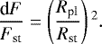
Figure 5 shows the planetary radius as a function of the planet-to-star radius ratio squared  . In this figure, the full sample consisting of 1267 G planets and 643 K. In contrast to the expectation from a transit-depth-related selection bias, neitherthe full Kepler sample nor our subsample show a lack of detected planets below some critical transit depth, that is, a vertical cutoff in
  . Both G and K stars in our subsample appear to host planets as small as 1.2–1.4 R⊕. In addition, our subsample has planet-to-star radius ratios significantly larger than the minimal value of ~ 3 × 10⁻⁵ in the full sample. This suggests that selection effects due to small transit depths are unlikely to affect the main results of this study.
 |
Fig. 5 Planetary radius vs. the square of the planet-to-star radius ratio |

2.3 Interior modeling
In order to explain the observed differences in planetary properties of different populations, we inferred the relation between theplanetary mass and radius (M-R relations) for planets with different assumed compositions and internal structures. It is reasonable to model the planets in the samples with volatile-rich interiors because most of them have larger radii than expected for an Earth-like composition (e.g., Rogers 2015; Lozovsky et al. 2018). The planetary structure models we used consist of a rocky core surrounded by a hydrogen-helium (H-He) and a water (H2 O) envelope. For simplicity, the composition of the core was set to be pure MgSiO3. More complex core structures are expected to have a negligible effect on the M-R relation for volatile-rich planets (Howe et al. 2014; Otegi et al. 2020a). The H-to-He ratio was assumed to be protosolar, that is, 72% H to 28% He by mass, and the water mass fraction was taken to be 20% in the envelope (water + H-He). The equation of state for H-He was taken from Saumon et al. (1995), for MgSiO3 from Seager et al. (2007), and for H2O from Vazan et al. (2013). The atmospheric models were derived using the standard structural equations of hydrostatic equilibrium, mass conservation, and heat transport. We followed the irradiation model of Guillot (2010) for the H-He envelope. Further details on the structure models can be found in Venturini et al. (2015), Dorn et al. (2017), and Lozovsky et al. (2018) and references therein. We considered two cases of envelope structure: a homogeneously mixed envelope consisting of H-He and water, and a differentiated structure in which water and H-He are separated and the pure water layer is below pure H-He layer. The first case (homogeneous envelope) was used as default.
The structure models were constructed assuming various percentages of H-He of between 0.5 and 25% of the total planetary mass and different equilibrium temperatures Teq (see Sect. 2.1.1 for details). Models with H-He mass fractions larger than 25% were not considered because we focus on planets up to 20 M⊕, which are unlikely to be H-He-rich. The M-R relations together with the planetary sample are shown in Fig. 1. The curves presented in this plot are examples assuming Teq = 700 K. The calculated M-R relations allow us to derive the planetary radius corresponding to any given mass and Teq. These models are used in the following analysis in order to investigate the potential reason(s) for the trend that larger planets are located around more massive stars.
3 Results
3.1 Case 1: larger planets through inflation
As mentioned above, most of the planets in the sample are expected to be rich in volatiles given their large radii and low bulk densities (Fig. 6). Radii of volatile-rich planets are very sensitive to the temperature: planets with the same mass, chemical composition, and internal structure can have different radii for different temperatures because of thermal inflation. Planets surrounding more massive stars seem to be slightly hotter on average (see Fig. 3). Therefore it is reasonable to expect that the differences in the equilibrium temperatures for G and K planets could lead to differences in radii of the two populations. We use the planet sample below to evaluate any possible correlation between planetary equilibrium temperatures and radii.
Figure 6 (upper panel) presents the observed planetary radii versus equilibrium temperature Teq, calculated from Eq. (1). Interestingly, the observed radii do not increase with temperature. G and K planets even tend to have smaller radii at higher temperatures. Figure 6 (lower panel) presents the bulk densities (inferred from the measured masses and radii) versusTeq for the detected planets. No significant decrease in bulk density with temperature is observed. In the contrary, the bulk densities of both G and K planets increase with temperature, suggesting that very hot planets tend to be more rocky. This correlation could be a result of atmospheric mass loss of primordial hydrogen-atmospheres, which depends on stellar insolation (Fulton & Petigura 2018; Owen & Wu 2017; Jin & Mordasini 2018).
This shows that the observed radii do not correlate with temperature, and thermal inflation does not play a significant role in the observed trend. We therefore conclude that the differences in the equilibrium temperature alone are insufficient to explain the differences in the observed radii of the two planetary populations.
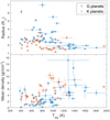 |
Fig. 6 Measured planetary radius (upper panel) and calculated planetary bulk density (lower panel) vs. calculated equilibrium temperature for our sample of planets. |
3.2 Case 2: larger planets through a higher planetary mass
When we assume that the planetary radius scales with mass, it is reasonable to expect that the observed difference in radii is a result of thedifference in planetary mass. In this section we investigate whether the observed difference in average radii is caused by more massive planets around more massive stars.
To investigate this option, we used the theoretical M-R relations of planets with rocky cores surrounded by H-He + H2 O atmospheres, calculated from the internal structure models described in Sect. 2.3. The typical difference between masses of G planets and K planets in the sample is ~2 M⊕. The mass difference is calculated as a difference between the mean values of the distributions. This difference in mass distributions (see Fig. 3 and Table 1) is insufficient to explain the difference in the observed radii of 0.75 R⊕ because the M-R curves are very flat in this regime (Lopez & Fortney 2014; Weiss et al. 2013; Wolfgang et al. 2015; Chen & Kipping 2016; Lozovsky et al. 2018). This implies a weak dependence of the radius for these planetary masses.
In order to test whether the difference in radii is a result of different planetary masses, we calculated the radius corresponding to a hypothetical average mass planet of each stellar type: 9.41 M⊕ for G planets and 7.33 M⊕ for K planets, as listed in Table 1. To isolate the effect of mass, we assumed a uniform temperature of Teq = 900 K and H-He mass fraction of 2% for both hypothetical planets. This method compares the mean values of the mass distributions, as we are assuming that the average masses are representative of the main trend. By calculating a radius corresponding to each average mass and using the same M-R relation and temperature for all of the masses, we are able to isolate the effect of the mass alone. The calculated radii of both G planets and K planets are found to be in the range of 2.62–2.76 R⊕ for G planets and 2.58–2.81 R⊕ for K planets. These radii ranges were calculated assuming two different atmospheric structures. The lower radius boundary was calculated assuming a homogeneous envelope structure (water and H-He are mixed), while the upper limit was calculated assuming a differentiated structure in which water and H-He are separated (see Sect. 2.3). We find that the effect of the mass on the calculated radius alone is negligible compared to the observed differences.
Therefore we conclude that the difference in the planetary masses cannot explain the measured difference in planetary radii.
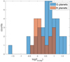 |
Fig. 7 Histogram of simulated fH-He for our planetary samples. Planets that cannot be modeled with any H-He mass fraction are not presented. |
3.3 Case 3: larger planets through different compositions
Finally, we investigated the effect of different compositions and envelope structures on the planetary radius. For planets with thick H-He envelopes, the planetary structure and exact H-He mass fraction have significant effects on the M-R relation (see Lozovsky et al. 2018 for details). For the same planetary mass and temperature, the difference between a planet with fH-He of 0.5 and fH-He of 10% is between ~1.2 R⊕ and ~ 1.8 R⊕. This range exceeds the difference between the measured radii of G and K planets: the difference between the peaks of the radii distribution is 0.75 R⊕.
We next compare the radii inferred when assuming various compositions and internal structures with the measured ones. Using the planetary models described in Sect. 2.3, we calculated for each planet the corresponding fH-He. The calculation uses the planetary effective temperature and the measured mass. The results are shown in Fig. 7. There is a clear trend where planets around more massive stars have higher fH-He values. G planets have0 ≲ fH-He ≲ 0.4, and K planets have0 ≲ fH-He ≲ 0.15), with mean values of 0.06 ± 0.01 and 0.03 ± 0.01, respectively.Several small planets are unlikely to consist of H-He: this corresponds to 15 G planets and 15 K planets. These planets are probably rocky water-dominated planets without any significant volatile atmosphere, and they therefore their radii do not strongly depend on Teq and accordingly do not affect our conclusions. These planets are not presented in Fig. 7. In Fig. 1 they are located below the 0.5% H-He line.
As expected, the H-He mass fraction in the planet fH-He has a crucial effect on the inferred radii (e.g., Fig. 1; Swift et al. 2012; Weiss & Marcy 2014). The difference in the assumed fH-He leads to a radius difference that can exceed the difference between G planets and K planets. We therefore suggest thatthe difference in observed radii of planets orbiting stars with different masses could be caused by different H-He mass fractions, with the G planets being more volatile-rich in comparison to K planets. In addition, the distribution of volatiles has a significant effect on M-R relations: the size difference between fully differentiated and homogeneous envelopes is larger than the difference due to thermal inflation and higher mass (e.g., Soubiran & Militzer 2015).
We conclude that while case 1 (thermal inflation) and case 2 (higher mass) cannot explain the observed differences, case 3 (different planetary composition and structure) can explain the observations.
4 Discussion
We investigate the potential explanations for the observed correlation between mean planetary size and stellar type. We showed that different H-He mass fractions could explain this observations. In the analysis, we restricted the possible theoretical models to a rather narrow range: rocky cores surrounded by H-He+H2O atmospheres, with fH-He = 0.5−25% and a water fraction in the envelope of 20% by mass. Nevertheless, even in this narrow assumption range, we were able to provide an interpretation for the reason that the most typical planetary radius scales with stellar mass. We suggest that this correlation might be the result of characteristically different planetary composition and/or structure of the planets that surround different stellar types, while planetary mass and insolation are unlikely to affect this relation strongly. Planet formation and evolution models could confirm this idea. In addition, it is unlikely that the correlation we found is caused by data incompleteness. Nevertheless, the planetary data we used in this analysis are somewhat limited and inhomogeneous. As a result, it is desirable to use larger samples in the future and repeat the analysis accounting for a wider range in stellar spectral types, also including M dwarfs.
Previous studies have investigated differences in planet populations between M dwarfs and FGK dwarfs. Giant planets are scarce around M dwarfs (Bonfils et al. 2013), and there is a higher occurrence of small planets around M dwarfs (Dressing & Charbonneau 2015; Gaidos et al. 2016). The higher planet-formation efficiency of low-mass stars (Dai et al. 2020) may be related to the low giant planet occurrence or the longer disk lifetimes, or to other factors. The difference in planetary composition distribution is unclear so far. No strong evidence for a dependence of the planetary M-R relation on host star mass for small planets has been reported (Neil & Rogers 2018). If extrapolated to M dwarfs, our findings would predict a tendency of H-He-poor planets compared to those around more massive stars. This is somewhat in line with previous studies (Bonfils et al. 2013; Dressing & Charbonneau 2015; Gaidos et al. 2016) because planets around M stars are less massive. This does not imply that planets are poor in water. In fact, planets around M dwarfs can be rich in water as a result of an efficient inward migration (Alibert & Benz 2017; Burn et al. 2021).
Kepler planets are located relatively close to their stars and may thus be affected by planet–star interactions, either by stellar insolation during planet evolution or during formation in the protoplanetary disk. Here, we argue that stellar insolation alone cannot compensate for the different radii in the observed planetary populations around G and K stars. Instead we provide evidence that the populations are different through their formation processes, that is, the efficiency of envelope accretion. This can be a result of more massive protoplanetary disks (Mohanty et al. 2013; Andrews et al. 2013; Pascucci et al. 2016; Ansdell et al. 2016) that lead to faster growth (Hartmann et al. 2006; Alcalá et al. 2014) followed by H-He accretion (even if in small amounts), and/or due to different disk lifetimes (Ribas et al. 2015). Essentially, core growth is more efficient both in higher-mass disks (Mordasini et al. 2012; Venturini et al. 2020) and around higher-mass stars (Kennedy & Kenyon 2008), allowing them to to accrete a substantial gaseous envelope before the gas disk dissipates.
The diversity of planetary envelopes of our sample is unknown so far, and different compositions including H, He, water, and higher mean molecular species are possible. In addition to compositional diversity, these planets may absorb stellar energy differently, which affects their thermal structure and thus their radii.
In this regard, it would be desirable to investigate the dependence on the assumed albedo. We here assumed a uniform zero albedo for all planets when we calculated Teq. Because different compositions can lead to different albedos, the relation between the different parameters is likely to be very complex. Another important property that might affect the planetary population is the age of the system. In order to investigate the correlation between the age and size of the planets, we need better constraints on the stellar ages. These are not available for most of the stars in current planetary databases.
It should be noted that planets around F stars are not included in this analysis because they do not present the same tendency as G and K planets, as was shown by Pascucci et al. (2018). F stars are more luminous, and as a result, they are causing higher irradiation. Close-in planets might accordingly undergo other physical effects, such as atmospheric loss by photoevaporation (e.g., Rosotti et al. 2013; Jin & Mordasini 2018), which might affect their basic planetary properties and alter the statistics. It is therefore clear that more data and theoretical models that account for the planetary evolution are required before a conclusion can be reached regarding the expected compositions of planets around F stars.
5 Summary and conclusions
We confirm that planets surrounding more massive stars tend to be higher in mass and larger in radius. In this study we investigated the effect of the planetary mass, equilibrium temperature, and possible bulk composition on the planetary radius for planets surrounding G and K stars. The larger radii of planets surrounding more massive stars cannotbe explained by inflation through higher irradiation of the star, nor by a higher planetary mass: the effect of both properties on the radius was found to be significantly smaller than the observed difference. In other words, we showed that the difference in planetary mass that is given by RV/TTV data is insufficient to explain the observed difference in planetary radii, and the planetary temperature is even found to be anticorrelated with radius.
Larger H-He mass fractions on planets around more massive stars can easily explain the trends in the observed data.We therefore suggest that the larger radii of planets surrounding more massive stars are a result of different compositions: more massive stars tend to host planets with larger H-He mass fractions. If this is correct, it provides important constraints for planet formation models because it implies that planets forming around more massive stars tend to accrete H-He atmospheres more efficiently. This can be the result of more massive protoplanetary disks that lead to faster core growth, allowing the cores to accrete substantial gaseous envelopes before the gas disk dissipates. We therefore argue that planets around G and K stars are different by formation.
In this light, it is desirable to have further constraints available to test our findings. Further information on the planetary composition would come from the James Webb Space Telescope and Ariel missions with constraints on atmospheric composition, which will shed more light on the diversity of planetary volatile envelopes, their formation efficiencies, and their evolution. In addition, an important property of a planetary system is the planetary age, which is typically not very well constrained (e.g., Saffe et al. 2005; Silva Aguirre et al. 2015; Guillot et al. 2014). This is expected to change with the PLATO mission, which will allow estimating the stellar ages with accuracies of about 10% (Rauer et al. 2014). With age constraints, we will be able to determine if and how the discussed differences in planet populations evolve in time.
Acknowledgements
R.H. acknowledges support from SNSF grant 200021_169054. C.D. acknowledges support from the Swiss National Science Foundation under grant PZ00P2_174028. This work has been carried out within the frame of the National Center for Competence in Research PlanetS supported by the SNSF Swiss National Foundation.
Appendix A Tables of planetary data
Planets used in the study
References
- Adibekyan, V. 2019, Geosciences, 9, 105 [NASA ADS] [CrossRef] [Google Scholar]
- Alcalá, J. M., Natta, A., Manara, C. F., et al. 2014, A&A, 561, A2 [NASA ADS] [CrossRef] [EDP Sciences] [Google Scholar]
- Alibert, Y., & Benz, W. 2017, A&A, 598, L5 [NASA ADS] [CrossRef] [EDP Sciences] [Google Scholar]
- Andrews, S. M., Rosenfeld, K. A., Kraus, A. L., & Wilner, D. J. 2013, ApJ, 771, 129 [Google Scholar]
- Ansdell, M., Williams, J. P., van der Marel, N., et al. 2016, ApJ, 828, 46 [Google Scholar]
- Baumeister, P., Padovan, S., Tosi, N., et al. 2020, ApJ, 889, 42 [CrossRef] [Google Scholar]
- Bonfils, X., Delfosse, X., Udry, S., et al. 2013, A&A, 549, A109 [NASA ADS] [CrossRef] [EDP Sciences] [Google Scholar]
- Borucki, W. J., Koch, D., Basri, G., et al. 2010, Science, 327, 977 [NASA ADS] [CrossRef] [PubMed] [Google Scholar]
- Bozza, V., Mancini, L., Sozzetti, A., et al. 2016, Astrophys. Space Sci. Lib., 428 [Google Scholar]
- Brugger, B., Mousis, O., Deleuil, M., & Deschamps, F. 2017, ApJ, 850, 93 [Google Scholar]
- Burn, R., Schlecker, M., Mordasini, C., et al. 2021, A&A in press, https://doi.org.10.1051/0004-6361/202140390 [Google Scholar]
- Chen, J., & Kipping, D. 2016, ApJ, 834, 17 [NASA ADS] [CrossRef] [Google Scholar]
- Dai, F., Winn, J. N., Schlaufman, K., et al. 2020, AJ, 159, 247 [Google Scholar]
- Dorn, Amir, K., Heng, K., et al. 2015, A&A, 577, A83 [EDP Sciences] [Google Scholar]
- Dorn, C., Venturini, J., Khan, A., et al. 2017, A&A, 597, A37 [NASA ADS] [CrossRef] [EDP Sciences] [Google Scholar]
- Dressing, C. D., & Charbonneau, D. 2015, ApJ, 807, 45 [NASA ADS] [CrossRef] [Google Scholar]
- Fulton, B. J., & Petigura, E. A. 2018, AJ, 156, 264 [Google Scholar]
- Gaidos, E., Mann, A. W., Kraus, A. L., & Ireland, M. 2016, MNRAS, 457, 2877 [Google Scholar]
- Guillot, T. 2010, A&A, 520, A27 [NASA ADS] [CrossRef] [EDP Sciences] [Google Scholar]
- Guillot, T., Lin, D., Morel, P., Havel, M., & Parmentier, V. 2014, Euro. Astron. Soc. Pub. Ser., 65, 327 [NASA ADS] [Google Scholar]
- Hartmann, L., D’Alessio, P., Calvet, N., & Muzerolle, J. 2006, ApJ, 648, 484 [Google Scholar]
- Howe, A. R., Burrows, A., & Verne, W. 2014, ApJ, 787, 173 [NASA ADS] [CrossRef] [Google Scholar]
- Jin, S., & Mordasini, C. 2018, ApJ, 853, 163 [Google Scholar]
- Kennedy, G. M., & Kenyon, S. J. 2008, ApJ, 673, 502 [NASA ADS] [CrossRef] [Google Scholar]
- Kutra, T., & Wu, Y. 2020, AJ, submitted [arXiv:2003.08431] [Google Scholar]
- Lopez, E. D., & Fortney, J. J. 2014, ApJ, 792, 1 [NASA ADS] [CrossRef] [Google Scholar]
- Lozovsky, M., Helled, R., Dorn, C., & Venturini, J. 2018, ApJ, 866, 49 [Google Scholar]
- Mohanty, S., Greaves, J., Mortlock, D., et al. 2013, ApJ, 773, 168 [NASA ADS] [CrossRef] [Google Scholar]
- Mordasini, C., Alibert, Y., Benz, W., Klahr, H., & Henning, T. 2012, A&A, 541, A97 [NASA ADS] [CrossRef] [EDP Sciences] [Google Scholar]
- Mousis, O., Deleuil, M., Aguichine, A., et al. 2020, ApJ, 896, L22 [Google Scholar]
- Mulders, G. D. 2018, Planet Populations as a Function of Stellar Properties (Cham: Springer International Publishing), 1 [Google Scholar]
- Mulders, G. D., Pascucci, I., & Apai, D. 2015, ApJ, 798, 112 [Google Scholar]
- Mulders, G. D., Pascucci, I., Apai, D., Frasca, A., & Molenda-Żakowicz, J. 2016, AJ, 152, 187 [NASA ADS] [CrossRef] [Google Scholar]
- Müller, S., Ben-Yami, M., & Helled, R. 2020, ApJ, 903, 147 [CrossRef] [Google Scholar]
- Neil, A. R., & Rogers, L. A. 2018, ApJ, 858, 58 [NASA ADS] [CrossRef] [Google Scholar]
- Neil, A. R., & Rogers, L. A. 2020, ApJ, 891, 12 [Google Scholar]
- Ning, B., Wolfgang, A., & Ghosh, S. 2018, ApJ, 869, 5 [NASA ADS] [CrossRef] [Google Scholar]
- Otegi, J., Bouchy, F., & Helled, R. 2020a, A&A, 634, A43 [NASA ADS] [CrossRef] [EDP Sciences] [Google Scholar]
- Otegi, J. F., Dorn, C., Helled, R., et al. 2020b, A&A, 640, A135 [NASA ADS] [CrossRef] [EDP Sciences] [Google Scholar]
- Owen, J. E., & Murray-Clay, R. 2018, MNRAS, 480, 2206 [CrossRef] [Google Scholar]
- Owen, J. E., & Wu, Y. 2017, ApJ, 847, 29 [Google Scholar]
- Pascucci, I., Testi, L., Herczeg, G. J., et al. 2016, ApJ, 831, 125 [Google Scholar]
- Pascucci, I., Mulders, G. D., Gould, A., & Fernandes, R. 2018, ApJ, 856, L28 [NASA ADS] [CrossRef] [Google Scholar]
- Petigura, E. A., Marcy, G. W., Winn, J. N., et al. 2018, AJ, 155, 89 [NASA ADS] [CrossRef] [Google Scholar]
- Plotnykov, M., & Valencia, D. 2020, MNRAS, 499, 932 [Google Scholar]
- Rauer, H., Catala, C., Aerts, C., et al. 2014, Exp. Astron., 38, 249 [Google Scholar]
- Ribas, Á., Bouy, H., & Merín, B. 2015, A&A, 576, A52 [NASA ADS] [CrossRef] [EDP Sciences] [Google Scholar]
- Rogers. 2015, ApJ, 801, 41 [NASA ADS] [CrossRef] [Google Scholar]
- Rogers, & Seager, S. 2010, ApJ, 712, 974 [NASA ADS] [CrossRef] [Google Scholar]
- Rosotti, G. P., Ercolano, B., Owen, J. E., & Armitage, P. J. 2013, MNRAS, 430, 1392 [NASA ADS] [CrossRef] [Google Scholar]
- Saffe, C., Gómez, M., & Chavero, C. 2005, A&A, 443, 609 [NASA ADS] [CrossRef] [EDP Sciences] [Google Scholar]
- Saumon, D., Chabrier, G., & van Horn, H. M. 1995, ApJS, 99, 713 [Google Scholar]
- Seager, S., Kuchner, M., Hier-Majumder, C. A., & Militzer, B. 2007, ApJ, 669, 1279 [Google Scholar]
- Silva Aguirre, V., Davies, G. R., Basu, S., et al. 2015, MNRAS, 452, 2127 [NASA ADS] [CrossRef] [Google Scholar]
- Soubiran, F., & Militzer, B. 2015, ApJ, 806, 228 [NASA ADS] [CrossRef] [Google Scholar]
- Swift, D. C., Eggert, J. H., Hicks, D. G., et al. 2012, ApJ, 744, 59 [NASA ADS] [CrossRef] [Google Scholar]
- Turrini, D., Nelson, R. P., & Barbieri, M. 2015, Exp. Astron., 40, 501 [NASA ADS] [CrossRef] [Google Scholar]
- Unterborn, C. T., Dismukes, E. E., & Panero, W. R. 2016, ApJ, 819, 32 [Google Scholar]
- Vazan, A., Kovetz, A., Podolak, M., & Helled, R. 2013, MNRAS, 434, 3283 [Google Scholar]
- Venturini, J., Alibert, Y., Benz, W., & Ikoma, M. 2015, A&A, 576, A114 [NASA ADS] [CrossRef] [EDP Sciences] [Google Scholar]
- Venturini, J., Guilera, O. M., Ronco, M. P., & Mordasini, C. 2020, A&A, 644, A174 [Google Scholar]
- Weiss, L. M., & Marcy, G. W. 2014, ApJ, 783, L6 [NASA ADS] [CrossRef] [Google Scholar]
- Weiss, L. M., Marcy, G. W., Rowe, J. F., et al. 2013, ApJ, 768, 14 [NASA ADS] [CrossRef] [Google Scholar]
- Wolfgang, A., Rogers, L. A., & Ford, E. B. 2015, Proc. Int. Astron. Union, 11, 223 [CrossRef] [Google Scholar]
- Wolfgang, A., Rogers, L. A., & Ford, E. B. 2016, ApJ, 825, 19 [Google Scholar]
- Wu, Y. 2019, ApJ, 874, 91 [NASA ADS] [CrossRef] [Google Scholar]
All Tables
All Figures
|
Fig. 1 M-R diagram for the planetary sample. The dots with error bars correspond to F planets (purple crosses), G planets (blue squares), K planets (red diamonds), and M planets (yellow pluses). Only G and K planets are used in the analysis. The solid colored curves are M-R relations for various theoretical models with different mass fractions of H-He and constant H2 O mass fraction in the envelope (see Sect. 2.3 for details). The curves correspond to models with a Teq of 700 K (shown as examples). |
| In the text | |
|
Fig. 2 Histogram of the planet-to-star mass ratio for the two subsamples. It can be compared to Fig. 1 of Pascucci et al. (2018). The value of qbr of Pascucci et al. (2018) of log(Mpl∕M*) = −4.55 ± 0.03 is presented as a vertical black line and can be compared with mean values we calculated: − 4.59 ± 0.03 (G planets, red dashed line) and − 4.58 ± 0.04 (K planets, blue dashed line). |
| In the text | |
|
Fig. 3 Distributions of planetary radius, mass, and equilibrium temperature of G- and K- planets. The left panels show histograms with the mean values and the corresponding uncertainties (dashed lines). The right panels present the corresponding CDFs. |
| In the text | |
|
Fig. 4 Simulated values of planetary radii accounting for the measurement uncertainties. For each planet in the sample, we simulated 10 000 radii and took the uncertainty into account. The mean values are presented as dashed lines. The histogram of the simulated populations shows the same tendency as the original histogram (see Fig. 3). |
| In the text | |
|
Fig. 5 Planetary radius vs. the square of the planet-to-star radius ratio |
| In the text | |
|
Fig. 6 Measured planetary radius (upper panel) and calculated planetary bulk density (lower panel) vs. calculated equilibrium temperature for our sample of planets. |
| In the text | |
|
Fig. 7 Histogram of simulated fH-He for our planetary samples. Planets that cannot be modeled with any H-He mass fraction are not presented. |
| In the text | |
Current usage metrics show cumulative count of Article Views (full-text article views including HTML views, PDF and ePub downloads, according to the available data) and Abstracts Views on Vision4Press platform.
Data correspond to usage on the plateform after 2015. The current usage metrics is available 48-96 hours after online publication and is updated daily on week days.
Initial download of the metrics may take a while.