| Issue |
A&A
Volume 652, August 2021
|
|
|---|---|---|
| Article Number | A7 | |
| Number of page(s) | 10 | |
| Section | Cosmology (including clusters of galaxies) | |
| DOI | https://doi.org/10.1051/0004-6361/202039895 | |
| Published online | 30 July 2021 | |
TDCOSMO
VI. Distance measurements in time-delay cosmography under the mass-sheet transformation
1
Department of Physics and Astronomy, University of California, Davis, CA 95616, USA
e-mail: gcfchen@astro.ucla.edu
2
Max Planck Institute for Astrophysics, Karl-Schwarzschild-Strasse 1, 85740 Garching, Germany
3
Physik-Department, Technische Universität München, James-Franck-Straße 1, 85748 Garching, Germany
4
Academia Sinica Institute of Astronomy and Astrophysics (ASIAA), 11F of ASMAB, No. 1, Section 4, Roosevelt Road, Taipei 10617, Taiwan
5
Kavli IPMU (WPI), UTIAS, The University of Tokyo, Kashiwa, Chiba 277-8583, Japan
6
Department of Physics and Astronomy, Johns Hopkins University, 3400 North Charles Street, Baltimore, MD 21218, USA
Received:
12
November
2020
Accepted:
26
March
2021
Time-delay cosmography with gravitationally lensed quasars plays an important role in anchoring the absolute distance scale and hence measuring the Hubble constant, H0, independent of traditional distance ladder methodology. A current potential limitation of time-delay distance measurements is the mass-sheet transformation (MST), which leaves the lensed imaging unchanged but changes the distance measurements and the derived value of H0. In this work we show that the standard method of addressing the MST in time-delay cosmography, through a combination of high-resolution imaging and the measurement of the stellar velocity dispersion of the lensing galaxy, depends on the assumption that the ratio, Ds/Dds, of angular diameter distances to the background quasar and between the lensing galaxy and the quasar can be constrained. This is typically achieved through the assumption of a particular cosmological model. Previous work (TDCOSMO IV) addressed the mass-sheet degeneracy and derived H0 under the assumption of the ΛCDM model. In this paper we show that the mass-sheet degeneracy can be broken without relying on a specific cosmological model by combining lensing with relative distance indicators such as supernovae Type Ia and baryon acoustic oscillations, which constrain the shape of the expansion history and hence Ds/Dds. With this approach, we demonstrate that the mass-sheet degeneracy can be constrained in a cosmological model-independent way. Hence model-independent distance measurements in time-delay cosmography under MSTs can be obtained.
Key words: distance scale / gravitational lensing: strong
© ESO 2021
1. Introduction
The Hubble constant (H0) is one of the most important parameters in cosmology. Its value directly sets the age, size, and critical density of the Universe. Despite the great success of the Λ cold dark matter (CDM) model (Komatsu et al. 2011; Hinshaw et al. 2013; Planck Collaboration VI 2020), a stringent challenge to the model comes from a discrepancy between the extremely precise H0 (= 67.4 ± 0.5 km s−1 Mpc−1) value derived from Planck measurements of the cosmic microwave background (CMB) anisotropies under the assumption of ΛCDM (Planck Collaboration VI 2020) and the H0 value from direct measurements of the local Universe (Verde et al. 2019).
The recent direct H0 measurements (H0 = 74.03 ± 1.42 km s−1 Mpc−1) from Type Ia supernovae (SN1a), calibrated by the traditional Cepheid distance ladder (SH0ES collaboration; Riess et al. 2019), show a 4.4σ tension with the Planck results. However, a recent measurement of H0 = 69.8 ± 0.8(stat) ± 1.7(sys) km s−1 Mpc−1 from SN1a calibrated by the tip of the red giant branch (CCHP) agrees at the 1.2σ level with Planck and at the 1.7σ with the SH0ES results (Freedman et al. 2019). The spread in these results, whether due to systematic effects (Efstathiou 2020) or not, clearly demonstrates that it is crucial to test any single methodology by different and independent datasets.
Time-delay cosmography (TDC; e.g., Treu & Marshall 2016; Suyu et al. 2018) provides a technique to constrain H0 at low redshift that is completely independent of the traditional distance ladder approach. When a quasar is strongly lensed by a galaxy, its multiple images have light curves that are offset by a well-defined time delay, which depends on the mass profile of the lens and cosmological distances to the galaxy and quasar (Refsdal 1964). A critical aspect of this technique is a model that describes the mass distribution in the lensing galaxy and along the line of sight between the background object and the observer. This model is constrained by the morphology of the lensed emission of the background object, the stellar velocity dispersion in the lensing galaxy, and by deep imaging and spectroscopy of the fields containing the lens system. This model is combined with the time delays (e.g., Bonvin et al. 2018) to measure the characteristic distances for the lens system: the angular diameter distance to the lens (Dd) and the time-delay distance, which is a ratio of the angular diameter distances in the system, as follows:
where zd is the redshift of the lens, Ds is the distance to the background source, and Dds is the distance between the lens and the source. In turn, these distances are used to determine cosmological parameters, primarily H0 (e.g., Suyu et al. 2014; Bonvin et al. 2016; Birrer et al. 2019; Chen et al. 2019; Rusu et al. 2019; Wong et al. 2019; Jee et al. 2019; Taubenberger et al. 2019; Shajib et al. 2020).
A recent analysis with this technique, using a blind analysis on data from six gravitational lens systems1, inferred  , which is a value that was 3.8σ offset from the Planck results (Wong et al. 2019; Millon et al. 2020). This analysis used two common descriptions of the mass distribution of the lensing galaxy. The first description consists of a NFW halo (Navarro et al. 1996) plus a constant mass-to-light ratio stellar distribution, called the composite model. The second description models the 3D total mass density distribution, that is, luminous plus dark matter, of the galaxy as a power law ( i.e., ρ(r) ∝ r−γ; Barkana 1998); this description is called the power-law model. These models yield H0 measurements that are consistent within the errors for individual lens systems; the final uncertainties on H0 incorporate a marginalization over the choice of mass model (Millon et al. 2020).
Although the power-law and composite models are well-motivated by observations (e.g., Koopmans et al. 2006, 2009; Suyu et al. 2009; Auger et al. 2010; Barnabè et al. 2011; Sonnenfeld et al. 2013; Humphrey & Buote 2010; Cappellari 2016) and simulations (Navarro et al. 1996), there is a well-known degeneracy in gravitational lensing known as the mass-sheet transformation (MST). The MST leaves imaging observables invariant, but biases the determination of H0 (Falco et al. 1985; Gorenstein et al. 1988). The line-of-sight mass distribution contributes to first order mass-sheet-like effect (Fassnacht et al. 2002; Suyu et al. 2013; Greene et al. 2013; Collett et al. 2013); we refer to this as an external MST. However, for the mass distribution of the lensing galaxy, there are different models that can give the same lensing observables, but would give different time delays. The most degenerate case is that with spherical symmetry, in which the density profiles differ by a component that is uniform in within the radial ranges probed by lensing. This component, which could be described by a large-core mass distribution (Blum et al. 2020, see detail in Sect. 2), changes the distribution of the mass density profile of the lensing galaxy. This fits with recent works that question whether that elliptical galaxies do not necessarily follow a power-law or composite model to the desired precision (Schneider & Sluse 2013; Xu et al. 2016; Gomer & Williams 2020; Kochanek 2020).
Birrer et al. (2020; hereafter Paper IV) show that allowing for an internal MST on the power-law model increases the uncertainty of the H0 measurement of a seven-lens sample from the 2.4% precision of Millon et al. (2020) to 8% in a ΛCDM cosmology. Interestingly, the central value of H0 remained almost unchanged in this analysis ( ). To improve the precision of the H0 inference, Paper IV added data from the SLACS sample (Bolton et al. 2004, 2006). In this lens sample, the background objects are galaxies, not quasars, so they cannot be used for TDC. However, the combination of high-resolution imaging and kinematic measurements allows the SLACS sample to improve the constraints on the mass profiles of massive elliptical galaxies. With the inclusion of the SLACS information (Shajib et al. 2021) and the assumption that the sample of time delay and SLACS lenses are drawn from the same population, the inference on H0 shifted to
  , which agrees with the Planck value and results from distance ladders (Riess et al. 2019; Freedman et al. 2019). A comparison of the galaxy population distributions shows that several observed properties, such as central stellar velocity dispersion, are similar. In addition, elliptical galaxies are a very homogenous population, as evidenced by the tightness of correlations such as the fundamental plane (Auger et al. 2010, and references therein). However, two major differences between the samples are that the SLACS lensing galaxies are at lower redshifts than those in the time-delay sample and that the SLACS lensing galaxies have smaller ratio of effective radius to Einstein radius than the time-delay sample (see Fig. 16 in Paper IV). Possible potential biases and limitations of using the SLACS sample are discussed by Paper IV and Shajib et al. (2021).
In this work, we take a more general approach to constrain the internal MST by combining the time-delay lens system with relative distance indicators without assuming a specific parametrization of the cosmological model. We show that we can hence constrain the internal MST in a cosmological-independent way and obtain more broadly applicable distance posteriors.
In Sect. 2, we introduce the basics of the MST. In Sects. 3 and 4, we discuss the distance measurements under the effects of the internal and external MST. In Sect. 5, we discuss error propagation under MST. In Sect. 6, we provide a cosmological model-independent way to constrain the internal MST. We summarize our work in Sect. 7.
2. The mass-sheet transformation
The MST is a degeneracy affecting gravitational lens systems. We can transform any projected mass distribution, κ(θ), into infinite sets of κλ(θ) via

without degrading the fit to the lensed emission (Falco et al. 1985), although MST does change the source size accordingly. In this equation, κ(θ) is a scaled 2D projected mass density distribution, κ(θ) = Σ(θ)/Σcrit, where Σ(θ) is the mass surface density and Σcrit is the lensing critical density,
The physical picture of MST comes from the environment (a.k.a., an external MST, κext) and the mass models of the lensing galaxy (aka, an internal MST, λint). We separate these two components of the MST because we use different observables to assess their effects. For example, the estimation of the external MST uses weighted number counts of galaxies and/or weak gravitational lensing, based on spectroscopy and deep imaging of the field containing the lens. This approach has been extensively used in TDC (e.g., Fassnacht et al. 2006; Suyu et al. 2010; Collett et al. 2013; Greene et al. 2013; Rusu et al. 2017; Tihhonova et al. 2018; Buckley-Geer et al. 2020). Information about the internal MST is derived from high-resolution imaging and the stellar velocity dispersion of the lensing galaxy.
The theoretical version of the internal MST, that is, a mass sheet with infinite extent, is clearly nonphysical. Therefore, in assessing the internal MST we need to find a physical model that approximates the behavior of a mass sheet at small projected distances from the center of the lensing galaxy, but that vanishes at large radii (see Fig. 7 in Schneider & Sluse 2013). Effectively, such a mass model redistributes the mass in the region inside the lensed images and in the region outside of the lensed image. This effect, also called monopole degeneracy, was first proposed by Saha (2000) and tested on the real data (e.g., Liesenborgs et al. 2008). Blum et al. (2020) propose a cored mass profile that is also a type of monopole degeneracy. We adopt this cored mass profile to study the impact of the internal MST as it cannot only provide physical 3D mass distribution but also simultaneously satisfy the MST effect.
Given this mass profile, the physical internal MST, which redistributes any specific mass profile, κ(θ), should be written as

where
and θs is the scale radius. When we set θs to a large value, for example 10″, κc(θ) approximates the theoretical internal MST very well over the region of interest (Paper IV).
We illustrate the effects of adding such a mass-sheet profile to the lensing galaxy mass distribution in Fig. 1, by plotting the mean dimensionless enclosed projected mass distribution,
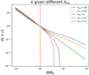 |
Fig. 1. Illustration of the transformed power-law profile in the mean dimensionless enclosed projected mass distribution under the internal MST with θs = 10″. All the transformed mass profiles share the same Einstein radius (red dashed line). All the mass distributions in this figure produce essentially the same model images (i.e., the difference of the χ2 is less than 0.001%) but a different unlensed size of the source, which is not directly observable. |
The Einstein radius of the lens system, θE, is defined as the angular radius for which  .
.
Thus, the general MST accounting for both κext and λint can be written as

where κtrue represents the true projected mass profile. In this paper we set the stage for future investigations by dissecting where the constraining power on the distance measurements in TDC comes from and exploring what assumptions have to be made and data have to be used to break the internal MST.
3. Measurement of DΔt under the MST
Once the time delays between multiple images are observed, we can measure the time-delay distance via
where c is the speed of light and θ, β, and ϕ(θ) are the image coordinates, source coordinates, and Fermat potential, respectively. The form of Eq. (8) allows the inference of the cosmological information contained in DΔt without any need for cosmological priors on the lens modeling.
However, in the presence of a MST, given the same time delays and imaging data, the transformed projected mass profile produces a different time-delay distance via

Thus, additional information is required to constrain both the internal and external MST, and thus to obtain unbiased DΔt measurements.
4. Measurement of Dd under the MST
Once the velocity dispersion of the lensing galaxy is measured, we can use high-resolution imaging of the lens system to measure the ratio Ds/Dds via
where  is the predicted line-of-sight luminosity-weighted velocity dispersion that is predicted by the mass distribution in the lensing galaxy. In this equation, J contains the angular-dependent information including the parameters describing the 3D deprojected mass distribution, ηlens, surface-brightness distribution in the lensing galaxy, ηlight, and stellar orbital anisotropy distribution, βani. In a similar way to the time-delay distance, the separability in Eq. (10) allows us to infer the cosmological distance ratio Ds/Dds without the need of cosmological priors on J. Since DΔt ∝ Dd(Ds/Dds), we can use the combination of the DΔt measurement from the time delays and Ds/Dds from velocity dispersion to obtain Dd. We discuss the effect of κext and λint on the Dd measurement in the following two sections.
4.1. External MST only
Jee et al. (2015) find that Dd is an invariant quantity under an external MST. This is because κext only contributes to the change of the normalization of 3D mass profile and does not affect its overall shape given any mass model (Suyu et al. 2013; Chen et al. 2019). That is, the predicted velocity dispersion in Eq. (10) changes to
where the minus sign means that we need to remove the mass contributed from the environment (i.e., the mass along the line of sight) inside the Einstein radius to obtain the mass of the lensing galaxy.
In order for the predicted velocity dispersion to match the observed value, Ds/Dds must transform under an external MST via
Then the time-delay distance changes via
Thus, by combining Eqs. (1), (12), and (13), we can show that Dd is invariant under the external MST,

4.2. Internal MST plus external MST
Since the velocity dispersion depends on the enclosed 3D mass of the lensing galaxy, whose shape is not conserved under an internal MST, the constraint on the Ds/Dds ratio is not mathematically scaled by  under an internal MST. We therefore must expand the Eq. (11) by including λint in the J term,
since J contains the 3D deprojected dimensionless mass model components, whose structure is affected by the value of λint. Thus, Dd can be expressed as
Many previous investigations (e.g., Suyu et al. 2014; Paper IV) show that the internal MST can be broken with a single-aperture velocity dispersion, given a cosmological model. This can be explained as follows: Firstly, the Einstein ring radius, as defined in terms of the mean dimensionless enclosed projected mass distribution ( ), is invariant under an internal MST (i.e.,
  ; see also Fig. 1), while the physical mass inside the Einstein radius is unconstrained without assuming a cosmological model. Secondly, from Eq. (15) we show hereafter that if a cosmological model is not assumed, then the values of λint and Ds/Dds, which affect the shape and normalization respectively, are degenerate. Hence, even with a measured velocity dispersion, the mass inside the effective radius is also not constrained. Therefore, a single-aperture velocity dispersion is insufficient to break the degeneracy and constrain the internal MST if we do not assume a cosmological model. Spatially resolved kinematics of the lensing galaxy would be required (Yildirim et al., in prep.).
In order to illustrate these dependences, we use the power-law mass model, which was obtained by fitting to the real imaging data of a four-image gravitational lens system (J0924+0219) shown in Fig. 2 (see Chen et al., in prep. for details), and analysed this model in the context of an internal MST (i.e., added to our model a MST component as described in Eq. (5)). For the anisotropy component, we assume βani varies with radius and parameterize this behavior in the form of an anisotropy radius, rani, in the Osipkov-Merritt formulation (Osipkov 1979; Merritt 1985),
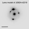 |
Fig. 2. Multiple lensed images and extended arc around the lensing galaxy from the background AGN and its reconstructed host galaxy. The foreground main lens is located in the center of the lens system. The solid horizontal line represents 1″ scale. The detailed lens modeling will be presented in Chen et al. (in prep.). The study of this paper is not limited to any specific configuration of the lens systems. |
as an example. In this formulation, rani = 0 indicates pure radial orbits and rani → ∞ is isotropic with equal radial and tangential velocity dispersions. In our models, we use a scaled version of the anisotropy parameter, aani ≡ rani/reff, where reff = Ddθeff, and θeff is the effective radius. The redshift of the lens and source are zd = 0.393 and zs = 1.523, respectively. We note that the study of this work is not limited to any specific configuration of the lens systems. We set mock time delays (ΔtAB = 10 ± 1.5 days, ΔtCB = 15 ± 1.5 days, ΔtDB = 10 ± 1.5 days) and a mock velocity dispersion measurement (= 279 ± 15 km s−1) for the analysis. The values of mock time delays and the velocity dispersion were chosen to be roughly consistent with the model of J0924 so that they would represent a physically plausible lens. Specifically, given the mass model from the J0924+0219 lens imaging, the mock time delay and velocity dispersion are created by assuming Flat ΛCDM with fixed Ωm = 0.3, H0 = 70 km s−1 Mpc−1, and λint = 1 (i.e., no internal MST). The uncertainties on the time delays and velocity dispersion are typical of time-delay lens systems. We note that all the figures produced in this work are based on this single lens. Since κext does not affect the Dd measurement and is well understood, we set κext = 0 throughout the paper for simplicity.
We consider two situations: one with a flat ΛCDM cosmology and another in which we only use the velocity dispersion, time delays, and imaging data without assuming any cosmological model. We note that throughout the paper, for flat ΛCDM cosmology, we assume Ωm = [0.05, 1.0], ΩΛ = 1 − Ωm, and H0 uniform in [0,150] km s−1 Mpc−1. The results are shown in Fig. 3, where the ΛCDM results are shown as points that are color coded by the velocity dispersion to demonstrate the link between σv and the other parameters. Figure 3 clearly demonstrates that λint can be constrained only when ΛCDM is assumed, on the contrary, when the cosmological model constraint is relaxed, Dd changes very little within the physically allowed values of λint. Thus the J term in Eq. (15) can be very well approximated as J(λint) = λintJ with < 1% shift on the distance measurement of Dd for θs = 10″ and with single aperture averaged velocity dispersion. This approximation was also used by Paper IV.
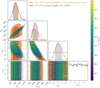 |
Fig. 3. Comparison of the Dd, DΔt, λint, and aani measurements with and without the assumption of the ΛCDM model from single time-delay mock lens. The abbreviation “TD” represents time-delay information and “VD” represents velocity dispersion information. When ΛCDM model is not assumed, the internal MST (λint) is not constrained. When ΛCDM model is assumed, the degeneracy can be broken and hence DΔt is constrained. The anisotropy parameter is not constrained in either case. Color-coded velocity dispersion shows that DΔt is positively correlated with Dd but anticorrelated with σv. The contours represent the 68.3% (shaded region) and 95.4% quantiles. |
5. Error propagation in MST
5.1. Error propagation without assuming a cosmological model
In the previous section, we showed that DΔt is directly affected by both external and internal MST, while Dd is not affected by κext and is nearly invariant. Thus, based on Eq. (9) the error on DΔt (δDΔt) given λ and λint scales as
while based on Eq. (16), the error of Dd scales as
where σv is the measured line-of-sight velocity dispersion. Thus, the uncertainties on Dd are dominated by the velocity dispersion measurement errors, while the DΔt uncertainties are dominated by both internal and external MST. Therefore, H0 inferred solely from Dd is robust against the MST (Jee et al. 2019)2.
5.2. Error propagation under ΛCDM model
However, if one assumes a ΛCDM model, the error on λint is written as

By combining Eqs. (18)–(20), the correlations between the errors on DΔt, Dd, and σv are given by
In Fig. 3, we see that under the assumption of the ΛCDM model, DΔt is positively correlated with Dd but anticorrelated with σv.
Most importantly, while Eqs. (20) and (21) tell us that DΔt and Dd are anticorrelated with λint under ΛCDM model, Dd is nearly uncorrelated with λint without assuming a cosmological model inside the physically allowed range of λint.
6. Constraining the internal MST
In the previous sections of this paper, we have shown that in the presence of an internal MST, parameterized by λint, the time-delay distance measurement is poorly constrained unless a specific cosmological model is picked. This situation is clearly demonstrated in the λint versus DΔt panel in Fig. 3, where λint is essentially unconstrained without the assumption of a cosmological model. In turn, the large uncertainties in λint translate into imprecise inferences on DΔt. Therefore, in this section we describe two approaches to improving the constraints on λint. The first approach constrains λint in a fashion that depends on the cosmological model (Paper IV), while the second approach works even if we are agnostic about the cosmological model. In both cases, we assume that observations have provided measurements of time delays and luminosity-weighted stellar velocity dispersions with errors that are typical of those found in previous works in this field.
6.1. Method 1: Choosing a cosmological model
In Sect. 4.2, we demonstrated that Ds/Dds and λint are degenerate quantities. However, once a cosmological model is assumed, Ds/Dds can be determined up to a range depending on the other cosmological parameters such as Ωm and Ωk (Grillo et al. 2008), since the unknown factor of H0 cancels out in the ratio. This means that the measurement of the velocity dispersion constrains λint, hence the mass inside the effective radius of the lensing galaxy. Once λint is constrained, DΔt is constrained and Dd can be inferred from DΔt. Hence the mass inside the Einstein radius is assigned. Therefore, by assuming a cosmological model, the internal MST can be broken to a level that depends on the precision of the velocity dispersion measurement. To further illustrate the effect of assuming a cosmological model, we show the constraining power on Dd, DΔt, λint, and the anisotropy parameter (aani) when setting the cosmological model to ΛCDM in Fig. 3. We clearly see the correlation between DΔt and inferred Dd under the assumption of the ΛCDM.
For the case in which no cosmological model is used in Fig. 3, we see that DΔt is degenerate with λint. In contrast, by assuming a cosmological model, we restrict the allowed range of λint and this places stronger constraints on the inferences on the cosmological distances. We can decompose the black contour in Fig. 3 into separate cases to examine the constraining power from the velocity dispersion only (VD only), time-delay measurements only (TD only), and a joint constraint from both measurements (VD plus TD). Figure 4 clearly shows that the velocity dispersion constrains λint when assuming a cosmological model (e.g., ΛCDM). In other words, the value of λint depends on the cosmological model and the measurement of DΔt in this case is not a cosmological model-independent quantity.
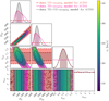 |
Fig. 4. Decomposition of the constraining power from time delays (TD), velocity dispersion (VD), and imaging data under the assumption of the ΛCDM model. When only “TD+imaging” is used, the values of Dd and DΔt are not constrained, and both of them are fully degenerate with λint. Since the velocity dispersion constrains the λint, the joint constraint (“TD+VD+imaging data”) breaks the degeneracy and hence constrains DΔt and Dd. The anisotropy parameters are not constrained in all cases. |
6.2. Method 2: Using external datasets to constrain Ds/Dds
To break the internal MST without assuming a particular cosmological model (e.g., ΛCDM model), we require additional information to constrain Ds/Dds. This can be done by including data on SN1a and BAO). The SN1a data are given as measurements of the distance modulus

where m is the apparent magnitude, M is a fiducial absolute magnitude, and DL is the luminosity distance. When M is a free parameter without calibration, SN1a only constrain the shape of the expansion history. The BAO data provide measurements of DV/rs, the dilation scale normalized by the standard ruler length (or DA/rs and Hrs in the anisotropic analysis), where
![$$ \begin{aligned} D_{V}\equiv \left[ D_{M}^{2}(z)\frac{cz}{H(z)}\right]^{1/3}, \end{aligned} $$](/articles/aa/full_html/2021/08/aa39895-20/aa39895-20-eq31.gif)
DM = (1 + z)DA, and DA is the angular diameter distance. If we vary M and rs freely, those data sets provide the information on the shape of the expansion history (e.g., Cuesta et al. 2015) and thus Ds/Dds.
However, we still require a model for the redshift distance relationship to connect these data. In this work, we choose piecewise natural cubic splines3 to describe H(z) that fit to the data. The spline method has been used in many studies to reconstruct the expansion history (Bernal et al. 2016, 2019; Poulin et al. 2018; Aylor et al. 2019). The splines are set by the values they take at different redshifts. These values can uniquely define the piecewise cubic spline once we require continuity of H(z) and its first and second derivatives at the knots, and set two boundary conditions. We also require the second derivative to vanish at the exterior knots. We set the minimal assumptions of this work: (1) cosmological principle of homogeneity and isotropy (i.e., Friedmann-Lemaître-Robertson-Walker metric); (2) assumption of general relativity: the curvature density parameter is given by Ωk = k[c/(R0H0)]2 where k = {1, 0, −1}, R0 denotes the present value of the scale factor; (3) spline H(z) completely specifies the FLRW metric; and (4) cosmic distance duality relation: DL = DA(1 + z)2.
To get a good constraint on the cosmological model-independent Ds/Dds at the redshift of the mock lens, we need the data that cover the redshift up to the source redshift4 (zs = 1.523 in this case). Current existing data show that we can constrain the shape of the expansion history up to ∼z = 2.5 (see Fig. 3 in Bernal et al. 2019). Therefore, we update the likelihood used in Bernal et al. (2019) and use the Pantheon datasets of SN1a (Scolnic et al. 2018), BAO from galaxies (Kazin et al. 2014; Alam et al. 2017; Gil-Marín et al. 2020), quasars (Hou et al. 2021; Neveux et al. 2020), and the Lyman-α forest (du Mas des Bourboux et al. 2020). For the eBOSS likelihoods, we use the Gaussian approximation and that BAO can be used to apply cosmological models beyond LCDM (Bernal et al. 2020; Carter et al. 2020). We summarize the BAO measurements and the redshift information in Table 1. We set five “knots” at different redshifts (z0 = 0, z1 = 0.25, z2 = 0.5, z3 = 1., z4 = 2.5). The complete set of parameters for the Spline model is {H0, H1, H2, H3, H4, rs, Ωk, M}. Uniform priors are assumed for all parameters. We show the reconstructed E(z)( = H(z)/H0) normalised by the values for our fiducial cosmology given by the best-fitting parameters from the Planck analysis for a ΛCDM model in Fig. 5. The posterior of Ds/Dds can be obtained by integrating E(z).
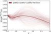 |
Fig. 5. Results of the reconstruction of E(z) (=H(z)/H0) using the SN1a and BAO data, normalized by the values for our fiducial cosmology given by the best-fitting parameters from the Planck analysis for a ΛCDM model. Each thin line comes from a random draw among the points in parameter space within 68% confidence level. The thick line in the middle represents the best fit. The uncertainties are relatively large at z = 1 − 1.5 since the error bars of the Baryon acoustic oscillations (BAO) measurements at z = 0.8, and especially, at z = 1.5, are significantly larger, while SN1a measurements are only powerful enough to constrain the splines at z ∼ 0.8 − 1. The shape of expansion history is described by piecewise natural cubic splines. The splines constrained by the data can be used to constrain Ds/Dds and hence break the internal MST. |
Summary of the BAO measurements that are used in this work.
In Fig. 6, we show that by combining the inference from the external datasets on H(z)/H0, which constrain Ds/Dds, with time-delay strong lensing systems, we can obtain cosmological model-independent Dd and DΔt measurements that are comparable to those obtained by assuming a ΛCDM or wCDM cosmology. In addition, we also see that the values of λint under ΛCDM and wCDM are slightly offset from the cases that include SN1a and BAO datasets. This is because the flat priors on Ωm and w in ΛCDM and wCDM models do not reflect the expansion history described by the SN1a and BAO datasets. Thus, it indicates the importance of including the external datasets, which directly constrain the expansion history to get distance measurements.
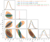 |
Fig. 6. Comparison of the inferred Dd, Ds/Dds, DΔt, and λint in different cases. Case 1 (orange): The distance measurements directly from single time-delay mock lens without assuming any cosmological model. Case 2 (blue): The distance measurements under the assumption of the flat wCDM model with Ωm = [0.05, 1.0], Ωde = 1 − Ωm, w = [ − 2.5, 0.5], and H0 uniform in [0,150] km s−1 Mpc−1. Case 3 (black): The distance measurements under the assumption of the ΛCDM model with Ωm = [0.05, 1.0], ΩΛ = 1 − Ωm, and H0 uniform in [0,150] km s−1 Mpc−1 Case 4: (green): The distance measurements from single time-delay mock lens, Pantheon dataset, and BAO dataset by using splines with free Ωk. Case 5 (red): The distance measurements from single time-delay mock lens, Pantheon dataset, and BAO dataset by using splines with Ωk = 0. For the cases (green and red) that do not assume a particular cosmological model, the constraining power on λint is comparable to the cases (blue and black) with an assumption of having a underlying cosmological model. |
In Fig. 7, we show the distance measurements from combining a single time-delay lens with SN1a and BAO with free Ωk (the green contour in Fig. 6). This distance measurements can be used to infer H0 in generic cosmological models. We emphasize that this approach does not require the absolute calibration of SN1a or BAO; thus, the derived constraint on H0 remains independent of the distance ladder and the sound horizon scale.
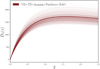 |
Fig. 7. Cosmological model-independent distance measurements from combining single time-delay mock lens with Pantheon and BAO datasets. Each thin line comes from a random draw among the points in parameter space within 68% confidence level. The thick line in the middle represents the best fit. |
6.3. Comparison with Paper IV
In the previous section, we demonstrate that Ds/Dds is fully degenerate with λint, which affects the time-delay distance measurement. Therefore, we compare the redshift-dependent median value of Ds/Dds, constrained directly by the SN and BAO data at the redshift of the current seven TDCOSMO lens samples, with the Ds/Dds in Paper IV, which used the prior based on Pantheon sample with Ωm = 0.298 ± 0.022 (Scolnic et al. 2018) under the assumption of the ΛCDM model. These results shown in Fig. 8 demonstrate that in the case of these seven lenses, using the prior information from Pantheon datasets that constrain the low redshift expansion history and then using ΛCDM model to extrapolate the constraint on Ds/Dds to high redshift are valid approaches, becausethe deviations from the median value of Ds/Dds are all below 1%, thereby demonstrating that the shape of the expansion history is described well by the ΛCDM model. However, the time-delay distance measurements derived by the method developed in this work are broadly applicable distance posteriors, which can be used to infer H0 in various cosmological models.
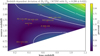 |
Fig. 8. Percent difference between the median value of Ds/Dds, directly constrained from the SN1a and BAO, and the Ds/Dds under the assumption of the ΛCDM model with Ωm = 0.298 ± 0.022 (Scolnic et al. 2018), which was used in Paper IV. All 7 time-delay lenses show < 1% deviation validate the use of the Pantheon datasets that constrain the low-redshift expansion history and the use of ΛCDM model that extrapolates the constraint on Ds/Dds at high redshift. |
7. Conclusions
In this work, we use a mock gravitational lens system to study the correlation between distance measurements under the MST with or without assuming a cosmological model. We verify that although DΔt is directly correlated with both the internal and external MST, Dd is not only invariant under an external MST but is also insensitive to the internal MST. Thus, without assuming any particular cosmological model, the role of velocity dispersion is to obtain the angular diameter distance to the lens (Dd) rather than break the internal MST (λint). To break λint, in addition to the velocity dispersion, we identify that constraining Ds/Dds is the key, which is typically achieved through the assumption of a particular cosmological model, and hence λint and DΔt are both cosmological-model-dependent quantities. In this work, we show that cosmological model-independent DΔt measurement can be achieved when relative distance indicators (e.g., SN1a and BAO) are used to constrain Ds/Dds and hence λint. These distance measurements with SN1a and BAO shown in Fig. 7 can then be used to infer H0 in generic cosmological models. It is important to stress that this approach does not require the absolute calibration of SN1a or BAO; thus, the derived constraint on H0 remains independent5 of the distance ladder and the sound horizon scale.
We note that Jee et al. (2019) shows that different anisotropy model may slightly shift the inferred Dd value.
We note that linear interpolation (e.g., Verde et al. 2017), Gaussian processes (e.g., Joudaki et al. 2018; Liao et al. 2020), or smooth Taylor expansion (e.g., Macaulay et al. 2019; Wojtak & Agnello 2019; Arendse et al. 2020) are alternatives.
Acknowledgments
GC-FC thanks Simon Birrer, Adriano Agnello, James Chan, Tommaso Treu, Dominique Sluse, Matt Auger, and Elizabeth Buckley-Geer for many insightful comments. GC-FC thanks Alessandro Sonnenfeld for useful suggestions on using stellar kinematics code and Ken Wong for the code review. GC-FC acknowledges support by NSF through grants NSF-AST-1906976 and NSF-AST-1836016. GC-FC acknowledges support from the Moore Foundation through grant 8548. GC-FC and CDF acknowledge support for this work from the National Science Foundation under Grant Nos. AST-171561 and AST-1907396. SHS and AY thank the Max Planck Society for support through the Max Planck Research Group for SHS. SHS and EK are supported in part by the Deutsche Forschungsgemeinschaft (DFG, German Research Foundation) under Germany’s Excellence Strategy – EXC-2094 – 390783311. The Kavli IPMU is supported by World Premier International Research Center Initiative (WPI), MEXT, Japan. J. L. B. is supported by the Allan C. and Dorothy H. Davis Fellowship.
References
- Alam, S., Ata, M., Bailey, S., et al. 2017, MNRAS, 470, 2617 [NASA ADS] [CrossRef] [Google Scholar]
- Arendse, N., Wojtak, R. J., Agnello, A., et al. 2020, A&A, 639, A57 [EDP Sciences] [Google Scholar]
- Auger, M. W., Treu, T., Bolton, A. S., et al. 2010, ApJ, 724, 511 [Google Scholar]
- Aylor, K., Joy, M., Knox, L., et al. 2019, ApJ, 874, 4 [NASA ADS] [CrossRef] [Google Scholar]
- Barkana, R. 1998, ApJ, 502, 531 [Google Scholar]
- Barnabè, M., Czoske, O., Koopmans, L. V. E., Treu, T., & Bolton, A. S. 2011, MNRAS, 415, 2215 [NASA ADS] [CrossRef] [Google Scholar]
- Bernal, J. L., Verde, L., & Riess, A. G. 2016, JCAP, 10, 019 [NASA ADS] [CrossRef] [Google Scholar]
- Bernal, J. L., Breysse, P. C., & Kovetz, E. D. 2019, Phys. Rev. Lett., 123, 251301 [CrossRef] [Google Scholar]
- Bernal, J. L., Smith, T. L., Boddy, K. K., & Kamionkowski, M. 2020, Phys. Rev. D, 102, 123515 [CrossRef] [Google Scholar]
- Beutler, F., Blake, C., Colless, M., et al. 2011, MNRAS, 416, 3017 [Google Scholar]
- Birrer, S., Treu, T., Rusu, C. E., et al. 2019, MNRAS, 484, 4726 [NASA ADS] [CrossRef] [Google Scholar]
- Birrer, S., Shajib, A. J., Galan, A., et al. 2020, A&A, 643, A165 [CrossRef] [EDP Sciences] [Google Scholar]
- Blum, K., Castorina, E., & Simonović, M. 2020, ApJ, 892, L27 [CrossRef] [Google Scholar]
- Bolton, A. S., Burles, S., Schlegel, D. J., Eisenstein, D. J., & Brinkmann, J. 2004, AJ, 127, 1860 [NASA ADS] [CrossRef] [Google Scholar]
- Bolton, A. S., Burles, S., Koopmans, L. V. E., Treu, T., & Moustakas, L. A. 2006, ApJ, 638, 703 [Google Scholar]
- Bonvin, V., Tewes, M., Courbin, F., et al. 2016, A&A, 585, A88 [NASA ADS] [CrossRef] [EDP Sciences] [Google Scholar]
- Bonvin, V., Chan, J. H. H., Millon, M., et al. 2018, A&A, 616, A183 [NASA ADS] [CrossRef] [EDP Sciences] [Google Scholar]
- Buckley-Geer, E. J., Lin, H., Rusu, C. E., et al. 2020, MNRAS, 498, 3241 [CrossRef] [Google Scholar]
- Cappellari, M. 2016, ARA&A, 54, 597 [NASA ADS] [CrossRef] [Google Scholar]
- Carter, P., Beutler, F., Percival, W. J., et al. 2020, MNRAS, 494, 2076 [CrossRef] [Google Scholar]
- Chen, G. C. F., Fassnacht, C. D., Suyu, S. H., et al. 2019, MNRAS, 2193 [Google Scholar]
- Collett, T. E., Marshall, P. J., Auger, M. W., et al. 2013, MNRAS, 432, 679 [NASA ADS] [CrossRef] [Google Scholar]
- Cuesta, A. J., Verde, L., Riess, A., & Jimenez, R. 2015, MNRAS, 448, 3463 [NASA ADS] [CrossRef] [Google Scholar]
- du Mas des Bourboux, H., Rich, J., Font-Ribera, A., et al. 2020, ApJ, 901, 153 [Google Scholar]
- Efstathiou, G. 2020, ArXiv e-prints [arXiv:2007.10716] [Google Scholar]
- Falco, E. E., Gorenstein, M. V., & Shapiro, I. I. 1985, ApJ, 289, L1 [Google Scholar]
- Fassnacht, C. D., Xanthopoulos, E., Koopmans, L. V. E., & Rusin, D. 2002, ApJ, 581, 823 [NASA ADS] [CrossRef] [Google Scholar]
- Fassnacht, C. D., Gal, R. R., Lubin, L. M., et al. 2006, ApJ, 642, 30 [NASA ADS] [CrossRef] [Google Scholar]
- Freedman, W. L., Madore, B. F., Hatt, D., et al. 2019, ApJ, 882, 34 [Google Scholar]
- Gil-Marín, H., Bautista, J. E., Paviot, R., et al. 2020, MNRAS, 498, 2492 [Google Scholar]
- Gomer, M., & Williams, L. L. R. 2020, JCAP, 2020, 045 [CrossRef] [Google Scholar]
- Gorenstein, M. V., Falco, E. E., & Shapiro, I. I. 1988, ApJ, 327, 693 [NASA ADS] [CrossRef] [Google Scholar]
- Greene, Z. S., Suyu, S. H., Treu, T., et al. 2013, ApJ, 768, 39 [NASA ADS] [CrossRef] [Google Scholar]
- Grillo, C., Lombardi, M., & Bertin, G. 2008, A&A, 477, 397 [NASA ADS] [CrossRef] [EDP Sciences] [Google Scholar]
- Hinshaw, G., Larson, D., Komatsu, E., et al. 2013, ApJS, 208, 19 [Google Scholar]
- Hou, J., Sánchez, A. G., Ross, A. J., et al. 2021, MNRAS, 500, 1201 [Google Scholar]
- Humphrey, P. J., & Buote, D. A. 2010, MNRAS, 403, 2143 [NASA ADS] [CrossRef] [Google Scholar]
- Jee, I., Komatsu, E., & Suyu, S. H. 2015, JCAP, 11, 033 [NASA ADS] [CrossRef] [Google Scholar]
- Jee, I., Suyu, S. H., Komatsu, E., et al. 2019, Science, 365, 1134 [CrossRef] [Google Scholar]
- Joudaki, S., Kaplinghat, M., Keeley, R., & Kirkby, D. 2018, Phys. Rev. D, 97, 123501 [CrossRef] [Google Scholar]
- Kazin, E. A., Koda, J., Blake, C., et al. 2014, MNRAS, 441, 3524 [Google Scholar]
- Kochanek, C. S. 2020, MNRAS, 493, 1725 [CrossRef] [Google Scholar]
- Komatsu, E., Smith, K. M., Dunkley, J., et al. 2011, ApJS, 192, 18 [NASA ADS] [CrossRef] [Google Scholar]
- Koopmans, L. V. E., Treu, T., Bolton, A. S., Burles, S., & Moustakas, L. A. 2006, ApJ, 649, 599 [NASA ADS] [CrossRef] [Google Scholar]
- Koopmans, L. V. E., Bolton, A., Treu, T., et al. 2009, ApJ, 703, L51 [NASA ADS] [CrossRef] [Google Scholar]
- Liao, K., Shafieloo, A., Keeley, R. E., & Linder, E. V. 2020, ApJ, 895, L29 [CrossRef] [Google Scholar]
- Liesenborgs, J., de Rijcke, S., Dejonghe, H., & Bekaert, P. 2008, MNRAS, 389, 415 [NASA ADS] [CrossRef] [Google Scholar]
- Macaulay, E., Nichol, R. C., Bacon, D., et al. 2019, MNRAS, 966 [Google Scholar]
- Merritt, D. 1985, AJ, 90, 1027 [NASA ADS] [CrossRef] [Google Scholar]
- Millon, M., Galan, A., Courbin, F., et al. 2020, A&A, 639, A101 [CrossRef] [EDP Sciences] [Google Scholar]
- Navarro, J. F., Frenk, C. S., & White, S. D. M. 1996, ApJ, 462, 563 [Google Scholar]
- Neveux, R., Burtin, E., de Mattia, A., et al. 2020, MNRAS, 499, 210 [Google Scholar]
- Osipkov, L. P. 1979, Pis ma Astronomicheskii Zhurnal, 5, 77 [Google Scholar]
- Planck Collaboration VI. 2020, A&A, 641, A6 [NASA ADS] [CrossRef] [EDP Sciences] [Google Scholar]
- Poulin, V., Boddy, K. K., Bird, S., & Kamionkowski, M. 2018, Phys. Rev. D, 97, 123504 [CrossRef] [Google Scholar]
- Refsdal, S. 1964, MNRAS, 128, 307 [NASA ADS] [CrossRef] [Google Scholar]
- Riess, A. G., Casertano, S., Yuan, W., Macri, L. M., & Scolnic, D. 2019, ApJ, 876, 85 [Google Scholar]
- Ross, A. J., Samushia, L., Howlett, C., et al. 2015, MNRAS, 449, 835 [Google Scholar]
- Rusu, C. E., Fassnacht, C. D., Sluse, D., et al. 2017, MNRAS, 467, 4220 [NASA ADS] [CrossRef] [Google Scholar]
- Rusu, C. E., Wong, K. C., Bonvin, V., et al. 2019, MNRAS, 498, 1440 [CrossRef] [Google Scholar]
- Saha, P. 2000, AJ, 120, 1654 [NASA ADS] [CrossRef] [Google Scholar]
- Schneider, P., & Sluse, D. 2013, A&A, 559, A37 [NASA ADS] [CrossRef] [EDP Sciences] [Google Scholar]
- Scolnic, D. M., Jones, D. O., Rest, A., et al. 2018, ApJ, 859, 101 [Google Scholar]
- Shajib, A. J., Birrer, S., Treu, T., et al. 2020, MNRAS, 494, 6072 [Google Scholar]
- Shajib, A. J., Treu, T., Birrer, S., & Sonnenfeld, A. 2021, MNRAS, 503, 2380 [Google Scholar]
- Sonnenfeld, A., Treu, T., Gavazzi, R., et al. 2013, ApJ, 777, 98 [Google Scholar]
- Suyu, S. H., Marshall, P. J., Blandford, R. D., et al. 2009, ApJ, 691, 277 [Google Scholar]
- Suyu, S. H., Marshall, P. J., Auger, M. W., et al. 2010, ApJ, 711, 201 [NASA ADS] [CrossRef] [Google Scholar]
- Suyu, S. H., Auger, M. W., Hilbert, S., et al. 2013, ApJ, 766, 70 [NASA ADS] [CrossRef] [Google Scholar]
- Suyu, S. H., Treu, T., Hilbert, S., et al. 2014, ApJ, 788, L35 [NASA ADS] [CrossRef] [Google Scholar]
- Suyu, S. H., Chang, T.-C., Courbin, F., & Okumura, T. 2018, Space Sci. Rev., 214, 91 [NASA ADS] [CrossRef] [Google Scholar]
- Taubenberger, S., Suyu, S. H., Komatsu, E., et al. 2019, A&A, 628, L7 [NASA ADS] [CrossRef] [EDP Sciences] [Google Scholar]
- Tihhonova, O., Courbin, F., Harvey, D., et al. 2018, MNRAS, 477, 5657 [NASA ADS] [CrossRef] [Google Scholar]
- Treu, T., & Marshall, P. J. 2016, A&ARv, 24, 11 [Google Scholar]
- Verde, L., Bernal, J. L., Heavens, A. F., & Jimenez, R. 2017, MNRAS, 467, 731 [NASA ADS] [Google Scholar]
- Verde, L., Treu, T., & Riess, A. G. 2019, Nat. Astron., 3, 891 [Google Scholar]
- Wojtak, R., & Agnello, A. 2019, MNRAS, 486, 5046 [NASA ADS] [CrossRef] [Google Scholar]
- Wong, K. C., Suyu, S. H., Chen, G. C.-F., et al. 2019, MNRAS, 498, 1420 [Google Scholar]
- Xu, D., Sluse, D., Schneider, P., et al. 2016, MNRAS, 456, 739 [NASA ADS] [CrossRef] [Google Scholar]
All Tables
All Figures
|
Fig. 1. Illustration of the transformed power-law profile in the mean dimensionless enclosed projected mass distribution under the internal MST with θs = 10″. All the transformed mass profiles share the same Einstein radius (red dashed line). All the mass distributions in this figure produce essentially the same model images (i.e., the difference of the χ2 is less than 0.001%) but a different unlensed size of the source, which is not directly observable. |
| In the text | |
|
Fig. 2. Multiple lensed images and extended arc around the lensing galaxy from the background AGN and its reconstructed host galaxy. The foreground main lens is located in the center of the lens system. The solid horizontal line represents 1″ scale. The detailed lens modeling will be presented in Chen et al. (in prep.). The study of this paper is not limited to any specific configuration of the lens systems. |
| In the text | |
|
Fig. 3. Comparison of the Dd, DΔt, λint, and aani measurements with and without the assumption of the ΛCDM model from single time-delay mock lens. The abbreviation “TD” represents time-delay information and “VD” represents velocity dispersion information. When ΛCDM model is not assumed, the internal MST (λint) is not constrained. When ΛCDM model is assumed, the degeneracy can be broken and hence DΔt is constrained. The anisotropy parameter is not constrained in either case. Color-coded velocity dispersion shows that DΔt is positively correlated with Dd but anticorrelated with σv. The contours represent the 68.3% (shaded region) and 95.4% quantiles. |
| In the text | |
|
Fig. 4. Decomposition of the constraining power from time delays (TD), velocity dispersion (VD), and imaging data under the assumption of the ΛCDM model. When only “TD+imaging” is used, the values of Dd and DΔt are not constrained, and both of them are fully degenerate with λint. Since the velocity dispersion constrains the λint, the joint constraint (“TD+VD+imaging data”) breaks the degeneracy and hence constrains DΔt and Dd. The anisotropy parameters are not constrained in all cases. |
| In the text | |
|
Fig. 5. Results of the reconstruction of E(z) (=H(z)/H0) using the SN1a and BAO data, normalized by the values for our fiducial cosmology given by the best-fitting parameters from the Planck analysis for a ΛCDM model. Each thin line comes from a random draw among the points in parameter space within 68% confidence level. The thick line in the middle represents the best fit. The uncertainties are relatively large at z = 1 − 1.5 since the error bars of the Baryon acoustic oscillations (BAO) measurements at z = 0.8, and especially, at z = 1.5, are significantly larger, while SN1a measurements are only powerful enough to constrain the splines at z ∼ 0.8 − 1. The shape of expansion history is described by piecewise natural cubic splines. The splines constrained by the data can be used to constrain Ds/Dds and hence break the internal MST. |
| In the text | |
|
Fig. 6. Comparison of the inferred Dd, Ds/Dds, DΔt, and λint in different cases. Case 1 (orange): The distance measurements directly from single time-delay mock lens without assuming any cosmological model. Case 2 (blue): The distance measurements under the assumption of the flat wCDM model with Ωm = [0.05, 1.0], Ωde = 1 − Ωm, w = [ − 2.5, 0.5], and H0 uniform in [0,150] km s−1 Mpc−1. Case 3 (black): The distance measurements under the assumption of the ΛCDM model with Ωm = [0.05, 1.0], ΩΛ = 1 − Ωm, and H0 uniform in [0,150] km s−1 Mpc−1 Case 4: (green): The distance measurements from single time-delay mock lens, Pantheon dataset, and BAO dataset by using splines with free Ωk. Case 5 (red): The distance measurements from single time-delay mock lens, Pantheon dataset, and BAO dataset by using splines with Ωk = 0. For the cases (green and red) that do not assume a particular cosmological model, the constraining power on λint is comparable to the cases (blue and black) with an assumption of having a underlying cosmological model. |
| In the text | |
|
Fig. 7. Cosmological model-independent distance measurements from combining single time-delay mock lens with Pantheon and BAO datasets. Each thin line comes from a random draw among the points in parameter space within 68% confidence level. The thick line in the middle represents the best fit. |
| In the text | |
|
Fig. 8. Percent difference between the median value of Ds/Dds, directly constrained from the SN1a and BAO, and the Ds/Dds under the assumption of the ΛCDM model with Ωm = 0.298 ± 0.022 (Scolnic et al. 2018), which was used in Paper IV. All 7 time-delay lenses show < 1% deviation validate the use of the Pantheon datasets that constrain the low-redshift expansion history and the use of ΛCDM model that extrapolates the constraint on Ds/Dds at high redshift. |
| In the text | |
Current usage metrics show cumulative count of Article Views (full-text article views including HTML views, PDF and ePub downloads, according to the available data) and Abstracts Views on Vision4Press platform.
Data correspond to usage on the plateform after 2015. The current usage metrics is available 48-96 hours after online publication and is updated daily on week days.
Initial download of the metrics may take a while.