| Issue |
A&A
Volume 652, August 2021
|
|
|---|---|---|
| Article Number | A136 | |
| Number of page(s) | 21 | |
| Section | Extragalactic astronomy | |
| DOI | https://doi.org/10.1051/0004-6361/202039137 | |
| Published online | 24 August 2021 | |
SN 2020bqj: A Type Ibn supernova with a long-lasting peak plateau⋆
1
The Oskar Klein Centre, Department of Astronomy, Stockholm University, AlbaNova, 10691 Stockholm, Sweden
e-mail: This email address is being protected from spambots. You need JavaScript enabled to view it.
2
Department of Physics and Astronomy, Aarhus University, Ny Munkegade 120, 8000 Aarhus C, Denmark
3
Department of Particle Physics and Astrophysics, Weizmann Institute of Science, Rehovot 7610001, Israel
4
Tuorla Observatory, Department of Physics and Astronomy, University of Turku, 20014 Turku, Finland
5
DiRAC Institute, Department of Astronomy, University of Washington, 3910 15th Avenue NE, Seattle, WA 98195, USA
6
Cahill Center for Astrophysics, California Institute of Technology, 1200 E. California Blvd., Pasadena, CA 91125, USA
7
Division of Physics, Mathematics, and Astronomy, California Institute of Technology, Pasadena, CA 91125, USA
8
The eScience Institute, University of Washington, Seattle, WA 98195, USA
9
Astrophysics Group, Cavendish Laboratory, 19 J. J. Thomson Avenue, Cambridge CB3 0HE, UK
10
Racah Institute of Physics, The Hebrew University of Jerusalem, Jerusalem 91904, Israel
11
Caltech Optical Observatories, California Institute of Technology, Pasadena, CA 91125, USA
12
Université de Lyon, Université Claude Bernard Lyon 1, CNRS/IN2P3, IP2I Lyon, 69622 Villeurbanne, France
13
IPAC, California Institute of Technology, 1200 E. California Blvd., Pasadena, CA 91125, USA
14
Institute of Physics, Humboldt-Universität zu Berlin, Newtonstr. 15, 12489 Berlin, Germany
15
Astrophysics Research Institute, Liverpool John Moores University, 146 Brownlow Hill, Liverpool L3 5RF, UK
16
Theoretical Astrophysics, 350-17 California Institute of Technology, Pasadena, CA 91125, USA
17
Lawrence Berkeley National Laboratory, 1 Cyclotron Road, Berkeley, CA 94720, USA
18
Jodrell Bank Centre for Astrophysics, School of Physics and Astronomy, The University of Manchester, Manchester M13 9PL, UK
Received:
10
August
2020
Accepted:
26
February
2021
Abstract
Context. Type Ibn supernovae (SNe Ibn) are a rare class of stripped envelope supernovae interacting with a helium-rich circumstellar medium (CSM). The majority of the SNe Ibn reported in the literature display a surprising homogeneity in their fast-evolving lightcurves and are typically found in actively starforming spiral galaxies.
Aims. We present the discovery and the study of SN 2020bqj (ZTF20aalrqbu), a SN Ibn with a long-duration peak plateau lasting 40 days and hosted by a faint low-mass galaxy. We aim to explain its peculiar properties using an extensive photometric and spectroscopic data set.
Methods. We compare the photometric and spectral evolution of SN 2020bqj with regular SNe Ibn from the literature, as well as with other outliers in the SN Ibn subclass. We fit the bolometric and multi-band lightcurves with powering mechanism models such as radioactive decay and CSM interaction. We also model the host galaxy of SN 2020bqj.
Results. The risetime, peak magnitude and spectral features of SN 2020bqj are consistent with those of most SNe Ibn, but the SN is a clear outlier in the subclass based on its bright, long-lasting peak plateau and the low mass of its faint host galaxy. We show through modeling that the lightcurve of SN 2020bqj can be powered predominantly by shock heating from the interaction of the SN ejecta and a dense CSM, combined with radioactive decay. The peculiar Type Ibn SN 2011hw is a close analog to SN 2020bqj in terms of lightcurve and spectral evolution, suggesting a similar progenitor and CSM scenario. In this scenario a very massive progenitor star in the transitional phase between a luminous blue variable and a compact Wolf-Rayet star undergoes core-collapse, embedded in a dense helium-rich CSM with an elevated opacity compared to normal SNe Ibn, due to the presence of residual hydrogen. This scenario is consistent with the observed properties of SN 2020bqj and the modeling results.
Conclusions. SN 2020bqj is a compelling example of a transitional SN Ibn/IIn based on not only its spectral features, but also its lightcurve, host galaxy properties and the inferred progenitor properties. The strong similarity with SN 2011hw suggests this subclass may be the result of a progenitor in a stellar evolution phase that is distinct from those of progenitors of regular SNe Ibn.
Key words: supernovae: general / supernovae: individual: SN 2020bqj / supernovae: individual: SN 2011hw
Spectra are available on WISeREP: https://www.wiserep.org/object/14231. Full Table A.1 is only available at the CDS via anonymous ftp to cdsarc.u-strasbg.fr (130.79.128.5) or via http://cdsarc.u-strasbg.fr/viz-bin/cat/J/A+A/652/A136
© ESO 2021
1. Introduction
Supernovae of Type Ibn (SNe Ibn) are a rare class of core-collapse SNe, with less than 40 objects reported in the literature (Hosseinzadeh et al. 2019). SNe Ibn are classified based on spectra that are dominated by relatively narrow (∼few × 103 km s−1, hence the ‘n’ suffix) helium (He) emission lines while showing little to no hydrogen (H). The intermediate-width emission lines are interpreted as a sign of shock interaction between the fast-moving SN ejecta and a slow-moving He-rich, but H-depleted, circumstellar medium (CSM; for a review see Smith 2017). The He-rich CSM around SNe Ibn is assumed to have originated from their progenitor stars through mass-loss, as is known to be the case for their Type IIn SN counterparts (SNe with spectra showing narrow H emission lines) based on observations of pre-SN outbursts (Fraser et al. 2013; Ofek et al. 2013, 2014; Strotjohann et al. 2021). As such, SNe Ibn are expected to be stripped-envelope SNe (SE SNe) embedded in a He-rich environment (Pastorello et al. 2008a; Foley et al. 2007; Chugai 2009).
Based on the He-rich CSM around SNe Ibn, with unperturbed CSM velocities of ∼500−1500 km s−1 (Pastorello et al. 2016), the progenitors of SNe Ibn are commonly assumed to be massive evolved Wolf-Rayet (WR) stars, which have atmospheres that are nearly H-free and exhibit mass-loss through strong and fast winds (Prinja et al. 1990; Crowther 2007). Furthermore, virtually all SNe Ibn are observed to occur in star-forming galaxies (Pastorello et al. 2015a), supporting the association of SNe Ibn to short-lived massive progenitors such as WR stars.
In so-called interacting SNe such as SNe Ibn, the shock interaction between ejecta and CSM converts kinetic energy to visible light, which means CSM interaction contributes to (or even dominates) the observed energy output of an interacting SN. In Type IIn SNe this results in a large diversity in lightcurves (e.g., Taddia et al. 2013; Nyholm et al. 2020), due to variation in the properties (composition, density, mass, geometry) of the CSM (Smith 2017; Soumagnac et al. 2019). In contrast, the lightcurves of SNe Ibn are surprisingly homogeneous. They are typically fast and evolve monotonically with a risetime of ≲15 days to a peak absolute magnitude of Mr ≈ −19, followed by a decline at a rate of ∼0.05−0.15 mag day−1 during the first month after peak (Hosseinzadeh et al. 2017). Normal SE SNe (Type Ib/c) have lightcurves that are generally consistent with powering by the decay of radioactive material synthesized in the explosion and present in the ejecta (56Ni → 56Co → 56Fe, e.g., Prentice et al. 2016). In the case of SNe Ibn, however, the high peak luminosity and the rapid lightcurve evolution typically exclude 56Ni decay as the main powering mechanism for their lightcurves, as the decline rate is usually too steep to reconcile with the amount of 56Ni required to explain the peak luminosity (e.g., Moriya & Maeda 2016). Instead, models combining radioactive decay and interaction with a (He-rich) CSM shell have been used to reproduce the observed fast-evolving SN Ibn lightcurves (Karamehmetoglu et al. 2021; Wang & Li 2020; Clark et al. 2020; Gangopadhyay et al. 2020). These model fits result in 56Ni and CSM masses that are consistent with WR progenitors, although they are affected by substantial uncertainties and degeneracy given the large number of free model parameters.
Despite the apparent match of the massive WR progenitor scenario with observed SN Ibn properties, there are still many open questions regarding the conditions and origin of the CSM, the homogeneity of SN Ibn progenitors, and the (dominant) powering mechanisms of SNe Ibn. Unlike Type IIn SNe where some have been linked to H-rich luminous blue variable (LBV) stars (e.g., Gal-Yam et al. 2007; Trundle et al. 2008; Gal-Yam & Leonard 2009; Smith et al. 2010), there have been no direct progenitor detections of SNe Ibn. The only direct evidence of a massive SN Ibn progenitor has been a luminous outburst of the prototypical Type Ibn SN 2006jc, observed two years before explosion (Nakano et al. 2006). In contrast with LBV stars, such eruptions are not common for H-deficient WR stars, so the precursor of SN 2006jc was deemed to have been a massive star with residual LBV-like properties (Foley et al. 2007; Pastorello et al. 2007), which would also explain the presence of faint H emission in the spectra. The outburst is assumed to be the source of the He-rich CSM shell, rather than a steady WR wind, based on the temporal coincidence of the outburst and the SN, and the high mass-loss rate inferred from the distance and mass of the CSM (Anupama et al. 2009; Sun et al. 2020).
An alternative scenario for the outburst preceding SN 2006jc involves an LBV companion in a binary system with the progenitor of SN 2006jc (Pastorello et al. 2007, 2008a). In fact, there is evidence of a surviving binary companion at the position of SN 2006jc (Maund et al. 2016), but the composition of the CSM and the properties of the surviving companion do not appear consistent with an LBV star (Sun et al. 2020). However, the detection of a potential binary companion at the position of SN 2006jc does suggest an alternative progenitor channel for SNe Ibn. The binary channel allows the progenitor to be of lower mass, stripped from its H envelope through binary interaction, rather than through mass-loss by a massive progenitor. Such an older low-mass progenitor could also explain PS1-12sk, the only SN Ibn known so far that was located at a site with extremely limited local star formation (SF; Hosseinzadeh et al. 2019), in an elliptical cluster galaxy (Sanders et al. 2013).
Finally, there are a few examples of SNe Ibn with lightcurves that do not fit well the SN Ibn lightcurve template from Hosseinzadeh et al. (2017), either by showing multiple peaks or a slower evolution. In the case of SN 2011hw, a scenario of a progenitor transitioning between the LBV and WR phases has been suggested to explain its spectral features (such as Balmer emission), and its unusual long-lived lightcurve (Smith et al. 2012; Pastorello et al. 2015b). SN 2011hw represents a small subset of SNe Ibn with H in their spectra and atypical lightcurves that are classified as transitional Type Ibn/IIn SNe (Pastorello et al. 2015b). However, the slowly evolving SN Ibn OGLE-2014-SN-131 did not show strong Balmer lines (Karamehmetoglu et al. 2017), and there are numerous examples of ‘normal’ fast-evolving SNe Ibn with (prominent) H in their spectra (e.g., Pastorello et al. 2015a; Karamehmetoglu et al. 2021).
In this paper we report on the discovery and the extensive follow-up program of SN 2020bqj, an outlier in the SN Ibn subclass in almost all aspects. SN 2020bqj reached a peak magnitude of Mr ∼ −19.3 in less than six days, which is consistent with the subclass, but instead of declining afterwards the SN stayed roughly constant in magnitude for ∼40 days, followed by a slow linear decline spanning > 90 days. Additionally, in contrast to normal SNe Ibn, SN 2020bqj was not located in a star-forming spiral galaxy, but instead the host appears to be a faint low-mass galaxy. Finally, the spectrum of SN 2020bqj shows, in addition to intermediate-width He in emission, prominent C II emission lines during the first half of its lightcurve, while at later epochs Hα, O I, Mg II and Ca II gain prominence.
This paper is organized as follows: In Sect. 2 the observations of SN 2020bqj are described. Sections 3–5 include analyses of the lightcurve, the spectrum and the host galaxy properties, respectively, where we compare these properties to those of SNe Ibn from the literature. In Sect. 6 we investigate the powering mechanisms of SN 2020bqj by fitting models to the lightcurve. In Sect. 7 we discuss the implications of our analysis of SN 2020bqj on its CSM composition and SN progenitor properties. Finally, in Sect. 8 we summarize our findings. Throughout this paper we adopt a flat cosmology with H0 = 70 km s−1 Mpc−1 and ΩM = 0.3.
2. Observations
2.1. Discovery
SN 2020bqj (=ZTF20aalrqbu), located at RA = 15h 33m
 and Dec = +34° 28′
  (J2000.0), was first detected by the Zwicky Transient Facility (ZTF; Bellm et al. 2019a; Graham et al. 2019) with the ZTF camera (Dekany et al. 2020) mounted on the Palomar 48 inch (P48) telescope on 2020 February 2 (MJD 58881.52) with host subtracted AB magnitudes of g = 18.05 ± 0.06 and r = 18.41 ± 0.06 (all magnitudes in this work are given in the AB system). The transient was discovered in the ZTF alert stream (Patterson et al. 2019) after passing a filter that searches for fast rising transients, and subsequent monitoring was coordinated through the GROWTH Marshal (Kasliwal et al. 2019). The transient was reported to the Transient Name Server (TNS) on the same day (Nordin et al. 2020), and based on a spectrum obtained with the SPectrograph for the Rapid Acquisition of Transients (SPRAT; Piascik et al. 2014) on the Liverpool Telescope (LT; Steele 2004), it was classified as a Type Ibn SN on 2020 February 21 (Perley et al. 2020). Previous to discovery the field was last observed by ZTF in g- and r-band 3.0 days before, where the SN was not detected with global upper limits of g > 20.2 mag and r > 20.0 mag.
SN 2020bqj appears hostless in our optical images, see Fig. 1, but a faint source (r ∼ 23.5) is reported in the eighth data release of the Dark Energy Spectroscopic Instrument (DESI) Legacy Survey (Dey et al. 2019), at the same location as the SN and classified as a round exponential galaxy. No spectroscopic redshift has been reported for this source. The redshift towards the SN was determined based on seven intermediate-width (full-width half-maximum (FWHM) velocity of ∼2000 km s−1) He lines and Hα in the SN spectra, weighted by the respective uncertainty in each line center measurement, to be z = 0.066 ± 0.001. Under the assumed cosmology this redshift corresponds to a luminosity distance of dL = 297 Mpc.
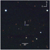 |
Fig. 1. A griz-color composite image of SN 2020bqj and its environment, as observed with LT/IO:O on 2020 March 6, +32 days after estimated explosion epoch. The SN outshines its faint host. |
Milky Way (MW) extinction towards the SN is estimated to be E(B − V) = 0.0194 mag (Schlafly & Finkbeiner 2011). All photometry are corrected for MW extinction adopting the Cardelli extinction law (Cardelli et al. 1989) with RV = 3.1. We assume host galaxy extinction towards the SN is negligible as the spectra do not show evidence of Na I D absorption lines.
2.2. Photometry
2.2.1. Optical
Photometry was obtained with the ZTF camera mounted on the P48 telescope from nominal ZTF survey observations: the public Northern Sky Survey with a 3 day cadence in g- and r-band (Bellm et al. 2019b) and the ZTF Uniform Depth Survey (ZUDS, Goldstein et al., in prep.) at a nightly cadence in g-, r- and i-band from MJD 58954 onwards. Additional photometry was obtained from Palomar with the Spectral Energy Distribution Machine (SEDM; Blagorodnova et al. 2018) mounted on the Palomar 60 inch telescope (P60; Cenko et al. 2006). The P48 data were reduced using the ZTF pipeline (Masci et al. 2019) and image subtraction based on the Zackay et al. (2016) algorithm, which produces template subtracted PSF photometry in the Sloan Digitial Sky Survey (SDSS) photometric system calibrated against field stars selected from the Pan-STARRS1 survey (Chambers et al. 2016). The P60 photometry was produced using the pipeline described in Fremling et al. (2016). Additional optical photometry in ugriz was obtained with the Infrared-Optical imager (IO:O) on the LT. The observed optical photometry is listed in Table A.1 and the lightcurve, corrected for MW extinction, is shown in Fig. 2. The phase presented in the lightcurve figure and this work, unless otherwise stated, is rest-frame days since the estimated explosion epoch, which we adopt to be halfway between the last non-detection and the discovery epoch, i.e. at MJD = 58880.0 ± 1.5.
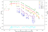 |
Fig. 2. Lightcurves of SN 2020bqj, corrected for MW extinction. Non-detections with 5σ upper limits are indicated by triangles. Apparent magnitudes on the left hand axis and absolute magnitudes to the right. The photometry on the decline has been binned in three-night bins. Phase is rest-frame days since the estimated explosion epoch, which was assumed to fall halfway between latest non-detection and discovery epoch. SwiftB- and V-band data are not shown due to their large photometric uncertainties. Bottom panel: g − r color evolution, which stays roughly constant throughout the evolution of SN 2020bqj except for possibly the first ∼5 days. |
2.2.2. UV
Follow-up in the ultraviolet (UV), starting at +41 days, was obtained with the UltraViolet and Optical Telescope (UVOT) aboard the Neil Gehrels Swift Observatory in the UVW2, UVM2 and UVW1 filters. Simultaneously, optical follow-up was obtained in the u, B and V-filters. The UVOT data were retrieved from the UK Swift Data Archive1 and reduced using standard software distributed with HEAsoft2. Photometry was measured using the FTOOLS tasks uvotimsum and uvotsource with a 5″ radius circular aperture. The host contribution has not been accounted for, but the contribution by the faint (r ∼ 23.5 mag) host is expected to be small, see Sect. 5.
The UV/optical photometry in AB magnitudes are listed in Table A.1 and the lightcurve is shown in Fig. 2.
2.3. Optical spectroscopy
An initial optical spectrum was obtained 4 days after discovery, using the SEDM on the P60 telescope. Additional optical follow-up spectroscopy was obtained using SEDM, the Dual Imaging Spectrograph (DIS3) mounted on the 3.5 m telescope at the Apache Point Observatory, the Alhambra Faint Object Spectrograph and Camera (ALFOSC) on the Nordic Optical Telescope (NOT; Djupvik & Andersen 2010), SPRAT on the LT, and the Low Resolution Imaging Spectrograph (LRIS; Oke et al. 1994) on the Keck I telescope. The spectroscopic coverage of SN 2020bqj presented in this paper consists of 16 spectra and extends from 4 days until 117 days after discovery in the observer frame.
The spectra were reduced in a standard manner using pipelines and procedures specific for each instrument, such as PYSEDM (Rigault et al. 2019) for the SEDM spectra, the PYDIS package (Davenport et al. 2018) for APO/DIS, and LPIPE (Perley 2019) for Keck/LRIS. Data reduction involved bias and flat-field corrections, wavelength calibration from an arc spectrum, and flux calibration using spectrophotometric standard stars. Furthermore, all spectra were absolute flux calibrated by matching their synthetic photometry with our observed r-band photometry. The spectra were then corrected for MW extinction using E(B − V) = 0.0194 mag and RV = 3.1. The spectral sequence is listed in Table A.2 and shown in Fig. 3. All spectra will be made available via WISeREP (Yaron & Gal-Yam 2012).
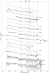 |
Fig. 3. Spectral sequence of SN 2020bqj, see Table A.2. Phases are relative to the estimated explosion epoch, halfway between the last non-detection and the discovery epoch. Some spectra have been smoothed with a median filter for clarity. A selection of prominent emission lines are indicated. |
2.4. X-ray and radio
The SN was observed with the X-ray telescope (XRT; Burrows et al. 2005) on-board Swift between 2020 March 9 (+35 days) and 2020 May 31 (+113 days). We analyzed all data with the online-tools of the UK Swift team4 that use the methods described in Evans et al. (2007, 2009) and the software package HEAsoft. The SN evaded detection in all Swift pointings. The nominal 3σ count-rate limit varies between 0.004 and 0.03 ct s−1 (0.3 and 10 keV; not corrected for absorption). Using the dynamic rebinning option, the 3σ between 2020 March 9 and 2020 May 31 is 5 × 10⁻⁴ ct s−1 (0.3−10 keV; not corrected for absorption). If we assume a power-law shaped spectrum with a photon index of 2 and a Galactic absorption of 1.67 × 1020 cm−2 (HI4PI Collaboration 2016), this corresponds to an absorption-corrected flux of 1.4 × 10⁻¹⁴ erg cm−2 s−1 between 0.3 and 10 keV. At the luminosity distance of SN2020bqj, this flux limits translates to a luminosity of < 2 × 1041 erg s−1.
We obtained one epoch at radio wavelengths on 2020 March 9 (+35 days) with the Arcminute Microkelvin Imager Large Array (AMI-LA; Zwart et al. 2008; Hickish et al. 2018). AMI-LA is a radio interferometer comprised of eight, 12.8 m diameter, antennas producing 28 baselines which extend from 18 up to 110 m in length and operates with a 5 GHz bandwidth around a central frequency of 15.5 GHz. Initial data reduction, flagging and calibration of the phase and flux, were carried out using reduce_dc, a customized AMI-LA data reduction software package (e.g., Perrott et al. 2013). Phase calibration was conducted using short interleaved observations of J1527+3115, while 3C286 were used for absolute flux calibration. Images of the field of SN 2020bqj were produced using CASA task CLEAN in an interactive mode, while the image rms was calculated using CASA task IMSTAT. No source was detected with a 3σ limit of 81 μJy. This corresponds to an upper limit of νLν ≤ 1.3 × 1038 erg s−1, given the luminosity distance of SN 2020bqj.
3. Photometric analysis
3.1. Early phase lightcurve
SN 2020bqj reached its plateau magnitude in r-band at the second epoch (+4.2 days), with Mr = −19.23 ± 0.07, whereas in g-band the plateau had already been reached at the discovery epoch (+1.4 days), with Mg = −19.43 ± 0.07, see Fig. 4. Based on the last pre-discovery limits the risetime to the peak plateau in r-band is constrained to < 5.7 days in rest-frame. Such a photometric evolution is typical for a rapidly-evolving SN Ibn, as depicted by the g- and r-band lightcurves of SN 2018bcc, a SN Ibn with a particularly well-sampled rise to peak (Karamehmetoglu et al. 2021). Also shown in Fig. 4 is the Type Ibn R/r-band template lightcurve constructed by Hosseinzadeh et al. (2017), based on a sample of 18 Type Ibn SNe from the intermediate Palomar Transient Factory (iPTF; Kulkarni 2013) and the literature. The absolute r-band magnitude of SN 2020bqj of the peak plateau is consistent with the peak of the SN Ibn template. The rise to the peak plateau of SN 2020bqj is fast compared to the template, but as noted in Hosseinzadeh et al. (2017) the early phases of the SN Ibn template are biased due to the limited number of SNe Ibn in the literature with pre-peak coverage and not taking into account upper limits. As such, a better comparison is with the lightcurve of SN 2018bcc. The first r-band data point of SN 2018bcc shown in Fig. 4 was not included in the initial study by Karamehmetoglu et al. (2021), but recovered after re-analysis of the data.
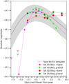 |
Fig. 4. g- and r-band lightcurves of SN 2020bqj (in green and red) and Type Ibn SN 2018bcc (in lime and magenta) from Karamehmetoglu et al. (2021) and Type Ibn R/r-band template lightcurve from Hosseinzadeh et al. (2017) at early phase. The lightcurve of SN 2020bqj in g- and r-band in its first fifteen days is consistent with those of Type Ibn SNe, albeit relatively fast in its rise. SN 2020bqj reached a r-band magnitude of the plateau consistent with the peak magnitude of the Ibn template, with a risetime constrained to < 5.7 days in rest-frame by pre-discovery upper limits. While this is fast compared to the template, it matches well with the risetime of SN 2018bcc. |
3.2. Plateau phase and decline
After the initial rise, the lightcurve of SN 2020bqj enters a plateau phase in g-, r- and i-band that lasts for 40 days at an r-band absolute magnitude ranging between −19.1 and −19.3. The plateau phase is followed by a linear decline lasting > 90 days with a rate of ∼0.04 mag day−1. Such a post-peak evolution is in contrast with what is commonly observed in SNe Ibn, where a quick rise to peak is followed by a fast decline at a rate of ∼0.1 mag day−1 (Hosseinzadeh et al. 2017).
The full r-band lightcurve of SN 2020bqj and the R/r-band SN Ibn template are shown in Fig. 5. Where most SNe Ibn have declined ∼4 mag at 40 days after peak, SN 2020bqj stayed at a similar magnitude throughout. Also plotted are the lightcurves of four other photometric outliers in the SN Ibn subclass. These SNe have irregular photometric evolution reminiscent of SN 2020bqj, showing either a double peak or a plateau phase, and were not included in the construction of the R/r-band SN Ibn template. The sub-luminous OGLE-2014-SN-131 displayed a slow evolution both in the rise and the decline, peaking at an r-band magnitude of Mr ≈ −18 (Karamehmetoglu et al. 2017). SN 2011hw was first detected at a magnitude of Mr ≈ −18.5, at which the SN stayed for ∼30 days, after which a linear decline set in with a rate of 0.055 mag day−1 (Smith et al. 2012; Pastorello et al. 2015b). No pre-discovery limits were available for SN 2011hw, so the risetime and phase is unknown, but based on its spectral evolution Pastorello et al. (2015b) estimated the explosion epoch to have occurred 14 ± 10 days before discovery, which we adopt in the figure. iPTF13beo reached peak magnitude 4 days after the last pre-explosion non-detection, and a second peak was observed ∼9 days after the first (Gorbikov et al. 2014). SN 2005la was discovered after peak, and its lightcurve showed re-brightening twice during the subsequent decline (Pastorello et al. 2008b). No stringent upper limits before the discovery of SN 2005la were available, preventing a well constrained estimate of the explosion epoch. The final remaining photometric outlier in the SN Ibn subclass is not shown here, since OGLE-2012-SN-006 showed a monotonic evolution similar to that of a regular SN Ibn, but at a considerable slower pace (Pastorello et al. 2015c). Finally, we also show PTF11rfr, a SN IIn which rose to peak rapidly for its subclass, followed by a peak plateau and a slow decline at ∼0.01 mag day−1 (Nyholm et al. 2020).
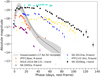 |
Fig. 5. Type Ibn R/r-band template lightcurve from Hosseinzadeh et al. (2017), with overplotted the r-band lightcurve of SN 2020bqj (in black) and the R/r/I-band lightcurves of the slow evolving and/or double-peaked SNe Ibn OGLE-2014-SN-131 (yellow), SN 2011hw (blue), iPTF13beo (orange) and SN 2005la (purple). Also shown is PTF11rfr (turquoise), a rapidly rising SN IIn with a peak plateau, but a slow decline (see Nyholm et al. 2020). The latest pre-discovery upper limits, where available, are indicated by triangles. While normal Type Ibn SNe have declined ∼4 mag 35−40 days after peak, SN 2020bqj stayed constant in brightness during the same period. SN 2011hw shows a similar lightcurve evolution, albeit one magnitude fainter. Phase is days in rest-frame since estimated explosion epoch for SN 2020bqj, SN 2011hw, iPTF13beo. The phases of SN 2005la, OGLE-2014-SN-131 and PTF11rfr are relative to their last non-detections, although for the two SNe Ibn these observations were rather shallow. The phase of the Type Ibn template is relative to the start of the template at 8 days before peak. |
3.3. Pseudo-bolometric lightcurve
A large fraction of the photometric coverage of SN 2020bqj, from +35 days to +114 days, extends from the UV to z band, covering the spectral range from ∼1600 to ∼11 000 Å. This allows us to simply integrate the spectral energy distribution (SED) using trapezoidal integration to obtain a pseudo-bolometric lightcurve that covers most of the SN flux. We interpolate the gaps in the photometric coverage in the different filters in this period using Gaussian Processes (GP) interpolation with GPy5. We used multi-task GP with a radial basis function kernel to capture the smooth evolution characterized by a typical length scale, and a linear and bias kernel to capture the decline. The fits were performed in flux space with an additional white noise kernel to model the intrinsic scatter. This method will be explained in detail in Karamehmetoglu et al. (in prep.). In this way we obtain lightcurves at a nightly cadence in all filters, the integrated flux of which is used to construct the pseudo-bolometric lightcurve.
Then, we extrapolate the pseudo-bolometric lightcurve to < +35 days by applying a bolometric correction to the (interpolated) flux captured in g band, where we assume that the shape of the SED of the SN does not change significantly over time. This assumption is supported by the lack of color evolution in the lightcurve (see Fig. 2), and the weak spectral evolution (see Fig. 3 for the spectral sequence). We note that at very early times this assumption may not be correct as the SN appears bluer in the first epoch (Fig. 2).
The resulting pseudo-bolometric lightcurve is shown in Fig. 6. It is not a full bolometric lightcurve as we do not account for the SN flux in the far-UV and near-IR not covered by our photometry, but based on blackbody fits to the broadband photometry we estimate this to be < 10% of the SN bolometric flux. Additionally, the pseudo-bolometric lightcurve does not extend to the faint end of the lightcurve past +114 days, since due to the larger uncertainties in the photometry and a lack of UV data, the faint linear tail does not meaningfully constrain the model fits discussed in Sect. 6. The total observed radiated energy from discovery to +114 days is 1.1 ± 0.1 × 1050 erg. This can be considered a conservative lower limit to the total energy radiated by the SN in this period, since it does not include flux in the far-UV and IR, and the blue colors at early phases suggest a higher photospheric temperature and thus higher luminosity than was extrapolated.
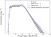 |
Fig. 6. Pseudo-bolometric lightcurve of SN 2020bqj based on trapezoidal integration of the broadband fluxes. Overplotted are TIGERFIT model fits (see Sect. 6). The radioactive 56Ni decay model fit has t0 set to −2 days before our adopted estimated explosion epoch. The hybrid CSM+Ni model fits shown assume a CSM shell (s = 0) or a wind profile (s = 2), with t0 set to −4 and −3 days, respectively. The radioactive decay model does not reproduce the transitions between the rapid rise, plateau and decline phases. The hybrid models recover the shape of the lightcurve much better, in particular the Ni+CSM shell (s = 0) model shows similar sharp transitions as the data. None of the models recover the rapid rise from the latest non-detection to discovery 2.8 rest-frame days later. Phase is relative to estimated explosion epoch. |
4. Spectral analysis
4.1. Line identification
Throughout the evolution of SN 2020bqj the spectra of the SN are dominated by intermediate-width emission lines (∼2000 km s−1, further discussed in Sect. 4.2). The initial low resolution SEDM spectrum obtained at +5 days (as with the lightcurve, phase is rest-frame days since estimated explosion epoch) did not allow for a secure classification of the object, but based on subsequent spectra the prominent emission lines in the earliest spectrum can be identified as He Iλλ5876, 7065, and C IIλ7231−7236, see Fig. 3. In the noisier blue end of the spectrum also C IIλλ3920,4267 can be identified, where the bluest line is likely merged with He Iλ3888. Subsequent spectra continue to show the same strong He I emission lines, as well as C II, most prominently at 7231−7236 Å.
The high signal-to-noise (SNR) spectrum obtained at +47 days with Keck allows for secure line identifications and line velocity measurements, see Fig. 7. FWHM line velocities were measured by fitting a Gaussian line profile, with errors dominated by the resolution of our low-resolution spectrographs. In addition to He Iλλ5876, 7065, the Keck spectrum shows clear He I in emission at λλ3888, 5016, 6678 and 7281, with line velocities ranging from vFWHM = 1500 ± 130 km s−1 for He Iλ7281 to vFWHM = 2680 ± 130 km s−1 for He Iλ5876. Hα and Hβ are visible, with Hα possibly merged with faint C IIλ6580 (see Sect. 4.2). Assuming Hα dominates this emission feature, the mean Balmer velocity is vFWHM = 2370 ± 140 km s−1, consistent with He Iλ5876. Although weak at this epoch, C IIλ4267 and C IIλ7231−7236 are still discernible, where the latter line is blended with He Iλ7281. By fitting two Gaussians simultaneously, we measure a velocity of vFWHM = 1870 ± 140 km s−1 for C IIλ7231−7236. C I is detected at λλ8335, 9094−9111 and 9405, with a velocity of vFWHM = 1380 ± 160 km s−1. O I at 7772−7775 Å and 8446 Å are present, the latter of which has a velocity of vFWHM = 2030 ± 160 km s−1. Mg II at λλ7877−7896 and λλ8213−8234 are visible, as well as at λλ9218−9244 potentially merged with O Iλ9266. The steep pseudo-continuum bluewards of ∼5700 Å is typical for SNe Ibn post-peak, and is attributed to the blending of a forest of Fe lines (Smith et al. 2012; Stritzinger et al. 2012; Pastorello et al. 2015b). Finally, the position of the Ca II triplet is indicated, which is not observed yet at this epoch, but does become prominent at later times, see Fig. 3.
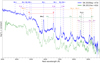 |
Fig. 7. High signal-to-noise spectrum of SN 2020bqj obtained with Keck at +47 days after estimated explosion epoch, with all emission lines discussed in the text identified. Also shown is a TNG/DOLORES spectrum of the peculiar SN 2011hw obtained +42 days after estimated explosion epoch (Pastorello et al. 2015b). SN 2011hw is a SN Ibn with a photometric and spectroscopic evolution that is very similar to SN 2020bqj, albeit somewhat faster. For example, the Ca II triplet is already visible in SN 2011hw, while in SN 2020bqj this feature only shows up from +71 days onwards (Fig. 3). |
Also shown in Fig. 7 is a TNG/DOLORES spectrum of SN 2011hw (Pastorello et al. 2015b), a peculiar SN Ibn with a photometric evolution similar to that of SN 2020bqj, see Sect. 3.2. This spectrum was obtained at a similar epoch as the Keck spectrum of SN 2020bqj, just after the decline has set in, and is remarkably similar. All aforementioned lines were also observed in SN 2011hw, although O I is weaker, Mg II more prominent, and Ca II is already visible (in SN 2020bqj Ca II is not observed until at +71 days, see Fig. 3). The intermediate-width He I lines in SN 2011hw have a similar velocity (∼1900 km s−1, Smith et al. 2012) as SN 2020bqj. The spectra comparison also allows us to identify the weak narrow (unresolved, ≲300 km s−1) feature blue-wards of He Iλ5876 as [N II] λ5754, which was also detected in SN 2011hw (Pastorello et al. 2015b). It is worth noting that C I and C II are also visible in the SN 2011hw spectrum, although this was not reported in the original studies (Smith et al. 2012; Pastorello et al. 2015b). In particular at early epochs the spectra of SN 2011h show prominent C II, which is further discussed below.
4.2. Spectral line evolution
Figure 8 shows the evolution of some of the most prominent emission lines in the spectra of SN 2020bqj. In summary, throughout the spectral sequence He Iλ5876 and He Iλ7065 remain prominent, whereas the C IIλ7231−7236 emission line decreases in strength over time and appears to have completely disappeared at +71 days. The line feature at 6580 Å at early epochs likely consists of Hα and C IIλλ6578−6582, but by +47 days in the high SNR Keck spectrum the emission feature is well described by a single Gaussian centered on Hα, implying C IIλλ6578−6582 has faded away.
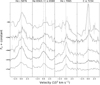 |
Fig. 8. Line evolution of prominent emission lines in the spectra of SN 2020bqj. From left to right: He Iλ5876, Hα merged with C IIλ6580, He Iλ7065 and C IIλ7231−7236. |
We quantified the evolution in line strength and velocity of the He Iλλ5876, 7065 and C IIλ7231−7236 lines by fitting a Gaussian line profile. A flat continuum around the line was assumed and derived by fitting the region surrounding the emission line, while excluding the emission line itself. We then fit a Gaussian to the line after subtracting the straight-line continuum. We obtained FWHM velocities and pseudo-Equivalent Widths (pEWs) from our Gaussian fits using standard formulae. We corrected the Gaussian σ for instrumental resolution of each spectrum at the position of the line. All fits were visually inspected and any poor fits were removed. This was usually due to poor SNR at the line position from a noisy spectrum. In addition, the fits to the P60 spectra, which have very low instrumental resolution, are not included in our analysis. The statistical uncertainties of the fits were derived from the fitting errors. However, these are only a minor source of uncertainty in fitting emission lines. The dominant source of uncertainty arises from the inability to distinguish the continuum from the line. As an estimate for this source of uncertainty, we used the FWHM of the instrumental resolution at the position of the respective line, added in quad with the fitting errors. The reason we used the instrumental resolution as a proxy for this uncertainty is because the resolution acts as a natural measure of line blending, which is one of the main reasons why separating the continuum from the line is so difficult.
The resulting pEW evolution is shown in Fig. 9. Table 1 lists the pEW and vFWHM, with the low resolution SEDM spectra and poor line fits omitted.
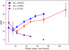 |
Fig. 9. Evolution of the pEW for the He Iλλ5876, 7065 and C IIλ7231−7236 emission lines. P60 spectra have not been analyzed due to their lower resolution. Fits to low SNR lines are excluded, especially for the latter spectra. |
Line velocities and pseudo equivalent width of the He Iλλ5876, 7065 and C IIλ7231−7236 emission lines.
The first trend in the He I lines that is worth noting is the evolution of the relative pEW of He Iλ5876 and He Iλ7065. While He Iλ5876 initially has twice the pEW of He Iλ7065, both become stronger with time and this difference seems to lessen. In addition, He Iλ7065 is weak or possibly absent in our first spectrum at +8 days, while He Iλ5876 is clearly present. An evolution of He Iλ7065 becoming relatively stronger with time and growing to match He Iλ5876 is also observed in other SNe Ibn (e.g. Karamehmetoglu et al. 2021) and is an indication of very high electron densities in the post-shock shell (Almog & Netzer 1989; Smith et al. 2012). Secondly, the FWHM velocities of He Iλ7065 are significantly slower than those of He Iλ5876.
The pEW and velocity evolution of the C IIλ7231−7236 line doublet is markedly different. Initially the line is possibly even stronger than He Iλ5876, which despite the large uncertainty of the pEW measurement (the line is barely resolved in the LT/SPRAT spectrum) is also apparent in the spectral sequence shown in Fig. 8. Subsequently, the line strength of C II decreases and by the time of the NOT spectrum at +71 days, it is impossible to say whether the C IIλ7231−7236 line is still present or not with a pEW and line velocity consistent with zero. As discussed previously, a similar behavior is observed in all C lines we observe. Additionally, the line velocity of C IIλ7231−7236 is consistently lower than that of He Iλ5876 by ∼1700 km s−1, which is especially noticeable in the early spectra.
C II emission lines are not commonly observed in SNe Ibn, but as discussed earlier they featured in early spectra of SN 2011hw. Additionally, an early spectrum of PS1-12sk (Sanders et al. 2013) showed intermediate-width (∼2000 km s−1) C II, and broad C II (possibly merged with He Iλ7281) was observed in LSQ13ccw (Pastorello et al. 2015a). Interestingly, both SN 2011hw and PS1-12sk are considered outliers in the SN Ibn subclass based on photometric evolution and host galaxy properties, respectively, and both showed Hα as well. In Fig. 10 we show early spectra of SN 2011hw and PS1-12sk compared to spectra of SN 2020bqj at similar epochs, as well as the prototypical Type Ibn SN 2006jc (Foley et al. 2007). Phases are relative to estimated explosion epochs. As with SN 2011hw (Sect. 3.2), the explosion epochs of SN 2006jc and PS1-12sk are poorly constrained. For PS1-12sk we adopt the estimated explosion epoch of MJD = 55992 ± 5 from Hosseinzadeh et al. (2017), and for SN 2006jc we adopt as explosion epoch MJD = 54004, halfway between last non-detection and the estimated peak epoch of MJD = 54008 from Hosseinzadeh et al. (2017).
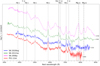 |
Fig. 10. Spectrum of SN 2020bqj at +23 days, together with spectra of the prototypical SN Ibn 2006jc and the peculiar SNe Ibn SN 2011hw and PS1-12sk, at similar epochs since estimated explosion. SN 2020bqj, SN 2011hw and PS1-12sk show similar features across the spectrum, including prominent C II lines, which are not observed in SN 2006jc. The C II features in the spectrum of PS1-12sk have disappeared at +26 days (see Sanders et al. 2013), whereas for SN 2020bqj and SN 2011hw they remained visible for ∼50 days. |
At ∼22 days past explosion, SN 2020bqj, SN 2011hw and PS1-12sk all show very similar features across the spectrum, featuring prominent intermediate-width C II and Hα in addition to the canonical He lines. As with SN 2020bqj, the C II emission lines fade away with time, although at different rates. A spectrum obtained of PS1-12sk at +26 days showed C IIλ7231−7236 as an absorption feature instead (Sanders et al. 2013), while the same feature was weak but still observed at ∼+45 days in both SN 2020bqj and SN 2011hw, see Fig. 7. No carbon lines were ever reported for SN 2006jc. Sanders et al. (2013) attributed the initial presence and fast decline of C II to an effective temperature dependence, as is observed in Type Ia SNe (Parrent et al. 2011). Such a temperature decrease is seemingly in conflict with the lack of color evolution of SN 2020bqj (Fig. 2). This may suggest that the lack of color evolution is a result of (ongoing) CSM interaction features dominating the SN spectrum, such as the pseudo-continuum due to Fe lines in g-band. The only Balmer line detected in SN 2006jc was a weak Hα emission line that increased slightly in line strength throughout its evolution (Foley et al. 2007). SN 2020bqj, SN 2011hw and PS1-12sk also all show Hα increasing with time (Smith et al. 2012; Sanders et al. 2013), but the line is much more prominent in SN 2020bqj and SN 2011hw, particular at late epochs, see Fig. 7.
Finally, studying the evolution of the different velocity components in the emission lines of interacting SNe provides a method to constrain the properties of the CSM and origin of the line-emitting regions. Intermediate-width (∼few × 103 km s−1) and broad (up to ∼104 km s−1) emission lines in SNe Ibn are thought to originate from either the shock front between SN ejecta and CSM, or from the freely expanding SN ejecta, respectively (Pastorello et al. 2016).
The velocities of the intermediate-width He emission lines of SN 2020bqj evolve only slowly over time (Table 1), and show no evidence of a broad P-Cygni profile. Based on this, we interpret the intermediate-width emission lines of ∼2500 km s−1 to be that of the shocked gas, rather than the SN ejecta. Narrow (102 − 103 km s−1) velocity components superimposed on the strong He lines, such as observed in SN 2011hw (Smith et al. 2012), likely trace unshocked slow-moving CSM. The velocity of the unperturbed CSM can be determined from the narrow emission line widths, or inferred from the blueshifted absorption minimum of a narrow P-Cygni profile, if present (Pastorello et al. 2016). SN 2020bqj shows some evidence of narrow emission features superimposed on broad He lines, but they are weak and unresolved. However, weak blue-shifted absorption superimposed on the strong emission lines is observed in for example He Iλ5876 (Fig. 8). We measure from a selection of He lines in the +47 days Keck spectrum an absorption velocity of 230 ± 130 km s−1, relative to the intermediate-width emission line centers. Based on the analysis of similar features in SN Ibn LSQ13ddu (Clark et al. 2020) in low and high resolution spectra, this velocity can be considered an upper limit to the velocity of the unperturbed CSM around SN 2020bqj due to our lack of spectra with high spectral resolution.
5. Host galaxy
To investigate the properties of the host galaxy of SN 2020bqj we modeled its SED based on archival data retrieved from the Legacy Surveys (Dey et al. 2019). We measured the brightness of the host using the aperture photometry tool presented in Schulze et al. (2018) that is based on Source Extractor version 2.19.5 (Bertin & Arnouts 1996). To calibrate the instrumental magnitudes, we measured the brightness of stars from SDSS in the same way. The observed AB magnitudes (not corrected for extinction) of the host obtained this way are g = 23.38 ± 0.18, r = 23.46 ± 0.40 and z > 22.2. We modeled the SED with the software package prospector version 0.3 (Leja et al. 2017). Prospector uses the Flexible Stellar Population Synthesis (FSPS) code (Conroy et al. 2009) to generate the underlying physical model and python-fsps (Foreman-Mackey et al. 2014) to interface with FSPS in python. The FSPS code also accounts for the contribution from the diffuse gas (e.g., H II regions) based on the Cloudy models from Byler et al. (2017). Furthermore, we assumed a Chabrier initial mass function (Chabrier 2003) and approximated the star formation history (SFH) by a linearly increasing SFH at early times followed by an exponential decline at late times (functional form t × exp(−t/τ)). The model was attenuated with the Calzetti et al. (2000) model. Finally, we use the dynamic nested sampling package dynesty (Speagle 2020) to sample the posterior probability function.
The derived mass and star-formation rate of the galaxy are  and SFR =
  yr−1, respectively. The values represent the median of the posterior probability function and 1σ errors. The best-fit SED has a reduced χ2 of 3.5 for three filters. Based on the derived parameters, the host of SN 2020bqj is an outlier in the SN Ibn subclass, with in particular a low galaxy mass. This is demonstrated in Fig. 11, where the derived properties of the host of SN 2020bqj are shown together with those of a sample of SN Ibn hosts from iPTF, where mass and SFR was derived in a consistent way (Schulze et al. 2021). The host galaxy masses of the nine SNe Ibn observed in iPTF ranged between 108 to 1010 M⊙, which puts the mass of the host of SN 2020bqj two orders of magnitude lower than the least massive SN Ibn host in iPTF. In terms of total SFR, the host of SN 2020bqj is low but within uncertainties consistent with the lower end of the SFR distribution of the iPTF sample. As a consequence of its very low mass, the host of SN 2020bqj falls above the galaxy main sequence, a fundamental correlation between SFR and mass of star-forming galaxy (Lee et al. 2015). The specific SFR of the host, SFR normalized by stellar mass, is high in comparison with the iPTF host sample, and in the range of starburst galaxies. Finally, at a distance of 297 Mpc, the host has an absolute magnitude of Mr = −14.35, which is considerably fainter than the sample discussed in Pastorello et al. (2015c) of actively starforming spirals that typically host SNe Ibn.
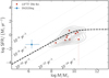 |
Fig. 11. The host galaxy of SN 2020bqj in the mass–SFR plane. The hosts of SNE Ibn from the iPTF survey (Schulze et al. 2021) have masses between 108 and 1010 M⊙ and lie in the region of the galaxy main sequence, a fundamental correlation between SFR and mass of star-forming galaxies (thick dashed line; Lee et al. 2015). To guide the eye, contours from 10% to 90% based on the iPTF sample are overlaid. The mass of SN 2020bqj’s host stands out from this comparison sample. Its mass is more than 2 dex lower than the least massive host of that sample, albeit the errors are large. The grey-dashed lines display lines of constant specific star-formation rate (SFR normalized by stellar mass). |
In conclusion, SN 2020bqj was hosted by an unusually faint and small galaxy for a SN Ibn host. Here it must be noted that the SED model of the host is based on sparse archival SN-free imaging. In order to further constrain the hosts properties, deep imaging and spectroscopy are required, to be obtained after the SN has faded. Such follow-up would also allow for the determination of the physical size of the host, and then a direct comparison of its SFR density with those of the sample of SN Ibn hosts presented by Hosseinzadeh et al. (2019). Constraints on the host galaxy metallicity would also be useful, as a low metallicity environment has implications on the progenitor, and its mass-loss rate, of SN 2020bqj. Interestingly, the prominent outlier in the study by Hosseinzadeh et al. (2019) in terms of host galaxy properties, PS1-12sk, was a SN Ibn discovered in an elliptical cluster galaxy at a site of extremely low local SFR density. As discussed in Sect. 4 and shown in Fig. 10, PS1-12sk is spectroscopically very similar to SN 2020bqj.
6. Powering mechanism
Normal Type Ib/c SE SNe have lightcurves that are well fitted by 56Ni decay powered models (e.g., Prentice et al. 2016). The lightcurves of SNe Ibn usually call for a different and/or additional power source, because the amount of 56Ni required to explain their peak luminosity can not be reconciled with the steep decline rate of SNe Ibn. Although the decline rate of SN 2020bqj is much slower, the sharp transitions between rise, plateau and decline in the lightcurve of SN 2020bqj do not match with the monotonic evolution of a radioactive decay dominated lightcurve. In the spectra of SN 2020bqj intermediate-width emission lines are visible throughout the full lightcurve evolution (Fig. 3), so it is only natural to assume CSM interaction plays an important role in the powering of the peculiar lightcurve of SN 2020bqj.
We investigate the powering mechanism of SN 2020bqj by fitting the lightcurve with (a combination of) semi-analytical lightcurve models. We employ photometric modeling codes that have these models incorporated to provide fits to the SN lightcurve. First, we explore different models with TIGERFIT (Chatzopoulos 2018), where the best-fit model to a bolometric lightcurve of a transient is determined via χ2 minimization. Then, we use the Monte-Carlo code MOSF IT (Guillochon et al. 2018) to fit the full lightcurve across all filters with the model(s) that recovered the bolometric lightcurve best in the fits with TIGERFIT. As a Monte Carlo code, MOSF IT has the advantage of providing more robust statistical uncertainties, and also explicitly treats and fits for all variables (including, e.g., explosion epoch). Unlike TIGERFIT it also takes into account color information by fitting each band individually. However, it is significantly more computationally expensive, particularly for a data set the size of SN 2020bqj.
6.1. TigerFit
TIGERFIT requires as input the phase in rest-frame since the explosion epoch, the bolometric luminosity (which we sample here at a daily cadence) and the associated uncertainty. For each model we fit for phases with discrete offsets t0 from our adopted explosion epoch (MJD = 58880) of t0 = [0, −1, −2, −3, −4, −5] days, and consider here the models with the lowest χ2 that still adhere to the upper limit on the luminosity from the last non-detection. We consider a radioactive decay model assuming diffusion into homologously expanding SN ejecta based on Arnett (1980, 1982), and the CSM interaction model described in Chatzopoulos et al. (2012, 2013), which includes a large number of free parameters such as opacity κ (assumed constant), ejecta mass Mej, CSM mass MCSM and CSM density ρCSM. The ejecta density profile in the CSM model from Chatzopoulos et al. (2012) is described separately for the inner and outer ejecta, as ρej ∝ r−δ and ρej ∝ r−n, respectively. We adopt δ = 1 and n = 11, noting that the results are not very sensitive to these parameters. The density profile of the CSM is described as ρ ∝ r−s, where s = 0 corresponds to a CSM shell of constant density (the ‘shell’ model), and s = 2 corresponds to a profile that better describes a wind (the ‘wind’ model). We fit for both s = 0 and s = 2.
Figure 6 shows the resulting model fits to the data, including the radioactive decay model fit, and hybrid model fits of radioactive decay plus either the CSM shell or wind model. Fits using only the CSM interaction model are not shown here, since they did not represent the data well using reasonable parameters6. The radioactive decay model to the full bolometric lightcurve does not capture the different stages of the rise, plateau and decline of the lightcurve (reduced χ2/d.o.f. = 5.9, when t0 = −2), in particular not reproducing the sharp transitions between the three different stages. The Ni+CSM model fits recover the plateau much better, although depending on the CSM density profile the fits show different behaviors at early phases. Like the radioactive decay fits, the Ni+CSM fit with s = 2 rises monotonically, with the slope of the rise declining with time. The fit plotted in Fig. 6 assumes t0 = −3 days (reduced χ2/d.o.f. = 0.8). In contrast with the smooth evolution of the other models, the Ni+CSM shell model shows sharp transitions between the rise, a (concave) plateau feature, and the decline. The upper limit before discovery constrains t0 to −4 days, resulting in a reduced χ2/d.o.f. = 1.8 for the plotted fit. Both Ni+CSM model fits show a rise more rapid than the radioactive decay model, but neither are quite fast enough to fit the observed rise of SN 2020bqj.
While formally a slightly poorer fit, qualitatively the shell model with s = 0 recovers the shape of the bolometric lightcurve of SN 2020bqj remarkably well, with a fast rise, a plateau connecting two peaks, followed by a linear decline. The sharp transitions in the shell model originate from the behavior of the forward and reverse shock components that make up the Ni+CSM shell model. This is well demonstrated by Wheeler et al. (2017, their Fig. 1). The forward shock dictates the first half of the lightcurve, running through the CSM shell up until the transition between the rise and the (concave) plateau, when it reaches the outer edge of the CSM shell. The reverse shock dominates the later part of the lightcurve, with the transition between plateau and decline being the result of the shock reaching the interior of the ejecta. The following decline is a result of the diffusion from the shock-heated CSM matter. It is worth noting that the distinctive lightcurve features of SN 2020bqj that are so well recovered by this Ni+CSM shell model were also observed in SN 2011hw (Fig. 5), although its rise was not well constrained. The resulting parameters from fitting the bolometric lightcurve with the hybrid shell and wind CSM models in TIGERFIT are listed in Table B.1 for completeness, but should be considered secondary to the results obtained with MOSF IT in the following section.
From the TIGERFIT results we conclude the radioactive decay model does not reproduce the bolometric lightcurve well, and neither do models solely powered by CSM interaction. These models are thus rejected. Both hybrid Ni+CSM model fits (shell and wind) do recover the lightcurve well, although at early phases they show different behaviors. Next, we employ MOSF IT to fit the full multi-color lightcurve of SN 2020bqj, instead of the pseudo-bolometric lightcurve, with both Ni+CSM models. By fitting the individual bands directly with MOSF IT, we are less sensitive to the assumptions that went into constructing the pseudo-bolometric lightcurve, such as the lack of evolution of the SED of the SN during the first 35 days. Here it must be noted that MOSF IT assumes a blackbody SED, which may be reasonable for SN 2020bqj at early phases but less so after ∼15 days when the broader features, such as the typical SN Ibn pseudo-continuum, develop (Fig. 3).
6.2. MOSFiT
In the MOSF IT multi-band lightcurve fits of SN 2020bqj with the Ni+CSM models, the values for δ and n were adopted as above, and we allowed the progenitor radius and opacity to vary, resulting in a total of 12 free parameters in this model. We allowed all priors to vary over a wide range, regardless of the TIGERFIT results. As recommended for problems with a large number of free parameters, we use the dynamic nested sampler option in MOSF IT (implemented via the DYNESTY package; Speagle 2020). In either case, we initialize MOSF IT with 120 walkers, and allow it to run until it reaches the default stopping criterion in DYNESTY indicating that further sampling will no longer improve the evidence and posterior integrals (which took ∼28 000 iterations in the case of s = 0 and ∼31 000 iterations for s = 2).
The resulting lightcurve fits are shown in Fig. 12. The prior ranges and best estimates of the fitted parameter values relevant to our discussion are listed in Table 2. All listed parameters were well constrained by the data, with the uncertainties corresponding to the 68% confidence interval in the posterior distributions. The four unlisted parameters include a noise parameter σ, which for both models was well constrained and of similar value (σ ∼ 0.2), and two ‘nuisance’ parameters that are included to allow for a better determination of the more fundamental parameters such as ejecta mass and kinetic energy (Nicholl et al. 2017). These nuisance parameters, the gamma-ray opacity of the SN ejecta κγ and the H column density of the host nH, host are not well constrained by the data. The last unlisted parameter is the final plateau temperature Tf, to which the important physical parameters are not very sensitive (Nicholl et al. 2017). The corner plots associated with the two model fits are shown in Figs. C.1 and C.2.
 |
Fig. 12. Ni+CSM model lightcurves fitted to the photometry of SN 2020bqj using the Monte-Carlo code MOSF IT, with on the left the shell model (s = 0) and on the right the wind model (s = 2). A selection of lightcurves based on a random draw from the posteriors are plotted, to demonstrate the range of the model fit in each filter. The models are able to reproduce the flat plateau in the optical bands as well as the steady decline phase of the UV/optical. The rapid rise to the peak plateau of SN 2020bqj is less well reproduced, especially when taking into account the upper limits. |
Realized best estimates of eight free parameters used in fitting the hybrid Ni+CSM model to the multi-band lightcurve of SN 2020bqj with MOSF IT, and three derived parameters.
Both Ni+CSM models recover the plateau and decline phases of SN 2020bqj quite well. Neither of the model lightcurves recover the rapid rise of SN 2020bqj, in particular when accounting for the pre-discovery g- and r-band upper limits. Although upper limits are included in the fit, it is clear the optimal solution favors larger offsets of the free parameter t0 than with TIGERFIT, where t0 was fixed. We note that the upper limits reported here are global estimates of the full CCD (Masci et al. 2019), and may differ locally. As a very recent SN, it is not possible at this point to improve this estimate for the position of SN 2020bqj due to data access, but it is unlikely to change much given how faint the host of SN 2020bqj is. We used the dynesty sampler (Speagle 2020) in MOSF IT to sample the posterior probability function. The evaluation score, indicating how well a model fit the data, were similar for both models (103 and 107 for shell and wind model, respectively).
The first thing to note from the derived parameters in Table 2 is that the adopted density profile (wind or shell) of the CSM impacts some of the parameters significantly, while the produced lightcurves (Fig. 12) are not very different. This dependency on index s was already demonstrated by Chatzopoulos et al. (2013) and gives us the main caveat of the semi-analytical CSM model we use here: the actual CSM configuration around the SN is uncertain, so the results should not be taken literally but rather indicative, especially when showing large variations as a function of the adopted density profile.
The parameters that seem insensitive to the adopted density profile are mainly associated with the progenitor properties. Both model fits result in similar ejecta (15 M⊙ and 17 M⊙) and nickel masses (0.04 M⊙ and 0.03 M⊙). The ejecta velocity7 is larger in the wind model (8700 km s−1) as compared to the shell model (3300 km s−1), as a result of the larger kinetic energy of the SN in the wind model. The radius R0, which in this model corresponds to the inner radius of the CSM (Wheeler et al. 2017), and the upper limit of the radius of the progenitor, is poorly constrained in the shell model, ranging up to 3 AU, or ∼600 R⊙. Assuming a CSM velocity of ∼200 km s−1, this implies the shell was ejected very recently before explosion (< a month). Such an outburst has not been observed at the position of SN 2020bqj by ZTF, with coverage dating back two years (Strotjohann et al. 2021). However, at the distance of SN 2020bqj an outburst of similar brightness as that observed for the prototypical Type Ibn SN 2006jc (M = −14.0 mag, Nakano et al. 2006) would correspond to m = 23 mag, below the detection limit of nominal ZTF operations. The radius R0 in the wind model is better constrained, and of order ∼0.1 AU, or 22 R⊙.
The CSM masses show two orders of magnitude variation, and as such are much more uncertain. The large difference in CSM density ρCSM is expected, since it corresponds to the CSM density at the inner edge of the CSM at radius R0. In the shell model the density remains constant, while in the wind model it drops off as 1/r2. The derived CSM properties are a good demonstration of the uncertainty in the CSM configuration. A constant CSM density as in the shell model of 10−12 g cm−3 implies an electron density of ∼1010 cm−3, which is larger than observed in the line forming regions of Type IIn SNe (∼105 − 109 cm−3, e.g., Fransson et al. 2014). However, if the CSM originated from a wind, the mass-loss rate computed as  results in an extremely high mass-loss rate of Ṁ ∼ 1 M⊙ yr−1, where we assume vwind = 230 km s−1 inferred from the absorption velocity (Sect. 4). This mass-loss rate is much higher than typical mass-loss rates from steady-state winds of both LBV and WR stars (∼10−4 to ∼10−5, Smith 2017) and rather suggests more violent episodic mass-loss or outbursts. The actual configuration of the CSM is almost certainly more complicated than the two density profiles considered here.
Finally, we note that the MOSF IT and TIGERFIT results are not fully consistent, which is likely a result of systematic uncertainties resulting from fundamental assumptions in the two different methods, such as the extrapolation to early times in TIGERFIT and the shape of the SED in MOSF IT. However, in either case a large ejecta mass and a high opacity are required to recover the lightcurve of SN 2020bqj.
7. Discussion
SN 2020bqj is a clear outlier in the SN Ibn subclass, based on the combination of its unusual lightcurve, spectral features and host galaxy properties. Previous studies of ‘normal’ fast-evolving SNe Ibn have employed similar methods and models to model SN Ibn lightcurves as we have, which allows us to draw direct comparisons of our derived model parameters with their work. The ejecta mass of 15−17 M⊙ of SN 2020bqj inferred from the Ni+CSM models is similar to those derived for Type Ibn SN 2019uo (Gangopadhyay et al. 2020) and PS15dpn (Wang & Li 2020). The 56Ni mass of 0.03−0.04 M⊙ inferred from the modeling is comparable to the values for SN 2019uo and PS15dpn, as well as for the rapidly-evolving SE SN with narrow He features LSQ13ddu (Clark et al. 2020), and is consistent with the amount of 56Ni synthesized in the explosions of normal Type Ib/c SE SNe (e.g., Prentice et al. 2016). Since the ejecta and 56Ni masses are consistent with SNe Ibn with fast monotonically evolving lightcurves, it seems unlikely the explosion properties are the origin of the unusual lightcurve of SN 2020bqj.
Where the best fit model parameters of SN 2020bqj differ from those of the aforementioned SNe Ibn is in the properties of the CSM. The inner radius of the CSM, R0, of ∼0.1−0.3 AU (∼22 R⊙) is orders of magnitudes smaller than the radii derived for SN 2019uo, PS15dpn and LSQ13ddu. Also the inferred CSM optical opacity of κ ∼ 0.3 cm2 g−1 is higher for SN 2020bqj than in the model fits of these fast-evolving SNe Ibn (0.05−0.1 cm2 g−1). Interestingly, the lightcurve of the long-lived SN Ibn OGLE-2014-SN-131 (Fig. 5) was well represented by a CSM shell model with higher opacity of κ = 0.2 cm2 g−1 and a small radius of R = 1 R⊙ (Karamehmetoglu et al. 2017). Such an elevated opacity could be explained if the CSM not only contains He but also H (typical opacity κ ∼ 0.34 cm2 g−1). The presence of H in the CSM is supported by the (albeit faint) detection of Balmer lines in the spectra of OGLE-2014-SN-131, and they are also observed in SN 2020bqj (Fig. 8). In fact, an elevated H opacity was hypothesized by Smith et al. (2012) to explain the properties of the peculiar SN Ibn SN 2011hw, which seems to be an analog to SN 2020bqj both in terms of its lightcurve shape (Fig. 5) and the evolution of its spectra (Fig. 7). SN 2011hw was a well-studied event discussed by both Smith et al. (2012) and Pastorello et al. (2015b), and we consider here their interpretation of the properties of SN 2011hw in the context of SN 2020bqj.
Smith et al. (2012) compared the photometric and spectral properties of SN 2011hw to those of the prototypical Type Ibn SN 2006jc. The presence of more prominent Balmer lines and a 6000 K blackbody component (reminiscent of Type IIn SNe) in late time spectra of SN 2011hw, when compared to SN 2006jc, led Smith et al. (2012) to hypothesize that the main difference between SN 2011hw and SN 2006jc could be due to a slightly enhanced H-abundance in the CSM and the progenitor envelope of SN 2011hw. The stronger continuum H opacity would explain the higher luminosity and slower decline rate at late times of SN 2011hw as compared to SN 2006jc. The later appearance of Ca II (day 47 for SN 2011hw versus day 13 for SN 2006jc, Foley et al. 2007) would then be a result of the higher optical depths at large radii due to the elevated H abundance, hiding Ca II emission lines arising from the SN ejecta crossing the reverse shock. In comparison, the shape of the continuum and the Hα line strength of SN 2020bqj matches closely that for SN 2011hw (Fig. 7). The appearance of Ca II at +71 days is also delayed for SN 2020bqj (Fig. 3), even with respect to SN 2011hw. SN 2020bqj also shows the same distinctive lightcurve properties as SN 2011hw, and arguably more prominent. SN 2020bqj is brighter than SN 2011hw by ∼1 mag (Fig. 5), and its linear decline at 0.04 mag day−1 is slower than for SN 2011hw (0.055 mag day−1, Pastorello et al. 2015b).
The re-brightening of SN 2011hw at the end of the plateau was interpreted as additional luminosity input from the shock running into a denser portion of its CSM shell (Smith et al. 2012; Pastorello et al. 2015b). In the case of SN 2020bqj a similar secondary peak is well recovered by the Ni+CSM model (most prominently shown by the TIGERFIT shell model fit, Fig. 6) as the transition from the (concave) plateau phase to the decline phase due to the reverse shock reaching the interior of the ejecta, after which the lightcurve declines, dominated by the diffusion from the reverse shock heated matter (Wheeler et al. 2017). The lightcurve of SN 2011hw, where observed, is similar to that of SN 2020bqj in the plateau and decline phase. Therefore, we suggest that the light curve of SN 2011hw is dominated by shock heating in a scenario similar to that described for SN 2020bqj, rather than variations in the CSM density. Arguably this scenario could also be applied to the lightcurve of iPTF13beo, which showed a fast rise, double peak, and a subsequent decline (Fig. 5). The faster evolution of iPTF13beo compared to SN 2011hw and SN 2020bqj would then be a result of less H in the CSM, which is consistent with the lack of Balmer lines in the spectra of iPTF13beo (Gorbikov et al. 2014).
The elevated H abundance in the CSM of SN 2020bqj should reflect the composition of the envelope of the progenitor, since the CSM is assumed to have originated from the progenitor through mass-loss. The spectra of SN 2011hw showed narrow blue-shifted (by −80 to −250 km s−1) P-Cygni absorption features superimposed on strong emission lines. These absorption velocities correspond to the pre-shocked velocity of the CSM, and are unusually slow in SN 2011hw when compared to typical pre-shock CSM velocities of SNe Ibn (∼1000 km s−1, Pastorello et al. 2016). Smith et al. (2012) argued that the slower absorption velocities reflect a larger radius and thus lower escape velocity of its progenitor star than expected from classic, H-depleted WR stars (500−3200 km s−1, Crowther 2007), implying a progenitor with a higher H content such as an LBV (< 500 km s−1), which would be more consistent with a elevated H abundance in the CSM. Notably, Type Ibn SN 2005la (Pastorello et al. 2008b), which had a peculiar fluctuating lightcurve (Fig. 5), also showed slow unshocked CSM velocities (∼500 km s−1), as well as prominent Balmer lines. In SN 2020bqj we detected absorption features of ≲230 km s−1 in the high SNR spectrum obtained at +47 days (Sect. 4), which are consistent with mass-loss from an LBV star rather than a compact WR star. The inner radius of the CSM of SN 2020bqj inferred from the wind model (s = 2) of  can be considered an upper limit to the progenitor radius. Such a small radius would favor a more compact progenitor such as a WR star (Petrovic et al. 2006), but given the large uncertainties, it does not exclude an LBV star (e.g., Sholukhova et al. 2015).
Thus, the observed higher luminosity, slow wind speeds, slower decline rate, and delayed emergence of Ca II in SN 2020bqj would suggest a CSM with an elevated H-opacity compared to fast evolving SNe Ibn, similar to SN 2011hw, but potentially with an higher H-abundance. An elevated opacity is consistent with the model fits of the lightcurve of SN 2020bqj, where an opacity κCSM was derived of 0.25−0.31 g cm−3, depending on the model. Smith et al. (2012) and Pastorello et al. (2015b) suggested as progenitor options for SN 2011hw a massive star transitioning from the LBV to WR stage: either a early WN star with H or a member of the Ofpe/WN9 class of stars, which are very massive stars with ZAMS masses of 17−100 M⊙ (St-Louis et al. 1997). Such a massive progenitor, at a stage in its evolution between LBV and WR star where it has not yet lost most of its envelope through mass-loss, is consistent with the large ejecta mass of ∼15−17 M⊙ inferred for SN 2020bqj. In contrast, normal SNe Ib/c (the underlying SNe assumed for most SNe Ibn) are linked to evolved WR progenitors and have ejecta masses of order a few M⊙ (Drout et al. 2011; Lyman et al. 2016; Prentice et al. 2016; Barbarino et al. 2021). A scenario of a progenitor with LBV-like properties also suits the lightcurve and host galaxy of SN 2020bqj, since LBV stars have been linked to Type IIn SNe (e.g., Gal-Yam & Leonard 2009; Smith et al. 2010). Type IIn SNe display a variety of (long-lasting) lightcurves including SNe with plateaus similar to SN 2020bqj, such as PTF11rfr (Fig. 5; Nyholm et al. 2020). Additionally, the host galaxy of SN 2020bqj falls well within the distribution in host galaxy masses of Type IIn SNe (Schulze et al. 2021), whereas SN 2020bqj is an outlier in host galaxy mass compared to SNe Ibn (Sect. 5). Here it must be noted that due to the rarity of SNe Ibn the iPTF sample is limited in size (9 objects), and the uncertainty on the host galaxy mass of SN 2020bqj is large, which makes it unclear if the host of SN 2020bqj could still be part of a continuous mass distribution.
Pastorello et al. (2015b) put forward the suggestion that SNe Ibn are objects in a sequence between events related to LBV stars, such as (some) SNe IIn, and evolved WR stars, such as (some) SNe Ib/c. Based on the properties of the progenitor and the related CSM inferred from the spectra and lightcurve, SN 2020bqj in this scheme would occupy a different space than the typical fast-evolving H-deficient SNe Ibn. Like SN 2011hw, SN 2020bqj would be considered a transitional SN Ibn/IIn resulting from a WR/LBV-like progenitor, producing a relatively opaque H-rich CSM (compared to the CSM in normal SNe Ibn), whereas regular rapidly evolving SNe Ibn would result from more evolved H-deficient WR-like progenitors. While this scheme appears to offer a plausible explanation for why we have observed two SNe Ibn that are very similar, but also distinctively different from the main population of SNe Ibn, it is hampered by the limited sample size of these transitional SN Ibn/IIn (where we note that this classification extends beyond just spectral properties). Additionally, this interpretation does not explain why some rapid evolving SNe Ibn still show prominent H (e.g. SN 2018bcc; Karamehmetoglu et al. 2021) in their spectra, but a slow evolving SN Ibn like OGLE-2014-SN-13 only shows very little H.
8. Summary and conclusions
While the spectral features, early lightcurve evolution and peak magnitude firmly establish SN 2020bqj as a SN Ibn, in contrast with the typical members of this subclass SN 2020bqj remained at peak brightness for ∼40 days, declined only slowly afterwards, and showed little spectral evolution throughout. Based on the observational properties of SN 2020bqj, the modeling of the multi-band lightcurve with MOSF IT, and a comparison with the strikingly similar Type Ibn SN 2011hw, we propose that SN 2020bqj is the result of a transitional LBV/WR progenitor exploding in a dense He-rich CSM with an elevated H-opacity. This conclusion is based on the following:
-
The distinctive phases of the lightcurve are recovered well by a model where the luminosity input is dominated by reverse and forward shock heating from the interaction of the SN ejecta and CSM, and a minor contribution by 56Ni decay.
-
Based on the spectra the CSM around SN 2020bqj is He-rich, but also contains H. The presence of H increases the optical opacity of the CSM. An elevated CSM opacity is also suggested by the model fits, and is likely the leading cause for the long-lived and luminous lightcurve of SN 2020bqj.
-
The ejecta mass of SN 2020bqj derived from the modeling of ∼15−17 M⊙ is consistent with a very massive progenitor. The low observed pre-shock absorption velocity implies a progenitor with a larger stellar radius. As for SN 2011hw, this implies a progenitor such as a post-LBV star with H in the envelope, rather than a compact H-depleted late-type WR star.
SN 2020bqj and SN 2011hw seem to represent a transitional subclass between Type Ibn and Type IIn SNe. They show not only prominent He lines, but also residual H in their spectra, have lightcurves that are much longer-lived than typical SNe Ibn, and show features that are consistent with progenitors with both LBV and WR-like properties. The discovery of SN 2020bqj, which is so similar to SN 2011hw, supports the notion (Smith et al. 2012; Pastorello et al. 2015b) that such SNe represent a short-lived but distinct phase in the stellar evolution of massive stars between the LBV and WR phases, and provides evidence of a continuity between Type Ibn and IIn SNe. SN 2020bqj and SN 2011hw are outliers in the already rare subclass of SNe Ibn, and there should be an observational bias in favor of detecting longer-lived bright SNe such as SN 2020bqj. This rarity could be a reflection of the short duration of the stellar evolution phase of their progenitors, or the small probability for such stars to undergo core collapse. It would require a larger sample of SNe Ibn to further study this potential distinct subclass of shock-dominated Type Ibn/IIn SNe. Fortunately current widefield synoptic surveys such as ZTF, Pan-STARRS (Chambers et al. 2016), the Asteroid Terrestrial-impact Last Alert System (ATLAS; Tonry et al. 2018; Smith et al. 2020), and the upcoming deluge of transient detections expected from the Legacy Survey of Space and Time (LSST; Ivezić et al. 2019) should dramatically increase the SN Ibn sample, and all rare sub-types with it.
Version 6.27.2, https://heasarc.gsfc.nasa.gov/lheasoft/
Manual tuning using only the CSM model required an ejecta mass of ∼200 M⊙ to recover the lightcurve shape.
Calculated as  .
.
Acknowledgments
We thank the anonymous referee for their comprehensive feedback and suggestions, which has improved this work. ECK acknowledges support from the G.R.E.A.T. research environment funded by Vetenskapsrådet, the Swedish Research Council, under project number 2016-06012, and support from The Wenner-Gren Foundations. RL is supported by a Marie Skłodowska-Curie Individual Fellowship within the Horizon 2020 European Union (EU) Framework Programme for Research and Innovation (H2020-MSCA-IF-2017-794467). ESP’s research was funded in part by the Gordon and Betty Moore Foundation through Grant GBMF5076. Y-LK has received funding from the European Research Council (ERC) under the European Unions Horizon 2020 research and innovation program (grant agreement No. 759194 USNAC). MLG acknowledges support from the DiRAC Institute in the Department of Astronomy at the University of Washington. AH is grateful for the support by grants from the Israel Science Foundation, the US-Israel Binational Science Foundation, and the I-CORE Program of the Planning and Budgeting Committee and the Israel Science Foundation. Based on observations obtained with the Samuel Oschin 48-inch Telescope and the 60-inch Telescope at the Palomar Observatory as part of the Zwicky Transient Facility project, a scientific collaboration among the California Institute of Technology, the Oskar Klein Centre, the Weizmann Institute of Science, the University of Maryland, the University of Washington, Deutsches Elektronen-Synchrotron, the University of Wisconsin-Milwaukee, and the TANGO Program of the University System of Taiwan. Further support is provided by the US National Science Foundation under Grant No. AST-1440341. This work is based in part on observations made with the Nordic Optical Telescope, operated by the Nordic Optical Telescope Scientific Association at the Observatorio del Roque de los Muchachos, La Palma, Spain, of the Instituto de Astrofisica de Canarias. This research uses services or data provided by the Astro Data Lab at NSF’s National Optical-Infrared Astronomy Research Laboratory. NSF’s OIR Lab is operated by the Association of Universities for Research in Astronomy (AURA), Inc. under a cooperative agreement with the National Science Foundation. The Photometric Redshifts for the Legacy Surveys (PRLS) catalog used in this paper was produced thanks to funding from the US Department of Energy Office of Science, Office of High Energy Physics via grant DE-SC0007914. The data presented here were obtained in part with ALFOSC, which is provided by the Instituto de Astrofisica de Andalucia (IAA-CSIC) under a joint agreement with the University of Copenhagen and NOTSA. The Liverpool Telescope is operated on the island of La Palma by Liverpool John Moores University in the Spanish Observatorio del Roque de los Muchachos of the Instituto de Astrofisica de Canarias with financial support from the UK Science and Technology Facilities Council. SED Machine is based upon work supported by the National Science Foundation under Grant No. 1106171. This work was supported by the GROWTH project funded by the National Science Foundation under Grant No. 1545949. The ZTF forced-photometry service was funded under the Heising-Simons Foundation grant #12540303 (PI: Graham). We would like to thank participating observers on the UW APO ZTF follow-up team, including: Brigitta Spiőcz, Keaton Bell, and James Davenport. The DiRAC Institute is supported through generous gifts from the Charles and Lisa Simonyi Fund for Arts and Sciences, and the Washington Research Foundation. We thank the staff of the Mullard Radio Astronomy Observatory, University of Cambridge, for their support in the maintenance, and operation of AMI. We acknowledge support from the European Research Council under grant ERC-2012-StG-307215 LODESTONE. We thank David Kaplan and Eran Ofek for careful reading and suggestions.
References
- Almog, Y., & Netzer, H. 1989, MNRAS, 238, 57 [NASA ADS] [CrossRef] [Google Scholar]
- Anupama, G. C., Sahu, D. K., Gurugubelli, U. K., et al. 2009, MNRAS, 392, 894 [NASA ADS] [CrossRef] [Google Scholar]
- Arnett, W. D. 1980, ApJ, 237, 541 [Google Scholar]
- Arnett, W. D. 1982, ApJ, 253, 785 [Google Scholar]
- Barbarino, C., Sollerman, J., Taddia, F., et al. 2021, A&A, 651, A81 [NASA ADS] [CrossRef] [EDP Sciences] [Google Scholar]
- Bellm, E. C., Kulkarni, S. R., Graham, M. J., et al. 2019a, PASP, 131, 018002 [NASA ADS] [CrossRef] [Google Scholar]
- Bellm, E. C., Kulkarni, S. R., Barlow, T., et al. 2019b, PASP, 131, 068003 [Google Scholar]
- Bertin, E., & Arnouts, S. 1996, A&AS, 117, 393 [NASA ADS] [CrossRef] [EDP Sciences] [Google Scholar]
- Blagorodnova, N., Neill, J. D., Walters, R., et al. 2018, PASP, 130, 035003 [NASA ADS] [CrossRef] [Google Scholar]
- Burrows, D. N., Hill, J. E., Nousek, J. A., et al. 2005, Space Sci. Rev., 120, 165 [Google Scholar]
- Byler, N., Dalcanton, J. J., Conroy, C., & Johnson, B. D. 2017, ApJ, 840, 44 [Google Scholar]
- Calzetti, D., Armus, L., Bohlin, R. C., et al. 2000, ApJ, 533, 682 [NASA ADS] [CrossRef] [Google Scholar]
- Cardelli, J. A., Clayton, G. C., & Mathis, J. S. 1989, ApJ, 345, 245 [NASA ADS] [CrossRef] [Google Scholar]
- Cenko, S. B., Fox, D. B., Moon, D.-S., et al. 2006, PASP, 118, 1396 [NASA ADS] [CrossRef] [Google Scholar]
- Chabrier, G. 2003, PASP, 115, 763 [Google Scholar]
- Chambers, K. C., Magnier, E. A., Metcalfe, N., et al. 2016, ArXiv e-prints [arXiv:1612.05560] [Google Scholar]
- Chatzopoulos, M. 2018, TigerFit, https://github.com/manolis07gr/TigerFit [Google Scholar]
- Chatzopoulos, E., Wheeler, J. C., & Vinko, J. 2012, ApJ, 746, 121 [Google Scholar]
- Chatzopoulos, E., Wheeler, J. C., Vinko, J., Horvath, Z. L., & Nagy, A. 2013, ApJ, 773, 76 [NASA ADS] [CrossRef] [Google Scholar]
- Chugai, N. N. 2009, MNRAS, 400, 866 [NASA ADS] [CrossRef] [Google Scholar]
- Clark, P., Maguire, K., Inserra, C., et al. 2020, MNRAS, 492, 2208 [Google Scholar]
- Conroy, C., Gunn, J. E., & White, M. 2009, ApJ, 699, 486 [NASA ADS] [CrossRef] [Google Scholar]
- Crowther, P. A. 2007, ARA&A, 45, 177 [NASA ADS] [CrossRef] [Google Scholar]
- Davenport, J., de Val-Borro, M., & Wilkinson, T. D. 2018, PyDIS, https://github.com/TheAstroFactory/pydis [Google Scholar]
- Dekany, R., Smith, R. M., Riddle, R., et al. 2020, PASP, 132, 038001 [CrossRef] [Google Scholar]
- Dey, A., Schlegel, D. J., Lang, D., et al. 2019, AJ, 157, 168 [NASA ADS] [CrossRef] [Google Scholar]
- Djupvik, A. A., & Andersen, J. 2010, Astrophys. Space Sci. Proc., 14, 211 [NASA ADS] [CrossRef] [Google Scholar]
- Drout, M. R., Soderberg, A. M., Gal-Yam, A., et al. 2011, ApJ, 741, 97 [NASA ADS] [CrossRef] [Google Scholar]
- Evans, P. A., Beardmore, A. P., Page, K. L., et al. 2007, A&A, 469, 379 [NASA ADS] [CrossRef] [EDP Sciences] [Google Scholar]
- Evans, P. A., Beardmore, A. P., Page, K. L., et al. 2009, MNRAS, 397, 1177 [Google Scholar]
- Foley, R. J., Smith, N., Ganeshalingam, M., et al. 2007, ApJ, 657, L105 [Google Scholar]
- Foreman-Mackey, D., Sick, J., & Johnson, B. 2014, https://doi.org/10.5281/zenodo.12157 [Google Scholar]
- Fransson, C., Ergon, M., Challis, P. J., et al. 2014, ApJ, 797, 118 [NASA ADS] [CrossRef] [Google Scholar]
- Fraser, M., Magee, M., Kotak, R., et al. 2013, ApJ, 779, L8 [Google Scholar]
- Fremling, C., Sollerman, J., Taddia, F., et al. 2016, A&A, 593, A68 [NASA ADS] [CrossRef] [EDP Sciences] [Google Scholar]
- Gal-Yam, A., & Leonard, D. C. 2009, Nature, 458, 865 [Google Scholar]
- Gal-Yam, A., Leonard, D. C., Fox, D. B., et al. 2007, ApJ, 656, 372 [Google Scholar]
- Gangopadhyay, A., Misra, K., Hiramatsu, D., et al. 2020, ApJ, 889, 170 [NASA ADS] [CrossRef] [Google Scholar]
- Gorbikov, E., Gal-Yam, A., Ofek, E. O., et al. 2014, MNRAS, 443, 671 [NASA ADS] [CrossRef] [Google Scholar]
- Graham, M. J., Kulkarni, S. R., Bellm, E. C., et al. 2019, PASP, 131, 078001 [Google Scholar]
- Guillochon, J., Nicholl, M., Villar, V. A., et al. 2018, ApJS, 236, 6 [NASA ADS] [CrossRef] [Google Scholar]
- HI4PI Collaboration (Ben Bekhti, N., et al.) 2016, A&A, 594, A116 [NASA ADS] [CrossRef] [EDP Sciences] [Google Scholar]
- Hickish, J., Razavi-Ghods, N., Perrott, Y. C., et al. 2018, MNRAS, 475, 5677 [CrossRef] [Google Scholar]
- Hosseinzadeh, G., Arcavi, I., Valenti, S., et al. 2017, ApJ, 836, 158 [NASA ADS] [CrossRef] [Google Scholar]
- Hosseinzadeh, G., McCully, C., Zabludoff, A. I., et al. 2019, ApJ, 871, L9 [NASA ADS] [CrossRef] [Google Scholar]
- Ivezić, Ž., Kahn, S. M., Tyson, J. A., et al. 2019, ApJ, 873, 111 [NASA ADS] [CrossRef] [Google Scholar]
- Karamehmetoglu, E., Taddia, F., Sollerman, J., et al. 2017, A&A, 602, A93 [NASA ADS] [CrossRef] [EDP Sciences] [Google Scholar]
- Karamehmetoglu, E., Fransson, C., Sollerman, J., et al. 2021, A&A, 649, A163 [NASA ADS] [CrossRef] [EDP Sciences] [Google Scholar]
- Kasliwal, M. M., Cannella, C., Bagdasaryan, A., et al. 2019, PASP, 131, 038003 [NASA ADS] [CrossRef] [Google Scholar]
- Kulkarni, S. R. 2013, ATel, 4807, 1 [NASA ADS] [Google Scholar]
- Lee, N., Sanders, D. B., Casey, C. M., et al. 2015, ApJ, 801, 80 [NASA ADS] [CrossRef] [Google Scholar]
- Leja, J., Johnson, B. D., Conroy, C., van Dokkum, P. G., & Byler, N. 2017, ApJ, 837, 170 [NASA ADS] [CrossRef] [Google Scholar]
- Lyman, J. D., Bersier, D., James, P. A., et al. 2016, MNRAS, 457, 328 [NASA ADS] [CrossRef] [Google Scholar]
- Masci, F. J., Laher, R. R., Rusholme, B., et al. 2019, PASP, 131, 018003 [Google Scholar]
- Maund, J. R., Pastorello, A., Mattila, S., Itagaki, K., & Boles, T. 2016, ApJ, 833, 128 [CrossRef] [Google Scholar]
- Moriya, T. J., & Maeda, K. 2016, ApJ, 824, 100 [NASA ADS] [CrossRef] [Google Scholar]
- Nakano, S., Itagaki, K., Puckett, T., & Gorelli, R. 2006, Cent. Bur. Electron. Telegr., 666, 1 [Google Scholar]
- Nicholl, M., Guillochon, J., & Berger, E. 2017, ApJ, 850, 55 [CrossRef] [Google Scholar]
- Nordin, J., Brinnel, V., Giomi, M., et al. 2020, Transient Name Server Discovery Report, 2020-367, 1 [Google Scholar]
- Nyholm, A., Sollerman, J., Tartaglia, L., et al. 2020, A&A, 637, A73 [CrossRef] [EDP Sciences] [Google Scholar]
- Ofek, E. O., Sullivan, M., Cenko, S. B., et al. 2013, Nature, 494, 65 [NASA ADS] [CrossRef] [Google Scholar]
- Ofek, E. O., Sullivan, M., Shaviv, N. J., et al. 2014, ApJ, 789, 104 [Google Scholar]
- Oke, J. B., Cohen, J. G., Carr, M., et al. 1994, in Instrumentation in Astronomy VIII, eds. D. L. Crawford, & E. R. Craine, SPIE Conf. Ser., 2198, 178 [CrossRef] [Google Scholar]
- Parrent, J. T., Thomas, R. C., Fesen, R. A., et al. 2011, ApJ, 732, 30 [NASA ADS] [CrossRef] [Google Scholar]
- Pastorello, A., Smartt, S. J., Mattila, S., et al. 2007, Nature, 447, 829 [Google Scholar]
- Pastorello, A., Mattila, S., Zampieri, L., et al. 2008a, MNRAS, 389, 113 [NASA ADS] [CrossRef] [Google Scholar]
- Pastorello, A., Quimby, R. M., Smartt, S. J., et al. 2008b, MNRAS, 389, 131 [Google Scholar]
- Pastorello, A., Hadjiyska, E., Rabinowitz, D., et al. 2015a, MNRAS, 449, 1954 [NASA ADS] [CrossRef] [Google Scholar]
- Pastorello, A., Benetti, S., Brown, P. J., et al. 2015b, MNRAS, 449, 1921 [NASA ADS] [CrossRef] [Google Scholar]
- Pastorello, A., Wyrzykowski, Ł., Valenti, S., et al. 2015c, MNRAS, 449, 1941 [NASA ADS] [CrossRef] [Google Scholar]
- Pastorello, A., Wang, X. F., Ciabattari, F., et al. 2016, MNRAS, 456, 853 [NASA ADS] [CrossRef] [Google Scholar]
- Patterson, M. T., Bellm, E. C., Rusholme, B., et al. 2019, PASP, 131, 018001 [NASA ADS] [CrossRef] [Google Scholar]
- Perley, D. A. 2019, PASP, 131, 084503 [CrossRef] [Google Scholar]
- Perley, D. A., Taggart, K., Dahiwale, A., & Fremling, C. 2020, Transient Name Server Classification Report, 2020-588, 1 [Google Scholar]
- Perrott, Y. C., Scaife, A. M. M., Green, D. A., et al. 2013, MNRAS, 429, 3330 [NASA ADS] [CrossRef] [Google Scholar]
- Petrovic, J., Pols, O., & Langer, N. 2006, A&A, 450, 219 [NASA ADS] [CrossRef] [EDP Sciences] [Google Scholar]
- Piascik, A. S., Steele, I. A., Bates, S. D., et al. 2014, SPIE Conf. Ser., 9147, 91478H [NASA ADS] [Google Scholar]
- Prentice, S. J., Mazzali, P. A., Pian, E., et al. 2016, MNRAS, 458, 2973 [NASA ADS] [CrossRef] [Google Scholar]
- Prinja, R. K., Barlow, M. J., & Howarth, I. D. 1990, ApJ, 361, 607 [NASA ADS] [CrossRef] [Google Scholar]
- Rigault, M., Neill, J. D., Blagorodnova, N., et al. 2019, A&A, 627, A115 [CrossRef] [EDP Sciences] [Google Scholar]
- Sanders, N. E., Soderberg, A. M., Foley, R. J., et al. 2013, ApJ, 769, 39 [NASA ADS] [CrossRef] [Google Scholar]
- Schlafly, E. F., & Finkbeiner, D. P. 2011, ApJ, 737, 103 [NASA ADS] [CrossRef] [Google Scholar]
- Schulze, S., Krühler, T., Leloudas, G., et al. 2018, MNRAS, 473, 1258 [NASA ADS] [CrossRef] [Google Scholar]
- Schulze, S., Yaron, O., Sollerman, J., et al. 2021, ApJS, 255, 29 [NASA ADS] [CrossRef] [Google Scholar]
- Sholukhova, O., Bizyaev, D., Fabrika, S., et al. 2015, MNRAS, 447, 2459 [NASA ADS] [CrossRef] [Google Scholar]
- Smith, N. 2017, in Interacting Supernovae: Types IIn and Ibn, eds. A. W. Alsabti, & P. Murdin, 403 [Google Scholar]
- Smith, N., Miller, A., Li, W., et al. 2010, AJ, 139, 1451 [Google Scholar]
- Smith, N., Mauerhan, J. C., Silverman, J. M., et al. 2012, MNRAS, 426, 1905 [NASA ADS] [CrossRef] [Google Scholar]
- Smith, K. W., Smartt, S. J., Young, D. R., et al. 2020, PASP, 132, 085002 [Google Scholar]
- Soumagnac, M. T., Ofek, E. O., Gal-yam, A., et al. 2019, ApJ, 872, 141 [NASA ADS] [CrossRef] [Google Scholar]
- Speagle, J. S. 2020, MNRAS, 493, 3132 [Google Scholar]
- St-Louis, N., Turbide, L., & Moffat, A. F. J. 1997, in Luminous Blue Variables: Massive Stars in Transition, eds. A. Nota, & H. Lamers, ASP Conf. Ser., 120, 187 [NASA ADS] [Google Scholar]
- Steele, I. A. 2004, Astron. Nachr., 325, 519 [NASA ADS] [CrossRef] [Google Scholar]
- Stritzinger, M., Taddia, F., Fransson, C., et al. 2012, ApJ, 756, 173 [Google Scholar]
- Strotjohann, N. L., Ofek, E. O., Gal-Yam, A., et al. 2021, ApJ, 907, 99 [NASA ADS] [CrossRef] [Google Scholar]
- Sun, N.-C., Maund, J. R., Hirai, R., Crowther, P. A., & Podsiadlowski, P. 2020, MNRAS, 491, 6000 [NASA ADS] [CrossRef] [Google Scholar]
- Taddia, F., Stritzinger, M. D., Sollerman, J., et al. 2013, A&A, 555, A10 [NASA ADS] [CrossRef] [EDP Sciences] [Google Scholar]
- Tonry, J. L., Denneau, L., Heinze, A. N., et al. 2018, PASP, 130, 064505 [NASA ADS] [CrossRef] [Google Scholar]
- Trundle, C., Kotak, R., Vink, J. S., & Meikle, W. P. S. 2008, A&A, 483, L47 [NASA ADS] [CrossRef] [EDP Sciences] [Google Scholar]
- Wang, S.-Q., & Li, L. 2020, ApJ, 900, 83 [Google Scholar]
- Wheeler, J. C., Chatzopoulos, E., Vinkó, J., & Tuminello, R. 2017, ApJ, 851, L14 [NASA ADS] [CrossRef] [Google Scholar]
- Yaron, O., & Gal-Yam, A. 2012, PASP, 124, 668 [NASA ADS] [CrossRef] [Google Scholar]
- Zackay, B., Ofek, E. O., & Gal-Yam, A. 2016, ApJ, 830, 27 [NASA ADS] [CrossRef] [Google Scholar]
- Zwart, J. T. L., Barker, R. W., Biddulph, P., et al. 2008, MNRAS, 391, 1545 [NASA ADS] [CrossRef] [Google Scholar]
Appendix A: Photometry and spectroscopy
Optical and ultraviolet photometry of SN 2020bqj, in observed magnitudes.
Log of spectroscopic observations of SN 2020bqj.
Appendix B: TigerFit results
Resulting parameters from fitting the pseudo-bolometric lightcurve of SN 2020bqj with TIGERFIT.
Appendix C: MOSFiT corner plots
 |
Fig. C.1. Corner plot of the parameter realization distributions of the Ni+CSM shell model fit (with s = 0) with MOSF IT. The fitted values are indicated by the center lines, with the 68% confidence interval indicated by the lines on either side. Note that the parameters were fitted in log space. |
 |
Fig. C.2. Corner plot of the parameter realization distributions of the Ni+CSM wind model fit (with s = 2) with MOSF IT. The fitted values are indicated by the center lines, with the 68% confidence interval indicated by the lines on either side. Note that the parameters were fitted in log space. |
All Tables
Line velocities and pseudo equivalent width of the He Iλλ5876, 7065 and C IIλ7231−7236 emission lines.
Realized best estimates of eight free parameters used in fitting the hybrid Ni+CSM model to the multi-band lightcurve of SN 2020bqj with MOSF IT, and three derived parameters.
Resulting parameters from fitting the pseudo-bolometric lightcurve of SN 2020bqj with TIGERFIT.
All Figures
|
Fig. 1. A griz-color composite image of SN 2020bqj and its environment, as observed with LT/IO:O on 2020 March 6, +32 days after estimated explosion epoch. The SN outshines its faint host. |
| In the text | |
|
Fig. 2. Lightcurves of SN 2020bqj, corrected for MW extinction. Non-detections with 5σ upper limits are indicated by triangles. Apparent magnitudes on the left hand axis and absolute magnitudes to the right. The photometry on the decline has been binned in three-night bins. Phase is rest-frame days since the estimated explosion epoch, which was assumed to fall halfway between latest non-detection and discovery epoch. SwiftB- and V-band data are not shown due to their large photometric uncertainties. Bottom panel: g − r color evolution, which stays roughly constant throughout the evolution of SN 2020bqj except for possibly the first ∼5 days. |
| In the text | |
|
Fig. 3. Spectral sequence of SN 2020bqj, see Table A.2. Phases are relative to the estimated explosion epoch, halfway between the last non-detection and the discovery epoch. Some spectra have been smoothed with a median filter for clarity. A selection of prominent emission lines are indicated. |
| In the text | |
|
Fig. 4. g- and r-band lightcurves of SN 2020bqj (in green and red) and Type Ibn SN 2018bcc (in lime and magenta) from Karamehmetoglu et al. (2021) and Type Ibn R/r-band template lightcurve from Hosseinzadeh et al. (2017) at early phase. The lightcurve of SN 2020bqj in g- and r-band in its first fifteen days is consistent with those of Type Ibn SNe, albeit relatively fast in its rise. SN 2020bqj reached a r-band magnitude of the plateau consistent with the peak magnitude of the Ibn template, with a risetime constrained to < 5.7 days in rest-frame by pre-discovery upper limits. While this is fast compared to the template, it matches well with the risetime of SN 2018bcc. |
| In the text | |
|
Fig. 5. Type Ibn R/r-band template lightcurve from Hosseinzadeh et al. (2017), with overplotted the r-band lightcurve of SN 2020bqj (in black) and the R/r/I-band lightcurves of the slow evolving and/or double-peaked SNe Ibn OGLE-2014-SN-131 (yellow), SN 2011hw (blue), iPTF13beo (orange) and SN 2005la (purple). Also shown is PTF11rfr (turquoise), a rapidly rising SN IIn with a peak plateau, but a slow decline (see Nyholm et al. 2020). The latest pre-discovery upper limits, where available, are indicated by triangles. While normal Type Ibn SNe have declined ∼4 mag 35−40 days after peak, SN 2020bqj stayed constant in brightness during the same period. SN 2011hw shows a similar lightcurve evolution, albeit one magnitude fainter. Phase is days in rest-frame since estimated explosion epoch for SN 2020bqj, SN 2011hw, iPTF13beo. The phases of SN 2005la, OGLE-2014-SN-131 and PTF11rfr are relative to their last non-detections, although for the two SNe Ibn these observations were rather shallow. The phase of the Type Ibn template is relative to the start of the template at 8 days before peak. |
| In the text | |
|
Fig. 6. Pseudo-bolometric lightcurve of SN 2020bqj based on trapezoidal integration of the broadband fluxes. Overplotted are TIGERFIT model fits (see Sect. 6). The radioactive 56Ni decay model fit has t0 set to −2 days before our adopted estimated explosion epoch. The hybrid CSM+Ni model fits shown assume a CSM shell (s = 0) or a wind profile (s = 2), with t0 set to −4 and −3 days, respectively. The radioactive decay model does not reproduce the transitions between the rapid rise, plateau and decline phases. The hybrid models recover the shape of the lightcurve much better, in particular the Ni+CSM shell (s = 0) model shows similar sharp transitions as the data. None of the models recover the rapid rise from the latest non-detection to discovery 2.8 rest-frame days later. Phase is relative to estimated explosion epoch. |
| In the text | |
|
Fig. 7. High signal-to-noise spectrum of SN 2020bqj obtained with Keck at +47 days after estimated explosion epoch, with all emission lines discussed in the text identified. Also shown is a TNG/DOLORES spectrum of the peculiar SN 2011hw obtained +42 days after estimated explosion epoch (Pastorello et al. 2015b). SN 2011hw is a SN Ibn with a photometric and spectroscopic evolution that is very similar to SN 2020bqj, albeit somewhat faster. For example, the Ca II triplet is already visible in SN 2011hw, while in SN 2020bqj this feature only shows up from +71 days onwards (Fig. 3). |
| In the text | |
|
Fig. 8. Line evolution of prominent emission lines in the spectra of SN 2020bqj. From left to right: He Iλ5876, Hα merged with C IIλ6580, He Iλ7065 and C IIλ7231−7236. |
| In the text | |
|
Fig. 9. Evolution of the pEW for the He Iλλ5876, 7065 and C IIλ7231−7236 emission lines. P60 spectra have not been analyzed due to their lower resolution. Fits to low SNR lines are excluded, especially for the latter spectra. |
| In the text | |
|
Fig. 10. Spectrum of SN 2020bqj at +23 days, together with spectra of the prototypical SN Ibn 2006jc and the peculiar SNe Ibn SN 2011hw and PS1-12sk, at similar epochs since estimated explosion. SN 2020bqj, SN 2011hw and PS1-12sk show similar features across the spectrum, including prominent C II lines, which are not observed in SN 2006jc. The C II features in the spectrum of PS1-12sk have disappeared at +26 days (see Sanders et al. 2013), whereas for SN 2020bqj and SN 2011hw they remained visible for ∼50 days. |
| In the text | |
|
Fig. 11. The host galaxy of SN 2020bqj in the mass–SFR plane. The hosts of SNE Ibn from the iPTF survey (Schulze et al. 2021) have masses between 108 and 1010 M⊙ and lie in the region of the galaxy main sequence, a fundamental correlation between SFR and mass of star-forming galaxies (thick dashed line; Lee et al. 2015). To guide the eye, contours from 10% to 90% based on the iPTF sample are overlaid. The mass of SN 2020bqj’s host stands out from this comparison sample. Its mass is more than 2 dex lower than the least massive host of that sample, albeit the errors are large. The grey-dashed lines display lines of constant specific star-formation rate (SFR normalized by stellar mass). |
| In the text | |
|
Fig. 12. Ni+CSM model lightcurves fitted to the photometry of SN 2020bqj using the Monte-Carlo code MOSF IT, with on the left the shell model (s = 0) and on the right the wind model (s = 2). A selection of lightcurves based on a random draw from the posteriors are plotted, to demonstrate the range of the model fit in each filter. The models are able to reproduce the flat plateau in the optical bands as well as the steady decline phase of the UV/optical. The rapid rise to the peak plateau of SN 2020bqj is less well reproduced, especially when taking into account the upper limits. |
| In the text | |
|
Fig. C.1. Corner plot of the parameter realization distributions of the Ni+CSM shell model fit (with s = 0) with MOSF IT. The fitted values are indicated by the center lines, with the 68% confidence interval indicated by the lines on either side. Note that the parameters were fitted in log space. |
| In the text | |
|
Fig. C.2. Corner plot of the parameter realization distributions of the Ni+CSM wind model fit (with s = 2) with MOSF IT. The fitted values are indicated by the center lines, with the 68% confidence interval indicated by the lines on either side. Note that the parameters were fitted in log space. |
| In the text | |
Current usage metrics show cumulative count of Article Views (full-text article views including HTML views, PDF and ePub downloads, according to the available data) and Abstracts Views on Vision4Press platform.
Data correspond to usage on the plateform after 2015. The current usage metrics is available 48-96 hours after online publication and is updated daily on week days.
Initial download of the metrics may take a while.