| Issue |
A&A
Volume 652, August 2021
|
|
|---|---|---|
| Article Number | A87 | |
| Number of page(s) | 8 | |
| Section | Celestial mechanics and astrometry | |
| DOI | https://doi.org/10.1051/0004-6361/202038179 | |
| Published online | 13 August 2021 | |
Comparison of multifrequency positions of extragalactic sources from ICRF3 and Gaia EDR3
1
School of Astronomy and Space Science, Key Laboratory of Modern Astronomy and Astrophysics (Ministry of Education), Nanjing University,
Nanjing
210023,
PR China
e-mail: This email address is being protected from spambots. You need JavaScript enabled to view it.
2
School of Earth Sciences and Engineering, Nanjing University,
Nanjing
210023,
PR China
3
SYRTE, Observatoire de Paris, Université PSL, CNRS, Sorbonne Université, LNE,
Paris,
France
e-mail: This email address is being protected from spambots. You need JavaScript enabled to view it.
4
Laboratoire d’astrophysique de Bordeaux, Univ. Bordeaux, CNRS,
B18N, Allée Geoffroy Saint-Hilaire,
33615
Pessac,
France
e-mail: This email address is being protected from spambots. You need JavaScript enabled to view it.
Received:
15
April
2020
Accepted:
26
May
2021
Abstract
Context. Comparisons of optical positions derived from the Gaia mission and radio positions measured by very long baseline interferometry (VLBI) probe the structure of active galactic nuclei (AGN) on the milliarcsecond scale. So far, these comparisons have focused on using the S∕X-band (2/8 GHz) radio positions, but did not take advantage of the VLBI positions that exist at higher radio frequencies, namely at K-band (24 GHz) and X∕Ka-band (8/32 GHz).
Aims. We extend previous works by considering two additional radio frequencies (K-band and X∕Ka-band) with the aim to study the frequency dependence of the source positions and its potential connection with the physical properties of the underlying AGN.
Methods. We compared the absolute source positions measured at four different wavelengths, that is, the optical position from the Gaia Early Data Release 3 (EDR3) and the radio positions at the S∕X-, K-, and X∕Ka-band, as available from the third realization of the International Celestial Reference Frame (ICRF3), for 512 common sources. We first aligned the three ICRF3 individual catalogs to the Gaia EDR3 frame and compared the optical-to-radio offsets before and after the alignment. Then we studied the correlation of optical-to-radio offsets with the observing (radio) frequency, source morphology, magnitude, redshift, and source type.
Results. The deviation among optical-to-radio offsets determined in the different radio bands is less than 0.5 mas, but there is statistical evidence that the optical-to-radio offset is smaller at K-band compared to S∕X-band for sources showing extended structures. The optical-to-radio offset was found to statistically correlate with the structure index. Large optical-to-radio offsets appear to favor faint sources, but are well explained by positional uncertainty, which is also larger for these sources. We did not detect any statistically significant correlation between the optical-to-radio offset and the redshift.
Conclusions. The radio source structure appears to be a major cause for the radio-to-optical offset. For the alignment of the Gaia celestial reference frame, the S∕X-band frame remains the preferred choice at present.
Key words: techniques: interferometric / astrometry / catalogs / reference systems / quasars: general
Now at the Philips (China) Investment Co., Ltd.
© ESO 2021
1 Introduction
The frequency-dependent position of extragalactic objects is of interest in both astrometric and astrophysical fields, especially the position offset between the optical centroid and radio core. Results of studies of position frequency dependence can be used to improve the accuracy of astrometric catalogs, for example, Aslan et al. (2010), Camargo et al. (2011), Assafin et al. (2013), and Shabala et al. (2014). The study of optical-to-radio offset also provides a probing of the structural properties of active galactic nuclei (AGN), such as the accretion disk and relativistic jet (e.g., Orosz & Frey 2013; Plavin et al. 2019).
Accurate positions at submilliarcsecond (mas) are needed to study the frequency dependence of the source position. This has traditionally been achieved exclusively by very long baseline interferometry (VLBI). The arrival of Gaia Early Data Release 3 (Gaia EDR3; Gaia Collaboration 2016, 2021) provides optical positions with a precision close to that of VLBI. The comparison of Gaia and VLBI positions derived at dual-band S∕X-band (2/8 GHz) shows an agreement (angular separation) on the level of 1 mas for most sources, except for about 6–22% of outliers, that is, sources with significant Gaia-to-VLBI offsets (Mignard et al. 2016; Gaia Collaboration 2018; Petrov & Kovalev 2017a,b; Kovalev et al. 2017, 2020; Makarov et al. 2017, 2019; Frouard et al. 2018; Petrov et al. 2019; Plavin et al. 2019; Charlot et al. 2020). Recently, Petrov et al. (2019) reported that for 62% of the sources with a significant Gaia-to-VLBI offset and also a determinable jet direction, the Gaia-to-VLBI offset vector is parallel to the jet. Plavin et al. (2019) and Kovalev et al. (2020) further studied these offsets and found correlations between the Gaia-to-VLBI offset parallel to the jet direction and the dominance of different AGN components in the optical emission, AGN types, and optical polarization properties.
These studies, however, are only limited to the VLBI positions at the dual S∕X-band. We note that VLBI positions at higher frequencies, namely at K- (24 GHz) and dual X∕Ka-band (8/32 GHz), are also of interest because they have precisions on the same order as those at S∕X-band (Charlot et al. 2020). Jacobs et al. (2002) suggested that the K- and X∕Ka-band observations may be less strongly affected by the radio-source structure effects than those at the S∕X-band, while Charlot et al. (2010) found that the sources are more compact at the higher frequencies. Including the K- and X∕Ka-band positions in the Gaia-to-VLBI offset studies would help understand the origin of the optical-to-radio offsets. On the other hand, the alignment between K- and X∕Ka-band VLBI catalogs and the Gaia celestial reference frame (Gaia-CRF) also requires detailed studies of the position offsets among the K-band, X∕Ka-band, and Gaia catalogs.
We aim to compare the multifrequency positions of extragalactic sources to complement the findings by Petrov et al. (2019). For this purpose, we computed the Gaia-to-VLBI offsets at the S∕X-, K-, and X∕Ka-band and studied their dependence on the properties of extragalactic sources, such as the magnitude, redshift, and morphological properties. These comparisons are intended to provide new insights into the understanding of the origin of optical-to-radio offsets, and should help with the alignment of the Gaia-CRF and VLBI frames other than at S∕X-band.
Median formal uncertainties for 512 common sources in the ICRF3 (S∕X-, K-, and X∕Ka-band) and Gaia EDR3 catalogs.
2 Materials and methods
We used the radio positions of sources at S∕X-, K-, and X∕Ka-band from the ICRF3 catalog (Charlot et al. 2020), based on an analysis of VLBI observations. For positions of their optical counterparts, we took the AGN sample (gaiaedr3.agn_cross_id table) in the Gaia EDR3 from the Gaia archive1, from where we found optical counterparts for 3181 ICRF3 sources via the external catalog name (column catalogue_name) to identify these sources. The cross-match of these four catalogs gave a sample of 512 sources in common.
The median formal uncertainties in right ascension, declination, and along the semimajor axis of the error ellipse in the four catalogs are given in Table 1. For the sample used here, the median uncertainty of the S∕X-band position is generally twice smaller than that of the K- and X∕Ka-band positions. This property has been noted by Charlot et al. (2020), who compared the sources in common to the threeICRF3 catalogs. When all sources in each catalog are compared, this is different because the S∕X-band catalog has a majority of survey sources with a lower position uncertainty. Moreover, the S∕X-band uncertainties are nearly four times better than those of the Gaia EDR3 ones.
We assumed that all catalogs may have distortions, and first wished to remove them. We used the vector spherical harmonics (VSH; Mignard & Klioner 2012) of degree 2 and followed similar procedures as those described in Liu et al. (2020). The VSH technique decomposes a vector field on the sphere into a set oforthogonal vector functions in order to show the features of the vector field at different scales. The first two degrees of VSHs model the large-scale differences between catalogs, such as the orientation offset and declination-dependent systematics, thus they are useful for the purpose here. The Gaia EDR3 position was chosen as the reference. In this way, we can analyze multiwavelength positions in a framework as consistent as possible and avoid bias arising from the alignment errors and deformations of the celestial reference frames as much as possible.
We then calculated three optical-to-radio offset quantities: the angular separation ρ between the S∕X-, K-, or X∕Ka-band positions and the Gaia positions. We also computed the statistics of normalized separation, noted X, following the same procedures as in Mignard et al. (2016), to account for the uncertainty and correlation between right ascension and declination of individual sources. These two quantities serve as indicators of a significant optical-to-radio distance, as was shown in recent studies (e.g., Gaia Collaboration 2018; Petrov et al. 2019).
In order to understand the origin of the optical-to-radio offsets, we studied their dependence on source properties, including the source morphology, magnitude, and redshift. We used the Spearman test without any a priori assumption to quantify the significance of the correlation.
The source morphological property in the radio domain can be characterized by the structure index (SI; Fey & Charlot 1997; Fey et al. 2015) at S∕X-band, as available from the Bordeaux VLBI Image Database (BVID)2. The structure index is derived from the median value of the additional group delay for all Earth-based VLBI baselines due to the non-pointlike structure. It indicates the source compactness: the higher the value of the structure index, the more extended the source. We used the median value of SI for each source. Because the BVID does not provide the values of SI for all sources in our sample, we also retrieved X-band images from the Astrogeo VLBI FITS image database3 for the sources not in BVID and calculated the structure index following the same pipeline as in BVID for these sources.
We used the G magnitude (wavelength range 330–1050 nm; Gaia Collaboration 2016) given in the Gaia EDR3 catalogs. As the Gaia position uncertainty degrades for fainter objects, the correlation between optical-to-radio offsets and the G magnitude indicates how the Gaia uncertainty affects the optical-to-radio offsets. We also examine with this correlation whether optically bright objects (e.g., with magnitude <18) would be preferable to align the ICRF3 and Gaia-CRF, as investigated in Bourda et al. (2008).
We were also curious about a possible dependence of the offset on redshift, as suggested in Zacharias & Zacharias (2014) and Makarov et al. (2017). In order to confirm or refute this effect, we included the redshift z taken from the fifth release of the Large Quasar Astrometric Catalogue (LQAC-5; Souchay et al. 2019) in our analyses.
3 Effect of systematics on the optical-to-radio vector
Most of the VSH transformation parameters between the ICRF3 and Gaia EDR3 catalogs were in the range of 10–50 μas, except for D3 and M20 for X∕Ka versus Gaia, which are − 205 ± 30 and + 153 ± 35 μas. (The D3 term represents a dipolar deformation along the 2axis, and the M20 term causes a deformation of sin2δ to the declination.) These two terms most likely reflect the zonal errors in the X∕Ka catalog that are due to weak geometry and sparse observations, as noted by Charlot et al. (2020). For further discussions of these systematics, see Liu et al. (2020) and Charlot et al. (2020). We studied how these systematics affect the optical-to-radio offset. We compared the distributions of the optical-to-radio offset before and after applying the VSH transformation, denoted “pre-fit” and “post-fit” cases, respectively. The optical-to-radio offset studied in Sects. 4–5, if not specified, refers to thepost-fit case.
Figure 1 presents the post-fit offset scatter of the S∕X-band, K-band, and X∕Ka-band positions relative to the Gaia positions, including the distribution of scatter in right ascension and declination, for the 512 common sources. The agreement of the ICRF3 and Gaia positions is at the level of 0.3–0.5 mas for both coordinates. The distributions of the optical-to-radio offsets in right ascension and declination are given for the pre-fit and post-fit cases. Only marginal differences are found between the two cases for the S∕X − Gaia and K − Gaia comparisons. However, there is a declination bias of about 0.3 mas for the X∕Ka − Gaia comparison, in line with the systematics of the X∕Ka-band catalog noted above, which seems to be corrected by the VSH transformation.
The distributions of optical-to-radio offsets and normalized separations at S∕X-, K-, and X∕Ka-band are shown in Fig. 2. The pre-fit distribution of optical-to-radio offsets does not differ much from the post-fit distribution for S∕X- and K-band, but is generally shifted rightward by about 0.1–0.2 mas for X∕Ka-band. Similar to the case of optical-to-radio offsets, the pre-fit distribution of normalized separations is similar to the post-fit case for S∕X- and K-band, but its tail end (i.e., toward larger normalized separations) is thicker for X∕Ka-band.
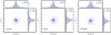 |
Fig. 1 Scatter of the ICRF3 S∕X-band (left), K-band (middle), and X∕Ka-band (right) positions with respect to the Gaia EDR3 positions for the 512 sources in common, after removing relative deformations between these frames. The histograms in the insets at the top and right sides present the distribution of optical-to-radio differences in right ascension and declination before (pre-fit in gray) and after (post-fit in blue) applying the VSH transformation. |
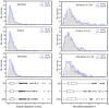 |
Fig. 2 Distributions of optical-to-radio offset ρ (left) and normalized separation X (right) at S∕X-, K-, and X∕Ka-band for the 512 sources in common. The distribution is given for two cases, before (pre-fit in gray) and after (post-fit in blue) applying the VSH transformation. The left and right ends of the box in the boxplot indicate the 25th and 75th percentiles (labeled Q1 and Q3), respectively, and the orange line within the box shows the location of the median value. The ends of the whisker onthe left and right sides show the lower and upper limits of the bulk of the sample, which are Q0 = Q1− 1.5 ×IQR and Q4 = Q3 + 1.5 ×IQR, where IQR = Q3 − Q1. Data points (open circle) greater than Q4 or smaller than Q0 are outliers suggested by the boxplot. There are 50, 53, and 49 such points for S∕X-, K-, and X∕Ka-band, respectively,based on the angular separation; there are 26, 35, and 42 such points based on normalized separation. There are 23 sources at S∕X-band, 8 at K-band, and 12 at X∕Ka-band with X > 10 that are beyond the axis. The dashed red lines in the first three plots on the right represent the Rayleigh distributions with the sigma to be best fit to the sample of sources with X < X0, where X0 = 3.53 (Sect. 4). |
4 Dependence of optical-to-radio offsets on observing frequency
We compared the distribution of optical-to-radio offsets at different radio bands. As shown in Fig. 2, the distributions of the optical-to-radio offset ρ at S∕X-, K-, and X∕Ka-band yield similarshapes, peaking at 0.1–0.2 mas. The number of outliers given by the boxplot, that is, optical-to-radio offsets greater than ~1.2 mas4, is 50, 53, and 49 for S∕X-, K-, and X∕Ka-band, respectively.When the outliers are removed, the 25th, 50th, and 75th percentiles are 0.20 mas, 0.38 mas, and 0.63 mas for the S∕X-band; 0.18 mas, 0.33 mas, and 0.58 mas forthe K-band; and 0.18 mas, 0.34 mas, and 0.61 mas for the X∕Ka-band.
In the right panel in Fig. 2 we plot the distributions of normalized separation X to show the significance of the optical-to-radio offsets. The distributions of X are slightly different from those of ρ: it is sharper for the K-band, but flatter for the S∕X-band. There are 23 sources at S∕X-band, 8 at K-band, and 12 at X∕Ka-band with X > 10 that are beyond the axis. For ideal cases, X is supposed to follow a Rayleigh distribution of unit standard deviation. Medians of normalized separations are 1.89, 1.61, and 1.87 for S∕X-, K-, and X∕Ka-band, respectively,all greater than the predicted median value 1.18 for a standard Rayleigh distribution.
We fitted the normalized separation distributions to the Rayleigh curve with an unknown of standard deviation σ. The fitting returned σ values of 3.29 for S∕X-band, 2.42 for K-band, and 2.62 for X∕Ka-band, indicating that the Gaia-to-S∕X-band offset is more significant than the Gaia-to-K-band and Gaia-to-X∕Ka-band offsets. Considering the bias introduced by the outliers in the fitting, we removed sources with high X values and repeated the fitting. Outliers were identified based on the prediction for a standard Rayleigh distribution. For a sample of N sources with X following a standard Rayleigh distribution, the number of sources with X > X0 is expected to be lower than one when 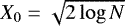 . For our sample (N = 512), X0 is 3.53. This criterion ruled out 115 sources for the S∕X-band, 73 for the K-band, and 93 for the X∕Ka-band. The percentage of outliers for the S∕X-band corresponds to 22% of the sample. Interestingly, this percentage is the same as was found by Charlot et al. (2020) when they compared the ICRF3 S∕X-band frame and the Gaia-CRF2 frame. The standard deviations for the “clean” sample then became 1.29, 1.21, and 1.49 for the S∕X-, K-, and X∕Ka-band, respectively.
We tested whether the optical-to-radio distance decreased at high frequency. For this purpose, we plotted the optical-to-radio offset of individual sources calculated at K-band and X∕Ka-band against that calculated at S∕X-band, and the optical-to-radio offset calculated at X∕Ka-band against that calculated at K-band (Fig. 3). Except for a small fraction (7%), the differences between the optical-to-radio offsets derived from the S∕X- and K-band positions are smaller than 0.5 mas, and the same applies when X∕Ka-band is compared to S∕X-band and X∕Ka-band to K-band. We further performed sign tests between S∕X- and K-band, S∕X- and X∕Ka-band, and K- and X∕Ka-band. The null hypothesis is that the optical-to-radio offset is smaller at high frequency than at low frequency. To assess this hypothesis, we counted the number of sources for which the optical-to-radio offset was smaller at K-band than at S∕X-band, and we repeated this for X∕Ka-band versus S∕X-band and for X∕Ka-band versus K-band. The numbers found in the three cases are 263, 239, and 237, respectively. When we assume that the count follows a binomial random distribution, the corresponding confidence levels to accept the null hypothesis are 75, 7, and 5%. Considering that not all sources in our sample show significant extended structure, we performed the same sign test on the 228 sources that have an X-band structure index greater than 3 (Sect. 5.1). The number of sources for which the high-frequency optical-to-radio offset is smaller than the low-frequency offset is 136 for K versus S∕X, 103 for X∕Ka versus S∕X, and 99 for X∕Ka versus K. These counts correspond to confidence levels of 99.9, 8, and 3% to accept the null hypothesis.
The analysis of the Gaia-to-VLBI offsets allowed us to make three conclusions.
- (i)
The hypothesis that Gaia-to-X∕Ka-band offsets are smaller than Gaia-to-S∕X-band offsets is rejected at a statistical significance level of 93%.
- (ii)
The hypothesis that Gaia-to-K-band offsets are smaller than Gaia-to-S∕X-band offsets is rejected at a statistical significance level of 25%.
- (iii)
The hypothesis that a sample of 228 sources with SI ≥ 3 Gaia-to-K-band offsets are systematically smaller thanGaia-to-S∕X-band offsets is accepted at a statistical significance level of 99.9%.
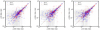 |
Fig. 3 Comparison of optical-to-radio distance at the higher and lower frequencies for 512 sources in common to the ICRF3 and Gaia EDR3 catalogs. Left: K-band vs. S∕X-band. Middle: X∕Ka-band vs. S∕X-band. Right: X∕Ka-band vs. K-band. The blue crosses and red circles distinguish sources with SI values lower than 3 and greater than 3, respectively (SI ≥ 3 suggests an extended structure). |
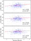 |
Fig. 4 Optical-to-radio offsets at S∕X-, K-, and X∕Ka-band as a function of source structure index for 482 sources. The dashed red line indicates the Nadaraya-Waston estimator for the relation between the optical-to-radio offsets and the structure index. |
5 Correlation of optical-to-radio offsets and source properties
In order to understand the origin of optical-to-radio offsets, we investigated the connection between optical-to-radio offsets and source properties such as the source structure index, G magnitude, redshift, and source type. We first visually checked the correlation using scatter plots, as shown in Figs. 4–6. Then we used the Nadaraya-Waston estimator (Nadaraya 1964; Watson 1964) to empirically characterize the relation between optical-to-radio offsets and source property parameters, as marked by the dashed red lines in these figures. The Nadaraya-Waston estimator can be considered as a local average of the response variable weighted by the kernel (we used the Gaussian kernel here) with the benefit of being independentof the bin width choice (Feigelson & Babu 2012). Finally, we performed the nonparametric Spearman ρS rank test on the data points in these plots to determine the possible connection between quantities. The correlation coefficient ρS and the corresponding p-value are also given therein (the p-value roughly indicates the probability that the null hypothesis is rejected, i.e., that a correlation exists). We considered it to be a genuine correlation when the confidence level given in the correlation test was at least 95%, which means that the p-value should be lower than 0.05. The Kendall τK correlation measure was also computed, which produced consistent results with the Spearman ρS test.
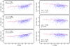 |
Fig. 5 Optical-to-radio offsets (left) and normalized separations (right) at S∕X-, K-, and X∕Ka-band as a functionof the Gaia G magnitude for the 512 sources in our sample. The dashed red line indicates the Nadaraya-Waston estimator for the relation between the optical-to-radio offsets and the G magnitude. |
5.1 Source structure
The structure index at X-band is available for 482 sources (381 directly from BVID and 101 calculated based on Astrogeo images) out of the 512 sources in our sample, most of which (90%) fall in the range of 2–4. A slightly increasing trend is observed at all three bands in Fig. 4, which is more evident at S∕X-band. The Spearman test suggests a correlation of + 0.1 to + 0.2 between optical-to-radio distance and structure index with confidence level of 98% or higher (Table 2), hence indicating a genuine correlation. We also used all the sources in common in the Gaia EDR3 and the ICRF3 catalogs at each band to perform this test and found a similar correlation.
5.2 Magnitude
The source magnitude is available for all 512 sources directly from the Gaia data. Figure 5 demonstrates an obvious dependence of optical-to-radio offsets on the Gaia G magnitude: the optical-to-radio offsets increase toward the faint end for all three radio bands. This correlation is also seen when all sources in common in each ICRF3 individual catalog and Gaia EDR3 catalog are considered. The correlation test further suggests a quite strong correlation (correlation coefficient >+ 0.4) at all three radio bands with a confidence level higher than 99% (Table 2). Considering that the Gaia position uncertainty increases with the magnitude, we also confirmed the correlation between the normalized separation X and the G magnitude. As shown in the right panel of Fig. 5, X decreases with the G magnitude at all three bands; this decreasing tendency is more pronounced at S∕X-band. The negative correlation between normalized separations and the G magnitude is further supported by the results of the correlation tests reported in Table 2. As a check, we repeated these analyses for the Gaia BP (blue photometer covering the wavelength range 330–680 nm) and RP (red photometer covering the wavelength range 640–1050 nm) magnitude and obtained similar results.
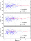 |
Fig. 6 Optical-to-radio offsets at S∕X-, K-, and X∕Ka-band as a functionof the redshift z for 456 sources with a redshift measurement in the LQAC-5 catalog. The dashed red line indicates the Nadaraya-Waston estimator of the relation between the optical-to-radio offsets and the redshift. |
5.3 Redshift
We found redshift measurements in the LQAC-5 catalog for 456 sources, the value of which is between 0.5 and 1.5 for more than half of the sources. For most sources (80%), the redshift is lower than 2. As shown in Fig. 6, there is no indication of a dependence of the optical-to-radio distance on the redshift, which is also supported by results of the correlation tests (see Table 2).
5.4 Source type
We searched for the source type of these sources in the Optical Characteristics of Astrometric Radio Sources catalog (OCARS; Malkin 2018), and found that 355 of them were classified as quasars (labeled “AQ” in the OCARS catalog), while 104 were classified as BL Lac objects (labeled “AL”), and 34 as Seyfert 1 galaxies (labeled “A1”). Then we compared the distribution of the optical-to-radio offsets for the subsets of sources comprised in each class, but did not find any significant difference between the three subsets, meaning that the optical-to-radio offset does not depend on the source type.
6 Discussion
6.1 Cause of the optical-to-radio distance
Petrov & Kovalev (2017a) summarized several causes for the non-coincidence of the emission centers measured by VLBI and Gaia. These include
- (i)
large uncertainties in the Gaia or/and VLBI positions;
- (ii)
optical structure (jet) at the milliarsecond scale;
- (iii)
optical position shift due to a luminous host galaxy or asymmetric structure;
- (iv)
radio source structure and core-shift effect;
- (v)
gravitational lensing and dual AGNs.
We studied these items based on our results, except for the second item, which has been studied deeply in Kovalev et al. (2017, 2020), Petrov & Kovalev (2017a,b), Petrov et al. (2019), and Plavin et al. (2019), and the fifth item, which holds in only very few cases.
Our previous work (Liu et al. 2020) indicated that global deformations between optical and radio catalogs may bias studies of the optical-to-radio offset. Based on the sample of 512 sources in common to the Gaia EDR3 catalog investigated here, we reported a declination bias of approximately − 0.3 mas in the X∕Ka-band positions with respect to the Gaia-EDR3 positions, similar to what was found in the comparison to the Gaia-CRF2 positions. The existence of this declination bias would increase the Gaia-to-X∕Ka-band offset by about 0.1–0.2 mas. For this reason, large-scale systematics in the X∕Ka-band frame should be paid attention. On the other hand, only marginal effects are found for the Gaia-to-S∕X-band offsets or Gaia-to-K-band offsets because the relative deformations between these catalogs are much smaller.
The Gaia position uncertainties increase with the optical G magnitude (Mignard et al. 2016; Gaia Collaboration 2018), while there is no such a dependence for VLBI. We observed that the optical-to-radio offsets increase with G magnitude, especially in the range 17 < G < 21 (Fig. 5). This correlation is further supported by the correlation tests. On the other hand, we also note that the normalized separations between VLBI and Gaia positions generally decrease with G magnitude. A likely explanation is that large optical-to-radio offsets in faint sources are at least partly due to the large Gaia position uncertainties. These large (but not significant) optical-to-radio offsets thus most probably do not have an astrophysical origin.
The radio source structure seen at the lower frequencies might shift the observed position at S∕X-band, while the K- and X∕Ka-band positions would be less affected. If most of the sources had significant structure, the optical-to-radio distance would have statistically decreased at higher frequencies. However, we do not observe such a tendency, nor do we find any statistical evidence in this sense based on our data. Instead, the optical-to-radio offsets in the different bands are roughly at the same level, with the deviation between the bands smaller than 0.5 mas for most sources. On the other hand, when we limit the sample to the sources with SI > 3, that is, sources with extended structures, we find that the optical-to-radio offset is statistically smaller at K-band than that at S∕X-band. This suggests that large optical-to-radio offsets could be a manifestation of extended source structures. This finding was previously reported by Charlot et al. (2020) based on an examination of the structure index for the sources that show significant offsets, as derived from comparing the ICRF3 (S∕X-band) and Gaia-CRF2 positions. As noted above, the X∕Ka-band position is not found to be closer to the optical position than the S∕X- or K-band positions. However, it is difficult to draw firm conclusions on this because of the systematics in the X∕Ka-band frame.
The correlations between the optical-to-radio distances and structure index derived from the X-band VLBI images remain weaker than those between the optical-to-radio distances and the G magnitude (Table 2). To further test this connection, we also examined the structure index measurement at K-band from the BVID, which is available for 224 of our sources. By following the same procedure as described inSect. 5.1, we obtained Spearman correlation coefficients of approximately 0.2 with a confidence level higher than 95%, suggesting again the existence of a correlation between the optical-to-radio distance and structure index. Because no images at Ka-band were available, we were unable to compute SI at this band. We combined the results from correlation tests in the X- and K-bands and found that the optical-to-radio distance correlates positively with the structure index, which also supports that large optical-to-radio offsets could be due to the extended source structure.
Xu et al. (2019) proposed a quantity, namely the closure amplitude root-mean-square (CARMS), to characterize the compactness of the sources based on closure observables. We also studied the correlation between this quantity and optical-to-radio distances using the sample of 464 sources for which it is available. However, we found a lack of connection (correlation coefficient smaller than + 0.1 with a p-value of about 0.4). Because the CARMS was assumed to be correlated with the structure index (Xu et al. 2019) and Xu et al. (2021) reported the existence of a connection between the Gaia-VLBI offset and the CARMS, it is surprising that the correlation tests lead to different results. We have no explanation for this and leave it for a future investigation.
We noted that the LQAC-5 catalog provides optical morphological indices derived from the B, R, and IR Digital Sky Survey (DSS) images, which could be used to infer the existence of a host galaxy. We also computed correlations between morphological indices and optical-to-radio offsets, but no statistically significant correlation was found. Because only a few objects have morphological indices larger than one, the effect of the host galaxy on the Gaia position, if it exists, is not predominant for the bulk of our sample. It is worth noting that these morphological indices were determined from optical imaging with a resolution at the arcsecond level. Thus, they cannot be used to probe the milliarcsecond-scale optical jet. Morphological indices based on high-resolution images might be useful to probe the existence of the milliarcsecond-scale optical jets suggested by Petrov & Kovalev (2017b).
Makarov et al. (2017) found that the optical-to-radio distance at S∕X-band decreases rapidly with redshift z up to z < 0.5. They inferred that the shift of the Gaia positions due to extended optical structures partly explains this finding, noting that the corresponding effect becomes smaller for distant sources. Our sample does not support this explanation. However, the number of sources located at z < 0.5 in our sample is limited, preventing us from drawing any firm conclusion about it.
Previous studies based on ground-based optical observations also investigated the correlation between the optical-to-radio offset and source properties. However, they obtained inconsistent results. Camargo et al. (2011), and Zacharias & Zacharias (2014) reported that the optical-to-radio offset increases with the structure index, while Assafin et al. (2013) did not detect any dependence. Zacharias & Zacharias (2014) found a negative correlation between the optical-to-radio offset and the redshift, but this relation was not found in Orosz & Frey (2013). To further investigate this matter, we cross-matched their catalogs with the Gaia EDR3. When we use the Gaia positions instead, we easily find that the optical-to-radio offsets as large as 20–40 mas reported in Assafin et al. (2013) and Zacharias & Zacharias (2014) largely vanish and turn into values that are mostly lower than 1 mas with Gaia. Mignard et al. (2016) reported similar results based on a comparison of the optical-to-radio offsets from the Gaia DR1 with those from Zacharias & Zacharias (2014). Most likely, these large optical-to-radio offsets only reveal artifacts that are due to unaccounted-for errors in ground-based optical astrometry.
Spearman correlation coefficients between the optical-to-radio offsets and source properties for our sample of 512 sources.
6.2 Implication for the alignment of the optical and radio frames
One reason to extend the ICRF to the K- and X∕Ka-band is that VLBI observations at high frequencies are probably less strongly affected by the radio source structure. Another reason is that the VLBI core at high frequency may be located closer to the optically emitting center, making the K- and X∕Ka-band frames perhaps more suitable for the radio-optical frame alignment (e.g., Jacobs et al. 2002). We found evidence that supports the hypothesis that the K-to-Gaia position offset is statistically smaller thanthe S∕X-to-Gaia offset for one-third of the sources in our sample, namely those that show extended structures. However, when we consider all sources in common, the K-to-Gaia and X∕Ka-to-Gaia offsets are found not to be smaller than the S∕X-to-Gaia offset. As shown here and in our previous study (Liu et al. 2020), the overall agreement between the ICRF3 K- and X∕Ka-band catalogs and the Gaia EDR3 solution remains no higher than for the ICRF3 S∕X-band catalog. In addition, the sample of sources in common with Gaia in the ICRF3 K- and X∕Ka-band catalogs is also much smaller. These factors suggest that the K- and X∕Ka-band frames are currently not a better choice for the alignment of the optical and radio frames than the S∕X-band frame.
Previous authors (Bourda et al. 2008; Makarov et al. 2012) suggested basing the optical-to-radio frame alignment on sources that have no extended radio structures and are optically bright (e.g., with magnitude <18), in other words, have a high astrometric accuracy on both the VLBI and Gaia sides. In this respect, we detected a connection between the optical-to-radio offset and the source structure index, justifying that the SI is a good indicator for the relevant source selection. We also found a strong negative correlation between the optical-to-radio offsets and the Gaia G magnitude at all three radio bands. This correlation is likely caused by the increased Gaia positional uncertainty at the faint end. As a result, the large optical-to-radio offsets for faint sources are often not statistically significant when their uncertainties are considered, meaning that these offsets most probably are not linked to source properties such as extended radio structures or core-shift effects (e.g., Kovalev et al. 2008; Porcas 2009). In this case, including faint sources in the sample of sources used for the alignment probably only adds random noise. On the other hand, it will greatly enlarge the sample of sources in common between radio and optical. Liu et al. (2020) found that the accuracy of the Gaia-CRF2 alignment did not degrade when the magnitude limit of the sample was increased. The objects for the alignment between the Gaia-CRF and the ICRF may therefore not have to be optically bright.
7 Conclusions
For the first time, we achieved a multifrequency comparison of extragalactic source positions targeted to study the frequency dependence of those positions. To this end, we used a sample of 512 extragalactic sources with positions in the S∕X, K, and X∕Ka radio bands available in ICRF3 and with the optical positions known from the Gaia EDR3 catalog. Our main findings are listed below.
The large-scale systematics in the ICRF3 X∕Ka-band catalog distorts the optical-radio vector. When this is unaccounted for, these systematic errors increase the optical-radio distance by 0.1–0.2 mas on average.
The differences between Gaia-to-S∕X-band, Gaia-to-K-band, and Gaia-to-X∕Ka-band position offsets is statistically insignificant for the entire sample of 512 sources we investigated.
However, the Gaia-to-K-band distance is shorter than that of the Gaia-to-S∕X-band for a subsample of 228 sources with structure index >3. This result is statistically significant at the 99% level.
The correlation coefficient between the optical-radio distance and the structure index is in the range of 0.12–0.18. This correlation is statistically significant at the 98% level.
The optical-radio distance increases with the Gaia G magnitude, but shows a generally decreasing trend when normalized by the uncertainty.
Based on our results, the ICRF3 S∕X-band frame remains the preferred choice for aligning the Gaia-CRF to the ICRF because (i) it has smaller systematics, (ii) it has more sources in common to Gaia catalogs, and (iii) the Gaia-to-X∕Ka and Gaia-to-K offsets are not statistically smaller thanthe Gaia-to-S∕X offsets when all sources in our sample are considered. The efforts to improve the K- and X∕Ka-band frames should be continued, which should help to further assess the dependence of optical-to-radio distance on source structure, magnitude, and redshift.
Acknowledgements
We sincerely thank the anonymous referee for the constructive comments and useful suggestions, which improved the work significantly. N.L. and Z.Z. are supported by the National Natural Science Foundation of China (NSFC) under grant No. 11833004. N.L. is also supported by the Fundamental Research Funds for the Central Universities of China (grant No. 14380042) and China Postdoctoral Science Foundation (grant No. 2021M691530). This work has made use of data from the European Space Agency (ESA) mission Gaia (https://www.cosmos.esa.int/gaia), processed by the Gaia Data Processing and Analysis Consortium (DPAC, https://www.cosmos.esa.int/web/gaia/dpac/consortium). Funding for the DPAC has been provided by national institutions, in particular the institutions participating in the Gaia Multilateral Agreement. This research has made use of material from the Bordeaux VLBI Image Database (BVID). This database can be reached at http://bvid.astrophy.u-bordeaux.fr/. Some radio images were retrieved from the Astrogeo VLBI FITS image database (http://astrogeo.org/vlbi_images/). This research had also made use of Astropy (http://www.astropy.org) – a community-developed core Python package for Astronomy (Astropy Collaboration 2018), the Python 2D plotting library Matplotlib (Hunter 2007), and TOPCAT (Taylor 2011). We made much use of NASA’s Astrophysics Data System and the VizieR catalogue access tool, CDS, Strasbourg, France (DOI : 10.26093/cds/vizier). The original description of the VizieR service was published in Ochsenbein et al. (2000).
References
- Aslan, Z., Gumerov, R., Jin, W., et al. 2010, A&A, 510, A10 [NASA ADS] [CrossRef] [EDP Sciences] [Google Scholar]
- Assafin, M., Vieira-Martins, R., Andrei, A. H., Camargo, J. I. B., & da Silva Neto, D. N. 2013, MNRAS, 430, 2797 [NASA ADS] [CrossRef] [Google Scholar]
- Astropy Collaboration (Price-Whelan, A. M., et al.) 2018, AJ, 156, 123 [Google Scholar]
- Bourda, G., Charlot, P., & Le Campion, J. F. 2008, A&A, 490, 403 [NASA ADS] [CrossRef] [EDP Sciences] [Google Scholar]
- Camargo, J. I. B., Andrei, A. H., Assafin, M., Vieira-Martins, R., & da Silva Neto, D. N. 2011, A&A, 532, A115 [NASA ADS] [CrossRef] [EDP Sciences] [Google Scholar]
- Charlot, P., Boboltz, D. A., Fey, A. L., et al. 2010, AJ, 139, 1713 [NASA ADS] [CrossRef] [Google Scholar]
- Charlot, P., Jacobs, C. S., Gordon, D., et al. 2020, A&A, 644, A159 [EDP Sciences] [Google Scholar]
- Feigelson, E. D., & Babu, G. J. 2012, Modern Statistical Methods for Astronomy (Cambridge: Cambridge University Press) [Google Scholar]
- Fey, A. L., & Charlot, P. 1997, ApJS, 111, 95 [NASA ADS] [CrossRef] [Google Scholar]
- Fey, A. L., Gordon, D., Jacobs, C. S., et al. 2015, AJ, 150, 58 [Google Scholar]
- Frouard, J., Johnson, M. C., Fey, A., Makarov, V. V., & Dorland, B. N. 2018, AJ, 155, 229 [Google Scholar]
- Gaia Collaboration (Prusti, T., et al.) 2016, A&A, 595, A1 [NASA ADS] [CrossRef] [EDP Sciences] [Google Scholar]
- Gaia Collaboration (Mignard, F., et al.) 2018, A&A, 616, A14 [NASA ADS] [CrossRef] [EDP Sciences] [Google Scholar]
- Gaia Collaboration (Brown, A. G. A., et al.) 2021, A&A, 649, A1 [NASA ADS] [CrossRef] [EDP Sciences] [Google Scholar]
- Hunter, J. D. 2007, Comput. Sci. Eng., 9, 90 [NASA ADS] [CrossRef] [Google Scholar]
- Jacobs, C. S., Jones, D. L., Lanyi, G. E., et al. 2002, in International VLBI Service for Geodesy and Astrometry: General Meeting Proceedings, ed. N. R. Vandenberg, & K. D. Baver, 350 [Google Scholar]
- Kovalev, Y. Y., Lobanov, A. P., Pushkarev, A. B., & Zensus, J. A. 2008, A&A, 483, 759 [NASA ADS] [CrossRef] [EDP Sciences] [Google Scholar]
- Kovalev, Y. Y., Petrov, L., & Plavin, A. V. 2017, A&A, 598, L1 [NASA ADS] [CrossRef] [EDP Sciences] [Google Scholar]
- Kovalev, Y. Y., Zobnina, D. I., Plavin, A. V., & Blinov, D. 2020, MNRAS, 493, L54 [NASA ADS] [CrossRef] [Google Scholar]
- Liu, N., Lambert, S. B., Zhu, Z., & Liu, J. C. 2020, A&A, 634, A28 [EDP Sciences] [Google Scholar]
- Makarov, V., Berghea, C., Boboltz, D., et al. 2012, Mem. Soc. Astron. It., 83, 952 [Google Scholar]
- Makarov, V. V., Frouard, J., Berghea, C. T., et al. 2017, ApJ, 835, L30 [Google Scholar]
- Makarov, V. V., Berghea, C. T., Frouard, J., Fey, A., & Schmitt, H. R. 2019, ApJ, 873, 132 [NASA ADS] [CrossRef] [Google Scholar]
- Malkin, Z. 2018, ApJS, 239, 20 [CrossRef] [Google Scholar]
- Mignard, F., & Klioner, S. 2012, A&A, 547, A59 [NASA ADS] [CrossRef] [EDP Sciences] [Google Scholar]
- Mignard, F., Klioner, S., Lindegren, L., et al. 2016, A&A, 595, A5 [NASA ADS] [CrossRef] [EDP Sciences] [Google Scholar]
- Nadaraya, E. A. 1964, Theor. Probabi. Appl., 9, 141 [Google Scholar]
- Ochsenbein, F., Bauer, P., & Marcout, J. 2000, A&AS, 143, 23 [NASA ADS] [CrossRef] [EDP Sciences] [Google Scholar]
- Orosz, G., & Frey, S. 2013, A&A, 553, A13 [NASA ADS] [CrossRef] [EDP Sciences] [Google Scholar]
- Petrov, L., & Kovalev, Y. Y. 2017a, MNRAS, 471, 3775 [NASA ADS] [CrossRef] [Google Scholar]
- Petrov, L., & Kovalev, Y. Y. 2017b, MNRAS, 467, L71 [Google Scholar]
- Petrov, L., Kovalev, Y. Y., & Plavin, A. V. 2019, MNRAS, 482, 3023 [NASA ADS] [CrossRef] [Google Scholar]
- Plavin, A. V., Kovalev, Y. Y., & Petrov, L. Y. 2019, ApJ, 871, 143 [NASA ADS] [CrossRef] [Google Scholar]
- Porcas, R. W. 2009, A&A, 505, L1 [NASA ADS] [CrossRef] [EDP Sciences] [Google Scholar]
- Shabala, S. S., Rogers, J. G., McCallum, J. N., et al. 2014, J. Geodesy, 88, 575 [Google Scholar]
- Souchay, J., Gattano, C., Andrei, A. H., et al. 2019, A&A, 624, A145 [EDP Sciences] [Google Scholar]
- Taylor, M. 2011, TOPCAT: Tool for OPerations on Catalogues And Tables [Google Scholar]
- Watson, G. S. 1964, Sankhyā: Indian J. Stat. Ser. A, 26, 359 [Google Scholar]
- Xu, M. H., Anderson, J. M., Heinkelmann, R., et al. 2019, ApJS, 242, 5 [NASA ADS] [CrossRef] [Google Scholar]
- Xu, M. H., Lunz, S., Anderson, J. M., et al. 2021, A&A, 647, A189 [EDP Sciences] [Google Scholar]
- Zacharias, N., & Zacharias, M. I. 2014, AJ, 147, 95 [NASA ADS] [CrossRef] [Google Scholar]
In the boxplot, the interquartile range (IQR) is defined as the distance between the 25th percentile (Q1) and 75th percentile (Q3), i.e., IQR = Q3 − Q1. Data points smaller than Q0 = Q1 − 1.5 ×IQR or greater than Q4 = Q3 + 1.5 ×IQR are considered as outliers. Because there are no outliers (open circles) on the left side of the boxplots in Fig. 2, we exclusively considered the upper limit Q4, which is about 1.2 mas.
All Tables
Median formal uncertainties for 512 common sources in the ICRF3 (S∕X-, K-, and X∕Ka-band) and Gaia EDR3 catalogs.
Spearman correlation coefficients between the optical-to-radio offsets and source properties for our sample of 512 sources.
All Figures
|
Fig. 1 Scatter of the ICRF3 S∕X-band (left), K-band (middle), and X∕Ka-band (right) positions with respect to the Gaia EDR3 positions for the 512 sources in common, after removing relative deformations between these frames. The histograms in the insets at the top and right sides present the distribution of optical-to-radio differences in right ascension and declination before (pre-fit in gray) and after (post-fit in blue) applying the VSH transformation. |
| In the text | |
|
Fig. 2 Distributions of optical-to-radio offset ρ (left) and normalized separation X (right) at S∕X-, K-, and X∕Ka-band for the 512 sources in common. The distribution is given for two cases, before (pre-fit in gray) and after (post-fit in blue) applying the VSH transformation. The left and right ends of the box in the boxplot indicate the 25th and 75th percentiles (labeled Q1 and Q3), respectively, and the orange line within the box shows the location of the median value. The ends of the whisker onthe left and right sides show the lower and upper limits of the bulk of the sample, which are Q0 = Q1− 1.5 ×IQR and Q4 = Q3 + 1.5 ×IQR, where IQR = Q3 − Q1. Data points (open circle) greater than Q4 or smaller than Q0 are outliers suggested by the boxplot. There are 50, 53, and 49 such points for S∕X-, K-, and X∕Ka-band, respectively,based on the angular separation; there are 26, 35, and 42 such points based on normalized separation. There are 23 sources at S∕X-band, 8 at K-band, and 12 at X∕Ka-band with X > 10 that are beyond the axis. The dashed red lines in the first three plots on the right represent the Rayleigh distributions with the sigma to be best fit to the sample of sources with X < X0, where X0 = 3.53 (Sect. 4). |
| In the text | |
|
Fig. 3 Comparison of optical-to-radio distance at the higher and lower frequencies for 512 sources in common to the ICRF3 and Gaia EDR3 catalogs. Left: K-band vs. S∕X-band. Middle: X∕Ka-band vs. S∕X-band. Right: X∕Ka-band vs. K-band. The blue crosses and red circles distinguish sources with SI values lower than 3 and greater than 3, respectively (SI ≥ 3 suggests an extended structure). |
| In the text | |
|
Fig. 4 Optical-to-radio offsets at S∕X-, K-, and X∕Ka-band as a function of source structure index for 482 sources. The dashed red line indicates the Nadaraya-Waston estimator for the relation between the optical-to-radio offsets and the structure index. |
| In the text | |
|
Fig. 5 Optical-to-radio offsets (left) and normalized separations (right) at S∕X-, K-, and X∕Ka-band as a functionof the Gaia G magnitude for the 512 sources in our sample. The dashed red line indicates the Nadaraya-Waston estimator for the relation between the optical-to-radio offsets and the G magnitude. |
| In the text | |
|
Fig. 6 Optical-to-radio offsets at S∕X-, K-, and X∕Ka-band as a functionof the redshift z for 456 sources with a redshift measurement in the LQAC-5 catalog. The dashed red line indicates the Nadaraya-Waston estimator of the relation between the optical-to-radio offsets and the redshift. |
| In the text | |
Current usage metrics show cumulative count of Article Views (full-text article views including HTML views, PDF and ePub downloads, according to the available data) and Abstracts Views on Vision4Press platform.
Data correspond to usage on the plateform after 2015. The current usage metrics is available 48-96 hours after online publication and is updated daily on week days.
Initial download of the metrics may take a while.