| Issue |
A&A
Volume 651, July 2021
|
|
|---|---|---|
| Article Number | A64 | |
| Number of page(s) | 7 | |
| Section | Extragalactic astronomy | |
| DOI | https://doi.org/10.1051/0004-6361/202140652 | |
| Published online | 13 July 2021 | |
Parsec-scale alignments of radio-optical offsets with jets in AGNs from multifrequency geodetic VLBI, Gaia EDR3, and the MOJAVE program⋆
1
SYRTE, Observatoire de Paris – Université PSL, CNRS, Sorbonne Université, LNE, Paris, France
e-mail: This email address is being protected from spambots. You need JavaScript enabled to view it.
2
School of Astronomy and Space Science, Key Laboratory of Modern Astronomy and Astrophysics (Ministry of Education), Nanjing University, Nanjing, PR China
Received:
24
February
2021
Accepted:
29
April
2021
Abstract
Aims. We aim to study the relative positions of quasar emission centers at different wavelengths in order to help link the various realizations of the International Celestial Reference System (ICRS), and to unveil systematic uncertainties and individual source behavior at different wavelengths.
Methods. We based our study on four catalogs representing the ICRS, the ICRF3 positions in the three VLBI bands X, K, and Ka, and the Gaia EDR3 catalog in optical wavelengths. We complemented radio source positions with jet kinematics results from the MOJAVE team, allowing us to obtain jet directions on the sky. A six-parameter deformation model was used to remove systematic uncertainties present in the different catalogs.
Results. For a set of 194 objects common to the four catalogs and to the objects whose jet kinematics was studied by the MOJAVE team, we computed the orientation between positions at the different wavelengths and with respect to the directions of the jets. We find that the majority of these objects have their radio-to-optical vector along the jet, with the optical centroid downstream from the radio centroids, and that the K and Ka centroids are preferably upstream in the jet with respect to the X centroid, which is consistent with the paradigm of a simple core–jet model. For a population of multiwavelength positions aligned along the jet, astrometric information can therefore be used to measure the direction of the jet independently of imaging. In addition, we find several sources for which the optical centroid coincides with stationary radio features with a relatively high fraction of polarization, indicating optical emission dominated by a synchrotron process in the jet.
Key words: reference systems / astrometry / galaxies: jets / techniques: interferometric
Table A.1 is only available at the CDS via anonymous ftp to cdsarc.u-strasbg.fr (130.79.128.5) or via http://cdsarc.u-strasbg.fr/viz-bin/cat/J/A+A/651/A64
© S. Lambert et al. 2021
 Open Access article, published by EDP Sciences, under the terms of the Creative Commons Attribution License (https://creativecommons.org/licenses/by/4.0), which permits unrestricted use, distribution, and reproduction in any medium, provided the original work is properly cited.
1. Introduction
On 2020 December 13, the Early Data Release 3 (EDR3) of the Gaia mission (Prusti et al. 2016; Brown et al. 2021) provided a new astrometric solution in the optical domain for more than 1.8billion celestial objects. Among them are roughly one and half million active galactic nuclei (AGNs) or quasars that can be identified through a cross match with specific ground-based catalogs. The most recent realization of the International Celestial Reference Frame (ICRF3, Charlot et al. 2020) was based on 30 years of very long baseline interferometry (VLBI) observations and consists of equatorial coordinates for a set of about 4800 AGNs and quasars whose positions are given, for hundreds of them, at three frequency bands. These four catalogs meet the requirements of the International Celestial Reference System (ICRS, Arias et al. 1995) and are aligned to each other thanks to a set of common sources in the optical and radio bands. Moreover, the objects common to the catalogs exhibit a comparable median positional accuracy of less than 0.2 milliarcsec (mas) and constitute the current best realizations of the ICRS.
Studying the relative positions of emission centers at different wavelengths is a crucial step in the context of linking the various realizations of the ICRS and unveiling general trends and individual source particularities in multifrequency signatures of core-shift, accretion disks, and host galaxies. Several studies were carried out in that context that reported the existence of the optical jet at milliarcsecond scale and that the radio-to-optical vector favors the jet direction (Makarov et al. 2017; Kovalev et al. 2017; Frouard et al. 2018; Petrov et al. 2018). However, these works are limited to one radio frequency. In the present study, we make use of three radio frequencies of the ICRF3 catalog together with the Gaia EDR3 sample – amounting to four different positions – and the jet directions from the most recent fitting of jet kinematics from the Monitoring of Jets in Active Galactic Nuclei with VLBA Experiments (MOJAVE) sample by Lister et al. (2019). Here, we aim to check the alignments mentioned above for more than one radio frequency and to compare the results with the scenario of the core–jet model in which the optical emitting center is almost collocated with the central engine of the AGN while the radio emitting center is located, depending on the observing frequency, downstream of the jet.
2. Data and their preparation
Our radio catalog is the ICRF31 (Charlot et al. 2020). It includes the positions of 4588 extragalactic radiosources, of which 4536 are observed at 8.4 GHz and 600 are observed in three frequencies (X-band: 8.4 GHz, K-band: 24 GHz, and Ka-band: 32 GHz). In the following, for brevity, the positions of the centroids at different wavelengths will be designated by the band name only. For the optical counterparts, we proceeded with a cross-matching of the full Gaia EDR32 positions (Prusti et al. 2016; Brown et al. 2021) with the ICRF3 positions at X-band with a cross-identification radius of 0.1 mas. We find 3477sources. None of these have statistically significant parallaxes. For simplification, we use O (for “optical”) to refer to the Gaia EDR3 positions. There are 544 sources for which the four X, K, Ka, and O positions are available.
Lister et al. (2019) used very long baseline array (VLBA) maps of 409 radio-loud blazars acquired in the framework of the MOJAVE survey at 15.4 GHz between 1994 and 2016. Of these sources, 194 are common to the 544 sources found in common between ICRF3 and Gaia EDR3. Tracking the relative positions of bright, parsec-scale (i.e., mas-scale) features, they provide the time-dependent coordinates and fluxes of VLBI components relative to a putative core component (region close to the apparent base of the jet with an optical depth close to 1 at a given frequency) at several epochs. We used this information (Table 1 of Lister et al. 2019) to measure a jet direction on the sky. For each source, the jet position angle with respect to the stationary component was computed as the time-integrated flux-weighted average of the positions of all nonstationary components at all epochs. Uncertainties on position angles were computed as the time-integrated flux-weighted standard deviation of the positions. We did not consider time-variation of the jet direction, or, more specifically, we considered it as included in the uncertainty.
The presence of large-scale systematic errors in all four catalogs could bias the study, especially as the weaknesses and/or north–south asymmetry in some VLBI networks induces a declination-dependent positional error in catalogs (Charlot et al. 2020). To remove these systematic errors as efficiently as possible, we modeled the coordinate differences between the X-band catalog of the other catalogs as a six-parameter transformation made up of three rotations around the X, Y, and Z axes of the ICRS, and a glide (e.g., Mignard & Klioner 2012). The parameters were adjusted to the coordinate differences for the 544 sources common to ICRF3 and Gaia EDR3 with a weighting method that includes the correlation between right ascension and declination and an outlier removal before adjustment as described in (Charlot et al. 2020). No significant glide was detected between EDR3, X, and K samples. However, a deformation in sin δ of −0.30 ± 0.01 mas in amplitude was found between X and Ka. We note that the Ka catalog was obtained with a VLBI network of only four sites. This limited geometry, lacking north–south baselines, is likely at the origin of the observed deformation. After removal of this systematic error, residual transformation parameters are not zero but are nevertheless reduced by an order of magnitude, resulting in only a small persistent systematic error in sin δ between X and Ka catalogs (0.03 ± 0.01 mas) whose impact on the distributions of position angles can be seen in the left panels of Fig. 1. We take into account these errors when assessing the significance of the distributions studied further below.
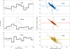 |
Fig. 1. Left: orientation of the X-to-K, X-to-Ka, and X-to-O vectors for the 194 sources used for the comparison before (thin line) and after (thick line) adjustment of large-scale systematic errors measured relative to the north, turning positive into the direction of right ascension. Right: uncertainty on the position angles versus the angular separation. The vertical (horizontal) lines represent the median values of the angular separations (position angle uncertainties) for each frequency. |
The final material for this study is therefore made up of the differences X-to-K, X-to-Ka, and X-to-O – after removal of estimated systematic errors – expressed as arc length and position angle, with their respective uncertainties, and of the jet position angles with their uncertainties, for 194 sources. This material is displayed in Table A.1 of Appendix A.
3. Analysis and results
The right panels of Fig. 1 show the position angle uncertainty as a function of the distance to the X centroid, revealing that at short distances, where error ellipses possibly overlap, the angles are generally not precisely determined. The median uncertainties on the position angles are 21°, 27°, and 45° for X-to-O, X-to-Ka, and X-to-K, respectively. Corresponding median separations are 0.333 mas, 0.192 mas, and 0.107 mas, respectively. Figure 2 displays the positions of K, Ka, and O centroids relative to the X centroid (located at coordinates (0,0) in the figure) and decomposed along and perpendicularly to the direction of the jet (i.e., along the x-axis of the plot). We fitted two-dimensional Gaussian distributions to the cloud points and reported the contour of 99% confidence ellipses (three times the standard deviation of the Gaussian distributions). The bottom panel of the figure displays the loci of the median position for each wavelength: these are −0.013 ± 0.001 mas, −0.028 ± 0.006 mas, and 0.173 ± 0.035 mas for K, Ka, and O, respectively. (The 1σ uncertainties on the median are computed using the weighted standard deviation.) We note that (i) the three radio centroids are close to each other within a few tens of microarcseconds, whereas the optical centroid is generally farther by a factor of ten and (ii) the optical centroid is upstream in the jet with respect to the X centroid, whereas the K and Ka centroids appear to be downstream.
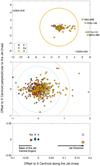 |
Fig. 2. Top: positions of K (diamonds), Ka (squares), and O (discs) centroids relative to the X centroid and decomposed along and perpendicularly to the jet direction. The ellipses represent the contour of 99% confidence for the K (dashed line), KA (thin line), and O (thick line) point clouds. Middle: same as above but zoomed. Bottom: loci of the median position for each wavelength with X conventionally set at (0,0). |
In the case of a self-absorbed core and equipartition between jet particle and magnetic field energy density, the absolute distance of the core from the central engine is inversely proportional to the observing frequency (Blandford & Königl 1979; Konigl 1981; Lobanov 1998; Pushkarev et al. 2012). It turns out that, for two different observing frequencies ν1 and ν2 (ν2 > ν1), the position of the radio core appears shifted from the core along the jet proportionally to (ν2 − ν1)/ν1ν2. For frequencies K, Ka, and O, one expects centroids to be closer to the base of the jet than for X and thereby shifted to the left in Fig. 2 (the base of the jet is therefore left of Ka). However, assuming this model, the optical centroid should have been left of Ka. This suggests that the optical centroid results from the combination of several optical features, including emission from one or several ejected components, but also from the accretion disk or a host galaxy. The ratio of X-to-K to X-to-Ka distances along the jet expected from the core-shift model is 1.2. This values is shown as a red line in Fig. 3 which shows all individual X-to-K and X-to-Ka distances as projected along the jet. The ratio of the median X-to-K and X-to-Ka distances is 2.3 ± 0.7 which includes the theoretical ratio within 2σ. We note that the observed (individual or median) values could be vitiated by unaccounted errors – especially in the Ka positions – due to the systematic uncertainties discussed in the previous section.
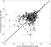 |
Fig. 3. X-to-Ka distance versus X-to-Ka distance for all 194 sources. The diagonal thick line represents the distance expected for the core-shift model, i.e., 1.2 (see text). |
We made composite maps of intensity distribution together with X, K, Ka, and O positions for the 194 sources common to MOJAVE, ICRF3, and Gaia EDR33. The intensity distribution was obtained from the stacking of all components provided by Lister et al. (2019) convoluted by a Gaussian circular beam of radius 0.1 mas. For better visualization, we set the X centroid onto the stationary component of Lister et al. (2019). Doing so, we do not account for the core-shift effect between 8.4 and 15.4 GHz which is of the order of 0.1–0.3 mas following dedicated measurements by Pushkarev et al. (2012) and is expected to be along the jet direction. This omission is unlikely to affect the conclusion of this study concerning the jet direction, which is determined over the structure only. The error ellipses in the maps represent three times the error ellipse deduced from uncertainties in right ascension and declination and their correlations as reported in the ICRF3 and Gaia EDR3 catalogs.
Some of these maps are shown in Fig. 4 either because of a particularly large and significant radio-to-optical distance (the sources out of the 99% ellipse in Fig. 2) or because we found by visual inspection that the optical centroid falls onto or close to a detected radio component. Two sources (0003+380, 0250+320) among the six “outliers” of Fig. 2 present a kiloparsec-scale (arcsecond-scale) radio morphology of an unresolved core component only (Lister et al. 2019). The other four sources (0119+115, 1538+149, 1652+398, and 2353+816) show emission on one side of an unresolved core component (Taylor et al. 1996; Cassaro et al. 1999; Cooper et al. 2007). Two sources (1538+149 and 2353+816) presenting particularly large X-to-O offsets are also ICRF3 defining sources. In several sources (0119+115, 0346+800, 0749+540, 0859+470, 1157−215, 1652+398, 1742−078, and 2223−052), the optical centroid is close to a radio jet feature (a particularity also recently supported by Xu et al. 2021), suggesting that in such sources the optical emission is dominated by optically thin jet features in the downstream region of the jet. Such regions of synchrotron emission are expected to have a more organized magnetic field and higher linear polarization (e.g., Ginzburg 1979), which is supported by observations in radio Lister & Homan (2005) and optical Kovalev et al. (2020). More comments on the above-cited sources are reported in Appendix B. Although a source-per-source examination of all radio-optical links is out of the scope of this paper, brief inspection of the MOJAVE data for these 12 sources suggests that, when the optical centroid can be identified with a radio feature in the jet (0346+800, 0749+540, 1652+398, 1742−078, 2223−052), the latter is a quasi-stationary component with a substantial fractional polarization. These results should encourage the MOJAVE team to pursue the regular follow-up of AGNs, including the measurement of radio polarization when possible.
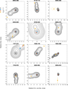 |
Fig. 4. Maps reconstructed from MOJAVE modelfitting of Lister et al. (2019) with X, K, Ka, and O centroids for particular sources (see text) and their 99% confidence ellipses. |
To check the alignment of the four centroids and the jets, we computed the angles between X-to-K, X-to-Ka, and X-to-O vectors and the jet, taking the origin at X. Hereafter, an angle named A-B-C refers to the angle between the vectors B-to-A and B-to-C, with B at the vertex. The distributions of the angles are shown in Fig. 5 where we used bins of 30°. Though a peak is clearly showing up at 0 degrees in the bottom panel (O-X-Jet) suggesting that the optical and X centroids are aligned in the direction of the jet, consistently with Kovalev et al. (2017) and Petrov et al. (2018), there is much more uncertainty regarding the alignment of X-to-K and X-to-Ka versus the jet. We wanted to test the statistical significance of the distribution. The null hypothesis is that the obtained distributions result from the difference of two random distributions of position angles that nevertheless still contain the systematic errors evidenced in Fig. 1. To test the null hypothesis, we considered randomly redistributing the X-to-K, X-to-Ka, and X-to-O position angles by uniform random permutation of indices and reforming their differences. The procedure was repeated 1000 times, resulting in 1000 distributions from which we could derive a mean distribution and its standard deviation. These are illustrated in Fig. 5 by the thin blue lines: the solid line represents the mean and the two dashed lines represent three standard deviations around the mean. We computed a z-score for the histogram peak as the number of standard deviations by which the peak height differs from the mean. We derived a p-value from the z-score, giving the probability that the null hypothesis is verified (reported in blue on the right side of the histogram plots). We also tested how the uncertainties on position angles could affect the histogram by forming 1000 replicas of the sets of position angles, each angle being randomly perturbed by a Gaussian error of sigma, that is, the standard error of the position angles. Similarly to the previous test, we formed a mean histogram and a confidence interval, which are shown by the thick red curves in Fig. 5. Corresponding z-scores and p-values for the peaks are given in bold red characters on the left side of the histogram plots.
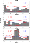 |
Fig. 5. Relative orientation of the jet and of the vectors X-to-K, X-to-Ka, and X-to-O. The area between the thin dashed blue lines represents the 99% confidence interval based on random permutations of the input series. The z-score and p-value are reported on the right side of the axis box. The area between the thick dashed red lines represents the 99% confidence interval based on a bootstrap of the input series modified by a Gaussian error corresponding to their standard error. The z-score and p-value are reported on the left side of the axis box. |
In light of these tests, the K-X-Jet and Ka-X-Jet triads show insignificant (or very weakly significant) peaks at 0°. The significant peak at 180° in K-X-Jet, suggesting that the K centroid is downstream in the jet relative to X, is consistent with Fig. 2. As mentioned earlier, the plot for O-X-Jet shows that the optical centroid is located towards the external side of the jet (on the opposite side of the jet base). We tested how the peak significance depends on the radio-to-optical distance. We formed quantiles of the X-to-O values at five evenly spaced cumulative probabilities between 0 and 1. For each quantile, we considered the sources distributed in the bins immediately on the left and on the right. Therefore, we obtained five overlapping bins each containing about 55 sources. We then computed the histogram of the distribution of the O-X-Jet angles in each bin, the z-score of their central peak, and the median uncertainty of the X-to-O position angles. These quantities are represented in Fig. 6 as a function of the quantile. The general trend is a z-score increasing with radio-to-optical distance, showing that the significance of the peak is constrained by sources with large X-to-O distance. The conclusion is robust if we consider a different number of quantiles, as long as the number of sources in each bin remains reasonable.
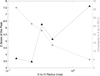 |
Fig. 6. Black triangles, dashed line, left y-scale: significance of the O-X-jet histogram peak as a function of X-to-O distance. Gray stars, solid line, right y-scale: median uncertainty on the X-to-O position angle as a function of X-to-O distance. |
4. Conclusion
This study compares, for the first time, absolute astrometry positions at four frequencies (VLBI radio bands at 8.4, 24, and 32 GHz and optical Gaia EDR3 data) with parsec-scale relativistic jet directions (from 15.4 GHz VLBA observations of the MOJAVE program) for 194 extragalactic radio sources. Our results confirm the finding of Kovalev et al. (2017) that, with respect to the X centroid, the optical centroid is downstream in the jet, especially when the radio-to-optical distance is large. Conclusions about the alignment between the three radio positions and the jet are more elusive because of the relatively high uncertainties (compared with the angular separation) in X-to-K and X-to-Ka directions. With respect to the X centroid, Ka and K centroids appear shifted towards the jet base, which is consistent with the paradigm of a simple core–jet model in which the core-shift effect shifts the centroid away from the base of the jet as observing frequency increases. These results imply that for a population of aligned multiwavelength positions, the astrometry information alone can provide a measurement for the jet direction, independently of the imaging. We note that the orientation of the multiwavelength position vector, as well as the multiwavelength position alignment, might be strongly biased by the systematic errors in the catalogs. Our results also justify that the ICRF3 X-band frame is accurate and reliable.
Another finding of this study is the presence of several sources for which the optical centroid coincides with stationary radio features with relatively high fractional polarization, indicating that the optical emission detected by Gaia is dominated by synchrotron emission within the downstream jet. For theses sources, although the geodetic VLBI position is relevant to the region closer to the core, the optical location is nevertheless accessible in radio.
A deeper exploitation of the multiwavelength data would require an increase in precision and i the accuracy of K and Ka reference frames, which is expected in the future with the accumulation of observations by the relevant VLBI networks. In addition, jet kinematics deduced from VLBI imaging programs will provide further insight into the complex structure of the radio sources. Several studies have suggested the presence of systems of supermassive black holes controlling the evolution of the jet (e.g., Roland et al. 2020, and references therein).
This study underlines the importance of regular monitoring of the ICRS sources by ground-based instrumentation. This encompasses the contributions of the International VLBI Service for geodesy and astrometry (IVS, Nothnagel et al. 2017), Gaia, and MOJAVE-like programs but also the recently started Fundamental Reference AGN Monitoring Experiment (FRAMEx) project (Dorland et al. 2020), which proposes a coordination between radio, near-IR, visible, and X-ray in view of improving our understanding of which physical processes are responsible for the emission observed at each wavelength, the choice of reference frame objects carrying the axes of the ICRS, and the global and local ties between radio and optical reference frames. The permanent monitoring should also include photometry measurements with robotic telescopes like the Deep South Telescope (DST, Zacharias et al. 2020), TAROT (Taris et al. 2018), and a dedicated project using the 1 m robotic telescope at Saint-Véran in the French Alps, as the magnitude and flux variations are intrinsically linked to the mechanism of emission.
The full set of maps is available at https://syrte.obspm.fr/~lambert/multifreq.
Acknowledgments
The authors are grateful to the referee, Matthew Lister, for his constructive review that helped in improving the manuscript. This work has made use of data from the European Space Agency (ESA) mission Gaia (https://www.cosmos.esa.int/gaia), processed by the Gaia Data Processing and Analysis Consortium (DPAC, https://www.cosmos.esa.int/web/gaia/dpac/consortium). Funding for the DPAC has been provided by national institutions, in particular the institutions participating in the Gaia Multilateral Agreement. This research has made use of data from the MOJAVE database that is maintained by the MOJAVE team. NL was funded by the National Natural Science Foundation of China (NSFC) under grant No. 11833004 and the Fundamental Research Funds for the Central Universities of China under grant No. 14380042.
References
- Arias, E. F., Charlot, P., Feissel, M., & Lestrade, J.-F. 1995, A&A, 303, 604 [Google Scholar]
- Blandford, R. D., & Königl, A. 1979, ApJ, 232, 34 [NASA ADS] [CrossRef] [Google Scholar]
- Brown, A. G. A., Vallenari, A., Prusti, T., et al. 2021, A&A, 649, A1 [NASA ADS] [CrossRef] [EDP Sciences] [Google Scholar]
- Cassaro, P., Stanghellini, C., Bondi, M., et al. 1999, A&AS, 139, 601 [NASA ADS] [CrossRef] [EDP Sciences] [Google Scholar]
- Charlot, P., Jacobs, C. S., Gordon, D., et al. 2020, A&A, 644, A159 [EDP Sciences] [Google Scholar]
- Cooper, N. J., Lister, M. L., & Kochanczyk, M. D. 2007, ApJS, 171, 376 [NASA ADS] [CrossRef] [Google Scholar]
- Dorland, B., Secrest, N., Johnson, M., et al. 2020, in Astrometry, Earth Rotation, and Reference Systems in the Gaia era, ed. C. Bizouard, 165 [Google Scholar]
- Frouard, J., Johnson, M. C., Fey, A., Makarov, V. V., & Dorland, B. N. 2018, AJ, 155, 229 [Google Scholar]
- Ginzburg, V. L. 1979, Theoretical Physics and Astrophysics [Google Scholar]
- Konigl, A. 1981, ApJ, 243, 700 [NASA ADS] [CrossRef] [Google Scholar]
- Kotilainen, J. K., Hyvönen, T., & Falomo, R. 2005, A&A, 440, 831 [NASA ADS] [CrossRef] [EDP Sciences] [Google Scholar]
- Kovalev, Y. Y., Petrov, L., & Plavin, A. V. 2017, A&A, 598, L1 [NASA ADS] [CrossRef] [EDP Sciences] [Google Scholar]
- Kovalev, Y. Y., Zobnina, D. I., Plavin, A. V., & Blinov, D. 2020, MNRAS, 493, L54 [NASA ADS] [CrossRef] [Google Scholar]
- Lister, M. L., & Homan, D. 2005, C., 130, 1389 [Google Scholar]
- Lister, M. L., Aller, M. F., Aller, H. D., et al. 2018, AJ, 234, 12 [Google Scholar]
- Lister, M. L., Homan, D. C., Hovatta, T., et al. 2019, ApJ, 874, 43 [NASA ADS] [CrossRef] [Google Scholar]
- Lobanov, A. P. 1998, A&A, 330, 79 [NASA ADS] [Google Scholar]
- Makarov, V. V., Frouard, J., Berghea, C. T., et al. 2017, ApJ, 835, L30 [Google Scholar]
- Mignard, F., & Klioner, S. 2012, A&A, 547, A59 [NASA ADS] [CrossRef] [EDP Sciences] [Google Scholar]
- Nothnagel, A., Artz, T., Behrend, D., & Malkin, Z. 2017, J. Geodesy, 91, 711 [Google Scholar]
- Petrov, L., Kovalev, Y. Y., & Plavin, A. V. 2018, MNRAS, 482, 3023 [Google Scholar]
- Prusti, T., de Bruijne, J. H. J., Brown, A. G. A., et al. 2016, A&A, 595, A1 [NASA ADS] [CrossRef] [EDP Sciences] [Google Scholar]
- Pushkarev, A. B., Hovatta, T., Kovalev, Y. Y., et al. 2012, A&A, 545, A113 [NASA ADS] [CrossRef] [EDP Sciences] [Google Scholar]
- Roland, J., Gattano, C., Lambert, S. B., & Taris, F. 2020, A&A, 634, A101 [Google Scholar]
- Taris, F., Damljanovic, G., Andrei, A., et al. 2018, A&A, 611, A52 [NASA ADS] [CrossRef] [EDP Sciences] [Google Scholar]
- Taylor, G. B., Vermeulen, R. C., Readhead, A. C. S., et al. 1996, ApJS, 107, 37 [Google Scholar]
- Xu, M. H., Lunz, S., Anderson, J. M., et al. 2021, Evidence of the Gaia-VLBI Position Differences Being Related to Radio Source Structure [Google Scholar]
- Zacharias, N., Finch, C., Dorland, B., Secrest, N., & Johnson, M. 2020, in Astrometry, Earth Rotation, and Reference Systems in the Gaia Era, ed. C. Bizouard, 179 [Google Scholar]
- Zensus, J. A., Ros, E., Kellermann, K. I., et al. 2002, AJ, 124, 662 [Google Scholar]
Appendix A: Radio–radio and radio–optical offsets
The following Table A.1 displays the final material for this study presented in Sect. 2 and made up of the differences X-to-K, X-to-Ka, and X-to-O after removal of estimated systematic errors, expressed as arc length and position angle with their respective uncertainties, and of the jet position angles with their uncertainties. The table contains 194 entries, sorted according to their IERS name.
Appendix B: Comments on some sources
The following notes are documented from the MOJAVE data base (Lister et al. 2018, 2019) and the Gaia EDR3 solution (Brown et al. 2021). (Unless mentioned explicitly, parallax and proper motions determined by Gaia are not statistically significant. For all the following ones, the fractional polarization of the radio core is about 5%.)
0003+380 (S4 0003+38). The optical centroid is about 7.6 mas southeast of the X centroid and downstream in the jet. There is no identified MOJAVE component, and so it is unclear whether or not the optical counterpart detected by Gaia is related to the radio jet or results from optical emissions in other regions. Moreover, Gaia EDR3 provides a significant eastward proper motion of 0.7 ± 0.2 mas yr−1 which is not reflected by any of the MOJAVE components. The closest MOJAVE component is C1 (∼4 mas from the core), moving downstream in the jet at about 0.1 mas yr−1, and has no radio polarization measurement.
0119+115 (PKS 0119+11). A halo is mentioned by Cooper et al. (2007). The optical centroid is about 6 mas north of the core. MOJAVE observations stopped in 2011, impeaching a clear identification with a VLBI component. Component C3, whose separation from the core increases at a rate of ∼0.7 mas yr−1, shows a fractional polarization of 10–20% at 15 GHz and was at a distance of ∼5 mas in 2008. Interestingly, the proper motion determined for the Gaia EDR3 matching source is about 0.77 mas yr−1, which is in close agreement with that of the MOJAVE component C3.
0250+320 (GB6 J0253+3217). The number of visibility periods used by Gaia EDR3 is 7. As a result, no parallax or proper motion was estimated. The magnitude is 20.3. Altogether, this explains the relatively low astrometric precision.
0346+800 (S5 0346+80). Classified as a low spectral peaked BL Lac by Lister et al. (2019). The optical centroid is about 3 mas southeast of the core and could be associated with the quasi-stationary radio MOJAVE component C2. This component shows a fairly high (30% to more than 50%) fractional polarization at 15 GHz.
0749+540 (4C +54.15). Classified as a low spectral peaked BL Lac by Lister et al. (2019). The optical centroid is 0.8 mas north from the core and could be associated with stationary component C2 identified by MOJAVE whose fractional polarization is within 20%–30%.
0859+470 (4C +47.29). The optical centroid is 2 mas north of the core. MOJAVE observations stopped in 2006. ComponentC3, moving at a rate of 0.2 mas yr−1. This component has no polarization information.
1157−215 (CGRABS J1159-2148). The optical centroid is 4 mas northwest of the core and possibly associated with stationary component C4 identified by MOJAVE. This component has no polarization information.
1538+149 (4C +14.60). For this BL Lac, a host galaxy is mentioned (see Kotilainen et al. 2005, and references therein). Gaia EDR3 indicates a significant southeast proper motion of 1.8 ± 0.3 mas yr−1. Such a value means that it is unclear whether the optical centroid is associated with any of the features identified by MOJAVE. Zensus et al. (2002) mentioned that this source is optically variable and has an unresolved optical structure at about 4 arcsec northward.
1652+398 (MRK 501). The optical centroid is more than 6 mas southeast of the core with a fairly large uncertainty in declination, possibly associated with stationary components C3 or C4. Jet regions around these locations show a relatively high fractional polarization (∼60%), although very locally and for a limited duration. A halo is mentioned by Cassaro et al. (1999).
1742−078 (TXS 1742-078). The optical centroid is 1.3 mas south of the core and possibly coincides with component C3 identified by MOJAVE. The polarization measurements reveal the proximity of a stationary region with a fractional polarization of about 20%.
2223−052 (3C 446). The optical centroid is about 4 mas east of the core, identifiable with MOJAVE component C2, which is moving at ∼0.1 mas yr−1. Most recent polarization maps (2013) reveal fractional polarization of up to 15% for this region.
2353+816 (S5 2353+81). Similarly to 0250+320, this source position was determined through a low number of visibility periods (6) and could therefore be inaccurate. The anomalously far position of the optical centroid at the opposite of the direction of ejection, although mitigated by the large error in declination, could result from undocumented optical emissions disconnected from the jet.
All Figures
|
Fig. 1. Left: orientation of the X-to-K, X-to-Ka, and X-to-O vectors for the 194 sources used for the comparison before (thin line) and after (thick line) adjustment of large-scale systematic errors measured relative to the north, turning positive into the direction of right ascension. Right: uncertainty on the position angles versus the angular separation. The vertical (horizontal) lines represent the median values of the angular separations (position angle uncertainties) for each frequency. |
| In the text | |
|
Fig. 2. Top: positions of K (diamonds), Ka (squares), and O (discs) centroids relative to the X centroid and decomposed along and perpendicularly to the jet direction. The ellipses represent the contour of 99% confidence for the K (dashed line), KA (thin line), and O (thick line) point clouds. Middle: same as above but zoomed. Bottom: loci of the median position for each wavelength with X conventionally set at (0,0). |
| In the text | |
|
Fig. 3. X-to-Ka distance versus X-to-Ka distance for all 194 sources. The diagonal thick line represents the distance expected for the core-shift model, i.e., 1.2 (see text). |
| In the text | |
|
Fig. 4. Maps reconstructed from MOJAVE modelfitting of Lister et al. (2019) with X, K, Ka, and O centroids for particular sources (see text) and their 99% confidence ellipses. |
| In the text | |
|
Fig. 5. Relative orientation of the jet and of the vectors X-to-K, X-to-Ka, and X-to-O. The area between the thin dashed blue lines represents the 99% confidence interval based on random permutations of the input series. The z-score and p-value are reported on the right side of the axis box. The area between the thick dashed red lines represents the 99% confidence interval based on a bootstrap of the input series modified by a Gaussian error corresponding to their standard error. The z-score and p-value are reported on the left side of the axis box. |
| In the text | |
|
Fig. 6. Black triangles, dashed line, left y-scale: significance of the O-X-jet histogram peak as a function of X-to-O distance. Gray stars, solid line, right y-scale: median uncertainty on the X-to-O position angle as a function of X-to-O distance. |
| In the text | |
Current usage metrics show cumulative count of Article Views (full-text article views including HTML views, PDF and ePub downloads, according to the available data) and Abstracts Views on Vision4Press platform.
Data correspond to usage on the plateform after 2015. The current usage metrics is available 48-96 hours after online publication and is updated daily on week days.
Initial download of the metrics may take a while.