© ESO 2021

1 Introduction

It is well known that the rotational evolution of extended bodies in compact systems is strongly affected by tides. In the two-body problem (2BP), tides tend to drive the spins to a stationary state characterised by a spin–orbit resonance. In particular, tidal models following the Darwin theory predict the existence of a stationary solution that is synchronous with the mean motion, when the two bodies move in circular orbits, or super-synchronous otherwise (e.g. Ferraz-Mello et al. 2008). However, this prediction has not been confirmed by the observations of satellites rotation rates, as in the case of Titan (e.g. Meriggiola 2012), Europa (e.g. Hurford et al. 2007) and the moon itself.

Several attempts have been made to explain these differences, either considering an extra torque caused by the existence of a permanent deformation, or by modifying the tidal theories. In particular, Ferraz-Mello (2013, 2015a) proposed a theory of tidal interactions based on an approximate solution of the Navier-Stokes equation, where the capture in spin-orbit resonances can be explained without the assumption of an extra torque. This result was also reported by Makarov & Efroimsky (2013) and confirmed by Correia et al. (2014) with a model based on a Maxwell viscoelastic rheology.

Regarding the general three-body problem (3BP), a model that takes into account all tidal interactions between pairs and is valid for bodies with arbitrary viscosities is still missing. Instead, this problem is usually addressed by neglecting some of the tidal interactions. For example, in the circumbinary problem in which the planetary mass is expected to be much smaller than the stellar masses, the planetary tides induced on the stellar components are commonly omitted (e.g. Correia et al. 2016). Although the appropriateness of these approximations is not under debate, building a general model valid for any mass ratio between pairs allows the results to be extended to problems with different hierarchies, such as triple star systems and planets hosting exomoons close to the central star.

In Zoppetti et al. (2019) we presented a self-consistent tidal model for the planar and non-oblique 3BP, using a weak friction Constant Time Lag (CTL) model based on the expressions of the tidal forces and torques of the classical work of Mignard (1979). We applied the model to the circumbinary (CB) case and found that for systems like those discovered by the Kepler mission, the planet acquire d stationary spin rates on timescales of approximately millions of years (depending on the dissipation factor Q₂) and, curiously, in subsynchronous solutions (Zoppetti et al. 2020). The subsynchronous nature of the planetary spin was found to be the result of the tidal interaction with the secondary central star and proportional to its mass, while the planetary eccentricity tended to generate supersynchronous states, as in the 2BP. However, the goal of building a general tidal model in the 3BP has not yet been fulfilled, because the weak-friction regime of the CTL models has proven only to be valid for bodies with a large gaseous component (Efroimsky 2012, 2015).

In this work, we present and discuss a self-consistent model for treating the tides in the 3BP, in the framework of the Newtonian creep tidal model Ferraz-Mello (2013). We focus our attention on the rotational evolution of the bodies and apply the results to the case of a CB planet. In particular, to allow for comparison with previous results, we employ a Kepler-38-like system (Orosz et al. 2012a). However, a wider range of system parameters and different initial orbital elements are also explored.

This paper is organised as follows. In Sect. 2 we present the tidal model by computing the equilibrium figures of the bodies and deriving differential equations from the creep equation to model the real shapes and orientations for each one. Once the real figures are obtained, the rotational evolution is calculated from the reaction torques on the two companions. Section 3 presents a series of numerical integrations of the shape, orientation, and spin evolution equations for a CB planet in a Kepler-38 system, considering different planetary internal viscosities. In Sect. 4, we construct analytical expressions for the mean values of the rotational stationary state of the CB planet from a Jacobian reference frame and compare these predictions with numerical solutions. In addition to this, we estimate the equilibrium rotation of the Kepler CB planets. In Sect. 5, we compare our results with those obtained in Zoppetti et al. (2019, 2020), and present an improved formalism that takes into account the cross torques in the CTL model. Finally, in Sect. 6 we summarise our main results and discuss their implications.

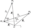Fig. 1 Three-body problem from an inertial frame and from a mi-relative frame.

2 The creep tide model for the 3BP

Let us consider the extended 3BP with masses m_i, m_j, and m_k and respective mean radii ${\mathcal{R}}_i$, ${\mathcal{R}}_j$, and ${\mathcal{R}}_k$. In addition, let us assume that the orbital motion of the bodies lies in the same plane and the spin vectors are perpendicular to it. From an arbitrary inertial frame, let R_i, R_j, and R_k be the respective position vectors of m_i, m_j, and m_k. We denote the relative position of m_j to m_i by Δ_ji = R_j −R_i, while the angle subtended between the position of m_j and the reference axis, as seen from m_i, is called φ_ji (the same for j = k, see Fig. 1).

Our goal is to study the spin dynamics of these three bodies under the effects of their mutual tidal perturbations. The tides will be modelled using the creep theory (Ferraz-Mello 2013, 2015a) in its closed form (Folonier et al. 2018) and extended to the case of three interacting masses.

2.1 Equilibrium figure

As a consequence of the gravitational interaction on extended bodies, each mass m_i undergoes a deformation which is given by the superposition of the tidal interaction with the two companions m_j and m_k. In this work, we also consider the rotational flattening on each body due to its own spin, and assume that the resulting deformation due to theseeffects is small enough that a model developed up to the first order of the flattenings (like the one we develop in this work) represents an accurate description of the problem.

If we consider that each mass m_i is a perfect fluid that instantly responds to any external stress, it will immediately adopt an equilibrium figure determined by the tides raised by the two companions (i.e. static tides) and its own rotation. The surface equation of this equilibrium figure seen from the centre of mass, is determined by giving the distance ρ_i of an arbitrary point on its surface with co-latitude angle θ_i and longitude angle φ_i. It can be expressed as the sum of the interactions between pairs as (Tisserand 1891; Folonier et al. 2015) $$\begin{array}{ll}{\rho }_i({\theta }_i,{\phi }_i)=\hfill & {\mathcal{R}}_i[1+({ϵ}_i^M+\frac{{ϵ}_{ij}^{\rho }}{2}+\frac{{ϵ}_{ik}^{\rho }}{2})(\frac{1}{3}-{\cos }^2{\theta }_i)\hfill \\ \hfill & +\frac{1}{2}{\sin }^2{\theta }_i({ϵ}_{ij}^{\rho }\cos (2{\phi }_i-2{\phi }_{ji})+{ϵ}_{ik}^{\rho }\cos (2{\phi }_i-2{\phi }_{ki}))]\hfill \end{array}$$(1)

where we have chosen the same definitions for the flattening as in Folonier et al. (2018), given by 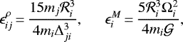$$\begin{array}{lll}{ϵ}_{ij}^{\rho }=\frac{15m_j{\mathcal{R}}_i^3}{4m_i{\Delta }_{ji}^3},\hfill & \hfill & {ϵ}_i^M=\frac{5{\mathcal{R}}_i^3{\Omega }_i^2}{4m_i\mathcal{G}},\hfill \end{array}$$(2)

with Ω_i being the spin module of m_i and $\mathcal{G}$ the gravitational constant.

We propose that the equilibrium figure expressed in Eq. (1) corresponds to an equivalent triaxial flat ellipsoid with equatorial flattening ${ϵ}_i^{\rho }$, polar flattening ${ϵ}_i^z$, and equilibrium orientation defined by the unit vector 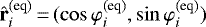${\widehat{r}}_i^{(\text{eq})}=(\cos {\phi }_i^{(\text{eq})},\sin {\phi }_i^{(\text{eq})})$ (see left panel of Fig. 2). The surface equation of this equivalent equilibrium figure is simply given by $$\begin{array}{ll}{\rho }_i({\theta }_i,{\phi }_i)\hfill & ={\mathcal{R}}_i[1+{ϵ}_i^z(\frac{1}{3}-{\cos }^2{\theta }_i)+\frac{{ϵ}_i^{\rho }}{2}{\sin }^2{\theta }_i\cos (2{\phi }_i-2{\phi }_i^{\text{eq}}).]\hfill \end{array}$$(3)

The equivalent flattenings and orientation can be obtained in terms of the two-body interacting parameters by equating Eqs. (3) and (1). This results in 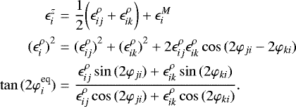$$\begin{array}{lll}{ϵ}_i^z\hfill & =\hfill & \frac{1}{2}({ϵ}_{ij}^{\rho }+{ϵ}_{ik}^{\rho })+{ϵ}_i^M\hfill \\ {({ϵ}_i^{\rho })}^2\hfill & =\hfill & {({ϵ}_{ij}^{\rho })}^2+{({ϵ}_{ik}^{\rho })}^2+2{ϵ}_{ij}^{\rho }{ϵ}_{ik}^{\rho }\cos (2{\phi }_{ji}-2{\phi }_{ki})\hfill \\ \tan (2{\phi }_i^{\text{eq}})\hfill & =\hfill & \frac{{ϵ}_{ij}^{\rho }\sin (2{\phi }_{ji})+{ϵ}_{ik}^{\rho }\sin (2{\phi }_{ki})}{{ϵ}_{ij}^{\rho }\cos (2{\phi }_{ji})+{ϵ}_{ik}^{\rho }\cos (2{\phi }_{ki})}.\hfill \end{array}$$(4)

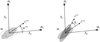Fig. 2 Left: equilibrium figure in the 3BP. Dashed-empty ellipsoids correspond to the static tidal deformations generated by each of the perturbing masses, while the resulting equilibrium figure of mi (Eq. (3)) is shown by a filled grey ellipsoid. The unit vector ${\widehat{r}}_i^{(\text{eq})}$ indicates the orientation of the equivalent equilibrium bulge. Right: real figure in the 3BP. The dark grey filled ellipsoid represents the modelled real figure induced on mi when we take into account the internal viscosity; we note that it is displaced by an angle δi, with respectto the equilibrium figure and also has different flattenings.

2.2 Creep equations

Now, we assume the more realistic case in which each body has a certain viscosity that does not allow it to attain the equilibrium figure instantly. The real shape of m_i, measured by the surface distance ζ_i(θ_i, φ_i), is also modelled as a triaxial flat ellipsoid but is characterised by the equatorial flattening ${\mathcal{E}}_i^{\rho }$ and polar flattening ${\mathcal{E}}_i^z$. On the other hand, the orientation of the real figure is displaced with respect to the equilibrium orientation by a lag δ_i. Therefore, the real orientation unit vector is ${\widehat{r}}_i^{(b)}=(\cos ({\phi }_i^{(\text{eq})}+{\delta }_i),\sin ({\phi }_i^{(\text{eq})}+{\delta }_i))$ (see right panel in Fig. 2). Thus, the surface equation of the real flat ellipsoid is then given by $$\begin{array}{lll}{\zeta }_i({\theta }_i,{\phi }_i)\hfill & =\hfill & {\mathcal{R}}_i[1+{\mathcal{E}}_i^z(\frac{1}{3}-{\cos }^2{\theta }_i)\hfill \\ \hfill & \hfill & +\frac{{\mathcal{E}}_i^{\rho }}{2}{\sin }^2{\theta }_i\cos (2{\phi }_i-2({\phi }_i^{eq}+{\delta }_i))].\hfill \end{array}$$(5)

Contrary to Darwin-based tidal models, in the creep tide theory we assume that $({\mathcal{E}}_i^{\rho },{\mathcal{E}}_i^z,{\delta }_i)$ are a priori unknown quantities whose values at each instant of time are obtained by solving the creep equation: $${\dot{\zeta }}_i+{\gamma }_i{\zeta }_i={\gamma }_i{\rho }_i,$$(6)

where γ_i is the so-called relaxation factor of m_i (Ferraz-Mello 2013) which is inversely proportional to the body viscosity and is assumed to be constant in this work.

A set of three differential equations for the shape and orientation of the real figure of m_i can be obtained by differentiating Eq. (5) with respect to time, introducing its expression plus Eqs. (3) and (5) into Eq. (6) and identifying terms of equal dependence with (θ_i, φ_i) (see Folonier et al. 2018). Particularly, it is convenient to express the equatorial flattening and orientation in terms of regular variables as in Gomes et al. (2019) as $$\begin{array}{lll}\stackrel{.}{X_i}\hfill & =\hfill & -{\gamma }_i{X}_i-2Y_i({\Omega }_i-{\stackrel{.}{{\phi }_i}}^{\text{eq}})+{\gamma }_i{ϵ}_i^{\rho }\hfill \\ \stackrel{.}{Y_i}\hfill & =\hfill & -{\gamma }_i{Y}_i+2X_i({\Omega }_i-{\stackrel{.}{{\phi }_i}}^{\text{eq}})\hfill \\ \stackrel{.}{{\mathcal{E}}_i^z}\hfill & =\hfill & {\gamma }_i({ϵ}_i{}^z-{\mathcal{E}}_i{}^z)\hfill \end{array}$$(7)

where the regular variables are defined as $$\begin{array}{lll}{X}_i={\mathcal{E}}_i^{\rho }\cos (2{\delta }_i);\hfill & \hfill & Y_i={\mathcal{E}}_i^{\rho }\sin (2{\delta }_i).\hfill \end{array}$$(8)

By comparing Eq. (7) with the shape and orientation evolution equations in the 2BP (e.g. Folonier et al. 2018; Gomes et al. 2019), we note that in the 3BP the creep equations maintain the same form, which makes the formalism applicable to any N-body problem. Thus, the complexity in the multi-body problem is only reduced to calculate the equilibrium figures.

2.3 Tidal forces and torques

At any instant of time, given the rotation frequency Ω_i of the body m_i, it is possible to calculate its real shape and orientation by solving the differential equation system (7). With these quantities, it is then possible to calculate the tidal forces and torques between each pair of bodies.

The tidal potential induced on m_j due to the deformation of m_i can be calculated as (e.g. Murray & Dermott 1999) $$\begin{array}{ll}{U}_{ji}({\Delta }_{ji})\hfill & =-\frac{G(B_i-A_i)}{2{\Delta }_{ji}^3}(3{({\widehat{\Delta }}_{ji}\cdot {\widehat{r}}_i^b)}^2-1)-\frac{G(C_i-B_i)}{2{\Delta }_{ji}^3},\hfill \end{array}$$(9)

where A_i, B_i, C_i are the principal moments of inertia of m_i, which can be related to the ellipsoidal flattenings (see Appendix A of Folonier et al. 2015) as: 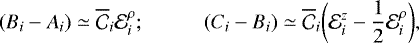$$(B_i-A_i)\simeq {\overline{\mathcal{C}}}_i{\mathcal{E}}_i^{\rho };(C_i-B_i)\simeq {\overline{\mathcal{C}}}_i({\mathcal{E}}_i^z-\frac{1}{2}{\mathcal{E}}_i^{\rho }),$$(10)

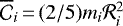where ${\overline{\mathcal{C}}}_i=(2/5)m_i{\mathcal{R}}_i^2$ is the principal moment of inertia of a homogeneous spherical body of mass m_i and radius ${\mathcal{R}}_i$.

The tidal force applied on m_j due to the deformation of m_i can be simply calculated as: $$\begin{array}{lll}{F}_{ji}\hfill & =\hfill & -m_j{\nabla }_{{\Delta }_{ji}}{U}_{ji}\hfill \\ \hfill & =\hfill & \frac{3G{m}_j{\overline{\mathcal{C}}}_i}{2{\Delta }_{ji}^5}{\mathcal{E}}_i^{\rho }\sin (2({\phi }_i^{\text{eq}}+{\delta }_i)-2{\phi }_{ji})(\widehat{k}\times {\Delta }_{ji})\hfill \\ \hfill & \hfill & -\frac{3G{m}_j{\overline{\mathcal{C}}}_i}{2{\Delta }_{ji}^5}(\frac{3}{2}{\mathcal{E}}_i^{\rho }\cos (2({\phi }_i^{\text{eq}}+{\delta }_i)-2{\phi }_{ji})+{\mathcal{E}}_i^z){\Delta }_{ji},\hfill \end{array}$$(11)

where we have decomposed ${\widehat{r}}_i^b$ in terms of the radial unit vector ${\widehat{\Delta }}_{ji}$ and the azimutal unit vector ($\widehat{k}\times$ ${\widehat{\Delta }}_{ji}$) ($\widehat{k}$ is the unit vector paralell to the spin vectors).

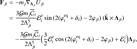
The torque induced on m_j due to the deformation of m_i can be simply calculated as $$\begin{array}{ll}{T}_{ji}\hfill & ={\Delta }_{ji}\times F_{ji}\hfill \\ \hfill & =\frac{3G{m}_j{\overline{\mathcal{C}}}_i}{2{\Delta }_{ji}^3}{\mathcal{E}}_i^{\rho }\sin (2({\phi }_i^{\text{eq}}+{\delta }_i)-2{\phi }_{ji})\widehat{k},\hfill \end{array}$$(12)

while a completely analogous expression can be found for the torque applied on m_k due to the deformation of m_i by exchanging the indexes.

Now, we assume that the reaction torque due to the deformation on m_i is the only responsible for changing its own rotational velocity. This is a natural assumption that satisfies the condition that the variation of the rotation speed of m_i should be cancelled in the limit ${\mathcal{R}}_i\to 0$ (Zoppetti et al. 2019). Thus, the rotational evolution of m_i is given by $$\begin{array}{lll}{C}_i{\stackrel{.}{\Omega }}_i+{\dot{C}}_i{\Omega }_i\hfill & =\hfill & -(T_{ji}+T_{ki})\hfill \\ \hfill & =\hfill & -\frac{3G{\overline{\mathcal{C}}}_i{\mathcal{E}}_i^{\rho }}{2}[\frac{m_j}{{\Delta }_{ji}^3}\sin (2({\phi }_i^{\text{eq}}+{\delta }_i)-2{\phi }_{ji})\hfill \\ \hfill & \hfill & +\frac{m_k}{{\Delta }_{ki}^3}\sin (2({\phi }_i^{\text{eq}}+{\delta }_i)-2{\phi }_{ki})]\widehat{k}\hfill \end{array}$$(13)

Neglecting the term corresponding to the variation of the polar moment of inertia (i.e. Ċ_i ~ 0), using Eq. (4) and after some algebra, it is possibly to find that the rotational evolution of the body m_i is governed by $${\dot{\Omega }}_i=-\frac{2G{m}_i}{5{\mathcal{R}}_i^3}{ϵ}_i^{(\rho )}{Y}_i$$(14)

The set of differential equations formed by Eqs. (7) and (14) describe the dynamical evolution of the system on short timescales and investigating this latter process is the target of this work.

3 Numerical simulations

Circumbinary planetary systems are particularly interesting scenarios where we can study the effects of tides on dynamical evolution in the framework of the 3BP. In this context, the stellar tidal evolution is expected to be only very weakly affected by the presence of the CB planet and mainly dominated by the two-body interaction between the binary components (Correia et al. 2016; Zoppetti et al. 2019). As the rotational evolution due to tides in a binary system has been extensively studied (e.g. Mignard 1979; Hut 1981; Efroimsky 2012), in this paper we focus on the evolution of the planet.

Using a CTL model based on the tidal forces and torques of Mignard (1979), in Zoppetti et al. (2019, 2020) we found that the characteristic timescales of the rotational evolution of any planet in a Kepler-like circumbinary system are much shorter than the characteristic timescales of the orbital evolution of the system. As a result, in this framework, while the shape, orientation, and rotationof each body reach a stationary solution, only periodic oscillations are expected in the orbital elements of the bodies, except for the fast angles. For this reason, in this work we take advantage of this adiabatic nature of the problem and solve the set of differential equations associated with the evolution of the shape of each body, its orientation, and its rotation (Eqs. (7) and (14)), assuming fixed values for all the orbital elements except the true anomalies. The orbital evolution of the bodies on much longer timescales will be addressed in a forthcoming work.

With this motivation, we begin first by analysing the results of the numerical integrations of Eqs. (7) and (14) in a 3BP consisting of a single planet around a binary star. To compare with the results of our previous works (Zoppetti et al. 2018, 2019), we choose a Kepler-38-like system as a test case. Nominal values for system parameters and initial orbital elements are detailed in Table 1. Stellar masses and radii were taken close to those observed by Orosz et al. (2012a), while the value of m₂ was estimated from a semi-empirical mass–radius fit (Mills & Mazeh 2017).

The first obstacle we encountered when performing the numerical integration was the extreme difficulty in solving the equations system numerically for bodies with large relaxation factors (γ₂ ≫ n₁, n₂), typically associated with bodies with a large gaseous component (Ferraz-Mello 2013). This limitation comes from the fact that, for large γ-values, the shape and orientation of the deformed body quickly adapt to the change in position of the deforming bodies, so the integrator must greatly reduce the time-step to pursue their instantaneous positions and, finally, integration over timescales of millions of years becomes computationally impractical (e.g. Lambert 1991). However, as we see below, the rotational evolution timescales can be extrapolated from the simulations of more viscous bodies in the same regime and the synchronous attractor from the analytical solution calculated in Sect. 4.

In Fig. 3 we show the rotational evolution of a CB planet from a Jacobi reference frame, obtained by direct numerical integration of Eqs. (7) and (14). All initial conditions and system parameters were taken equal to the nominal values summarised in Table 1, while the angles were set equal to zero. As mentioned above, the orbital elements are considered fixed, with the exception of the mean anomalies which vary linearly with time.

Many interesting features can be noted in Fig. 3. We begin first by identifying, as in the 2BP, two different regimes whose boundary value is close to the main dynamical frequency of the problem n₂ : the ‘stiff regime’ for γ₂ < n₂ and the ‘gaseous regime’ for γ₂ > n₂. In the stiff regime, the rotational evolution acquires its stationary value faster the higher the relaxation factor γ₂, while the opposite occurs in the gaseous limit: if we decrease the planetary viscosity (increase γ₂) the attractor is reached on longer timescales. This bimodal character of the energy dissipation was observed previously in the 2BP (Ferraz-Mello 2013; Correia et al. 2014). For relaxation parameters far from the maximum, the energy dissipation decreases proportional to γ₂ in the gaseous regime and decreases inversely proportional to γ₂ in the stiff bodies limit.

In the stiff regime, we see from the upper left panel of Fig. 3 that for bodies with very small relaxation factors γ₂ ∕n₂ ~ 0.01, (i.e. γ₂ ≃ 7 × 10⁻⁹ Hz), the planetary spin captures may occur in an attractor different from 1:1 spin–orbit resonance; in our testing case 3:2 with an associated circularisation of the lag-angle δ₂. This result is expected from the 2BP experiment, where for very low γ₂ -values, the probability of capture in this type of resonance increases considerably (Correia et al. 2014; Gomes et al. 2019). However, according to our numerical simulations, captures in resonances different from the 1:1 seems to occur for bodies with satellite-like relaxation factors like the moon, which are expected to be approximately two orders of magnitude lower than those expected for rocky earth-type planets (Ferraz-Mello 2013), or for bodies with high initial eccentricities, a case that we do not consider in this work. This particular stationary state also has a counterpart in the flattenings ${\mathcal{E}}_2^{\rho }$ and ${\mathcal{E}}_2^z$, which oscillate around values significantly different from those in the case of the capture in the 1:1 spin–orbit resonance (see lower panels in Fig. 3).

The oscillation of the lag-angle around δ₂ ~ 45° of free rotating bodies in the stiff regime can be observed in the upper right panel of Fig. 3 (blue and orange dots). This result was also previously reported in the framework of the 2BP (Gomes et al. 2019) and is mainly due to the lack of the elastic tide component inside the creep model (Ferraz-Mello 2015b). Finally, we notice that in this limit, the oscillations of δ₂ (and also of Ω₂, although it cannot be distinguished in the upper left panels) around the stationary values are of much greater amplitudes than those in the gaseous regime, while the completely opposite situation occurs for ${\mathcal{E}}_2^{\rho }$ and ${\mathcal{E}}_2^z$. As noticed by Folonier et al. (2018) in the 2BP, these periodic oscillations with large amplitudes must be taken into account when constructing an analytical approach (see Sect. 4).

Regarding the gaseous regime, despite considering bodies of different viscosity (i.e. relaxation factors γ₂), we observe similar behaviours: stationary spins are located very close to n₂ and the lag-angle δ₂ oscillates close to zero, with low oscillation amplitudes. If we omit the case of γ₂ ∕n₂ = 1 which is a behaviour change value, we can observe in the secondary plot of the upper left panel that the equilibrium spins become smaller as we increase γ₂ and turn out to be subsynchronous for this parameters system in the gaseous regime (see red and magenta curves). However, despite the fact that the rotational equilibrium state resulting from the numerical integrations appears to be subsynchronous in the gaseous limit, this solution is far from the one we found in Zoppetti et al. (2019) (dashed black line in the upper left panel). The details of the 1:1 spin–orbit mean solution are described in Sect. 4, while the reasons for the discrepancy with Zoppetti et al. (2019) are discussed in Sect. 5.

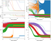Fig. 3 Rotational evolution due to tides in a Kepler-38-like CB planet (see Table 1), considering different values of planetary relaxation factor γ2, illustrated here with different colours (see legend in the upper left panel). The evolution was calculated by direct numerical integration of Eqs. (7) and (14). The evolution of the planetary spin rate Ω2 is shown in the upper left panel (zoomed around Ω2 ~ n2 in a secondary plot), the lag-angle δ2 in the upper right panel, the equatorial flattening ${\mathcal{E}}_2^{\rho }$ in the lower left panel and the polar flattening ${\mathcal{E}}_2^z$ in the lower right panel. The dashed black line in the upper left panel shows the stationary solution predicted by Zoppetti et al. (2019) with a CTL-based model.

4 An analytical solution for the mean rotational stationary state

As discussed in the previous Sect. 3, according to our numerical simulations, the rotational evolution due to tides of a CB planet in a low-eccentric orbit with γ₂ ≳ 0.1n₂ (approximately the expected range for a planet-like body, according to Ferraz-Mello 2013) tends to be captured in the 1:1 spin–orbit resonance.

The timescales for the capture depend on the planetary viscosities. While for bodies in the stiff regime are expected to be approximately of the order of millions of years, in the gaseous regime they can be of the order of billions of years, considering a γ₂ -value similar to the one estimated for Neptune (Ferraz-Mello 2013) and extrapolating the behaviour observed in Fig. 3 by assuminga linear dependence of the decay times with the relaxation factors. Although for giant planets these timescales may be even larger than the age of the systems, the enormous uncertainty that exists regarding the internal structure of the exoplanets, and in particular the CB Kepler planets, prohibits a reliable estimate of the planetary relaxation factor. In addition to this, the central binary could have undergone an important change in both the physical parameters and the orbital elements, which may have accelerated the tidal evolution processes (Zoppetti et al. 2018). In summary, according toour model, a CB planet in a Kepler-38-like system with a large rocky component is expected to have reached its stationary spin and this is also possible for the case of gaseous CB planets with small relaxation factors γ₂.

From a practical point of view, having an analytical approach for the rotational stationary state will allow us, when studying the long-term orbital evolution of the system, to avoid direct numerical integration of the Eqs. (7) and (14), which are particularly difficult to solve for bodies with large relaxation factors (see Sect. 3) and, instead, to work with a semi-analytical approach in which we introduce a recipe for the equilibrium shape, orientation, and spin.

With these motivations, in this section we develop an analytical approximation for the system of Eqs. (7) and (14) around the pseudo-synchronous stationary state, where in this particular scenario where there are two central bodies (both stellar components of the binary) exerting tides onto a planet. Mathematically speaking, our goal is to find the stationary solution for the system formed by $(X_2,Y_2,{\mathcal{E}}_2^z)$ and Ω₂, employing a power series truncated in α = a₁∕a₂, e₁, and e₂.

To do this, we first adopt a Jacobi reference frame for the coordinates and velocities of the bodies, where the state vector of m₁ is defined as m₀ -centric, while the state vector of m₂ is measured with respect to the barycentre of m₀ and m₁. We note that these coordinates and velocities are required to compute the forcing terms given by ${\stackrel{.}{{\phi }_i}}^{\text{eq}}$, ${ϵ}_i^{\rho }$, and ${ϵ}_i{}^z$ in our differential equation system.

Regarding the resolution method, we choose the same path as the one taken in Appendix 2 of Folonier et al. (2018), which consists in proposing a particular stationary solution, which takes inspiration from the form (i.e. dependence on fundamental frequencies) of the elliptical expansions of the forced terms ${ϵ}_i^{\rho }$ and ${\stackrel{.}{{\phi }_i}}^{\text{eq}}$. In this case, we propose a solution of the form $$\begin{array}{lll}{\Omega }_2\hfill & =\hfill & {\sum }_{\mathcal{l}}{\left\{{\Omega }_2\right\}}_{\mathcal{l}}\cos (l_1{M}_1+l_2{M}_2+l_3{\varpi }_1+l_4{\varpi }_2-{\Phi }_{\mathcal{l},{\Omega }_2})\hfill \\ X_2\hfill & =\hfill & {\sum }_{\mathcal{l}}{\left\{X_2\right\}}_{\mathcal{l}}\cos (l_1{M}_1+l_2{M}_2+l_3{\varpi }_1+l_4{\varpi }_2-{\Phi }_{\mathcal{l},X_2})\hfill \\ Y_2\hfill & =\hfill & {\sum }_{\mathcal{l}}{\left\{Y_2\right\}}_{\mathcal{l}}\cos (l_1{M}_1+l_2{M}_2+l_3{\varpi }_1+l_4{\varpi }_2-{\Phi }_{\mathcal{l},Y_2})\hfill \\ {\mathcal{E}}_2^z\hfill & =\hfill & {\sum }_{\mathcal{l}}{\left\{{\mathcal{E}}_2^z\right\}}_{\mathcal{l}}\cos (l_1{M}_1+l_2{M}_2+l_3{\varpi }_1+l_4{\varpi }_2-{\Phi }_{\mathcal{l},{\mathcal{E}}_2^z}),\hfill \end{array}$$(15)

where M₁ and ϖ₁ are the mean anomaly and pericentre longitude of the secondary star, while M₂ and ϖ₂ are those corresponding to the planet. The amplitudes ${\left\{w\right\}}_{\mathcal{l}}$ and the constant phases Φ_ℓ,x depend on the subscripts ℓ = (l₁, l₂, l₃, l₄) and each variable w = Ω₂, X₂, Y₂ or ${\mathcal{E}}_2^z$. This particular solution and its derivatives are then introduced into the systems (7) and (14), and the coefficients can be calculated by equating the terms with the same trigonometric argument and neglecting terms of higher-order. The terms in system (15) with l₁ = l₂ = 0 correspond to the mean stationary solution and are given in what follows. We choose to express the stationary solution of the rotational evolution written in terms of the mean planetary spin ⟨Ω₂ ⟩, mean planetary lag-angle ⟨δ₂ ⟩, mean planetary equatorial flattening $\langle {\mathcal{E}}_2^{\rho }\rangle$, and mean planetary polar flattening $\langle {\mathcal{E}}_2^z\rangle$. Up to third order in α = a₁∕a₂ and to second order in the eccentricities e₁ and e₂, including also the contribution of the fourth-order and sixth-order terms that do not depend on the eccentricities, the solution is explicitly given by $$\begin{array}{lll}\langle {\Omega }_2\rangle \hfill & =\hfill & n_2+6\frac{{\gamma }_2^2{n}_2}{{\gamma }_2^2+n_2^2}{e}_2^2+5\frac{{\gamma }_2^2{n}_2}{{\gamma }_2^2+n_2^2}{e}_2^2{\mathcal{M}}_2{\alpha }^2\hfill \\ \hfill & \hfill & -\frac{325}{16}\frac{{\gamma }_2^2{n}_2}{{\gamma }_2^2+n_2^2}{e}_1{e}_2\cos (\Delta \varpi ){\mathcal{M}}_3{\alpha }^3\hfill \\ \hfill & \hfill & -\frac{19}{2}\frac{{\gamma }_2^2(2n_1-2n_2)}{{\gamma }_2^2+{(2n_1-2n_2)}^2}{\mathcal{M}}_2^2{\alpha }^4+{\langle {\Omega }_2\rangle }_{o6}.\hfill \end{array}$$(16) $$\begin{array}{lll}\langle {\delta }_2\rangle \hfill & =\hfill & 6\frac{{\gamma }_2{n}_2}{{\gamma }_2^2+n_2^2}{e}_2^2+5\frac{{\gamma }_2{n}_2}{{\gamma }_2^2+n_2^2}{e}_2^2{\mathcal{M}}_2{\alpha }^2\hfill \\ \hfill & \hfill & -[\frac{325}{16}{\gamma }_2\cos (\Delta \varpi )+\frac{175}{32}{n}_2\sin (\Delta \varpi )]\frac{n_2}{{\gamma }_2^2+n_2^2}{e}_1{e}_2{\mathcal{M}}_3{\alpha }^3\hfill \\ \hfill & \hfill & -\frac{19}{2}\frac{{\gamma }_2(2n_1-2n_2)}{{\gamma }_2^2+{(2n_1-2n_2)}^2}{\mathcal{M}}_2^2{\alpha }^4+{\langle {\delta }_2\rangle }_{o6}\hfill \end{array}$$(17) $$\begin{array}{lll}\frac{\langle {\mathcal{E}}_2^{\rho }\rangle }{{\overline{ϵ}}_2^{\rho }}\hfill & =\hfill & 1+(\frac{3}{2}-4\frac{n_2^2}{{\gamma }_2^2+n_2^2})e_2^2\hfill \\ \hfill & \hfill & +[\frac{5}{4}+\frac{15}{8}{e}_1^2+(\frac{25}{4}-5\frac{n_2^2}{{\gamma }_2^2+n_2^2})e_2^2]{\mathcal{M}}_2{\alpha }^2\hfill \\ \hfill & \hfill & -\frac{25}{8}\frac{(3n_2^2+5{\gamma }_2^2)}{{\gamma }_2^2+n_2^2}{e}_1{e}_2\cos (\Delta \varpi ){\mathcal{M}}_3{\alpha }^3\hfill \\ \hfill & \hfill & +[\frac{105}{64}{\mathcal{M}}_4+\frac{4{\gamma }_2^2{\mathcal{M}}_2^2}{{\gamma }_2^2+{(2n_1-2n_2)}^2}]{\alpha }^4+\frac{{\langle {\mathcal{E}}_2^{\rho }\rangle }_{o6}}{{\overline{ϵ}}_2^{\rho }}\hfill \end{array}$$(18) $$\begin{array}{lll}\frac{\langle {\mathcal{E}}_2^z\rangle }{{\overline{ϵ}}_2^M}\hfill & =\hfill & (1+12\frac{{\gamma }_2^2}{{\gamma }_2^2+n_2^2}{e}_2^2+10\frac{{\gamma }_2^2}{{\gamma }_2^2+n_2^2}{e}_2^2{\mathcal{M}}_2{\alpha }^2\hfill \\ \hfill & \hfill & -\frac{325}{8}\frac{{\gamma }_2^2}{{\gamma }_2^2+n_2^2}{e}_1{e}_2\cos (\Delta \varpi ){\mathcal{M}}_3{\alpha }^3\hfill \\ \hfill & \hfill & -19\frac{(2n_1-2n_2){\gamma }_2^2}{n_2({\gamma }_2^2+{(2n_1-2n_2)}^2)}{\mathcal{M}}_2^2{\alpha }^4)\hfill \\ \hfill & \hfill & +\frac{{\overline{ϵ}}_2^{\rho }}{{\overline{ϵ}}_2^M}(\frac{1}{2}+\frac{3}{4}{e}_2^2+[\frac{9}{8}+\frac{27}{16}{e}_1^2+\frac{45}{8}{e}_2^2]{\mathcal{M}}_2{\alpha }^2\hfill \\ \hfill & \hfill & -\frac{225}{16}{e}_1{e}_2\cos (\Delta \varpi ){\mathcal{M}}_3{\alpha }^3+\frac{225}{128}{\mathcal{M}}_4{\alpha }^4)+\frac{{\langle {\mathcal{E}}_2^z\rangle }_{o6}}{{\overline{ϵ}}_2^M}\hfill \end{array}$$(19)

where ${\langle {\Omega }_2\rangle }_{o6}$, ${\langle {\delta }_2\rangle }_{o6}$, ${\langle {\mathcal{E}}_2^{\rho }\rangle }_{o6}$ and ${\langle {\mathcal{E}}_2^z\rangle }_{o6}$ are the terms independent of the eccentricities, expanded up to sixth order in α and listed in the appendix. We mention that the fifth-order terms are dependent on eccentricities and were therefore excluded from this approximation. The mass factors are defined in terms of the binary mass ratio β = m₁∕m₀ as $${\mathcal{M}}_2=\frac{\beta }{{(1+\beta )}^2},{\mathcal{M}}_3=\frac{\beta -{\beta }^2}{{(1+\beta )}^3},{\mathcal{M}}_4=\frac{\beta -{\beta }^2+{\beta }^3}{{(1+\beta )}^4},$$(20)

and the equilibrium mean flattenings are given by $$\begin{array}{lll}{\overline{ϵ}}_2^{\rho }=\frac{15(m_0+m_1){\mathcal{R}}_2^3}{4m_2{a}_2^3}\hfill & \text{and}\hfill & {\overline{ϵ}}_2^M=\frac{5{\mathcal{R}}_2^3{n}_2^2}{4m_2\mathcal{G}}.\hfill \end{array}$$(21)

We first note from expressions (16)–(19) that the mean solutions depend on the mean orbital configuration mainly through e₂ up to low orders in α, but also through e₁ and Δϖ up to higher orders. The dependence of the expressions on the masses m₀ and m₁, and the semimajor axis ratio α are given in such a way that when m₁ → 0 (i.e. a secondary star of very low mass) or α → 0 (i.e. a planet far away from the binary), and we recover the 2BP expressions of Folonier et al. (2018).

On the other hand, according to preliminary numerical simulations, the mean rotational solutions only exhibit a very weak dependence with e₁. This fact is also expected if we notice that, in the mean analytical expression, the functional dependence with this parameter only appears up to third order in α.

Another interesting feature of the mean solutions is the strong correlation between the stationary spin ⟨Ω₂ ⟩ with the lag angle ⟨δ₂ ⟩: if we neglect the dependence on Δϖ (e.g. for aligned and non-evolving pericentres or for the circulating case), these quantities are simply related as ⟨Ω₂ ⟩− n₂ = ⟨δ₂⟩∕γ₂. As a result, a sub- or supersynchronous mean stationary rotation speed is directly associated with a delay or advance of the tidal bulge, respectively.

The rheology of the planet is taken into account through the ratio mainly between the relaxation factor γ₂ and the main frequency of the problem n₂. However, up to higher α-order, other frequencies such as 2n₁ − 2n₂ start become important in the solutions. For this reason, as we mention in Sect. 3, the exact position of the frontier between the stiff regime and the gaseous regime is expected to be close to γ₂ = n₂, but not exactly at this point.

In Fig. 4, we compare the mean values of ⟨Ω₂ ⟩, ⟨δ₂ ⟩, $\langle {\mathcal{E}}_2^{\rho }\rangle$, and $\langle {\mathcal{E}}_2^z\rangle$ obtained with different methods, as a function of the normalised relaxation factor γ₂ ∕n₂. The full-line curves indicate the results of a numerical integration from an initial condition far from the equilibrium which is allowed to evolve towards the stationary state and is then filtered over the fast angles. The dashed-line curves represent the results obtained respectively with Eqs. (16)–(19), while the dotted-line curves represent the simplified 2BP case in which the central binary is replaced by a unique body with mass equal to the sum of the binary components. Large coloured dots represent the final mean value obtained with different γ₂ -values in simulations of Sect. 3, which result in a capture in the 1:1 spin–orbit resonance (see Fig. 3): the cases of γ₂ ∕n₂ = 0.1 (in orange), γ₂ ∕n₂ = 1 (in green), γ₂ ∕n₂ = 10 (in red) and γ₂∕n₂ = 100 (in magenta). We note that, in this last case, the magenta dots are not perfectly located on the blue full-line curves because this final condition, taken from the simulation of Fig. 3, is almost but still not perfectly in the stationary state.

Figure 4 allows us to observe the existence of the two different regimes mentioned in Sect. 3: the stiff regime for γ₂ < n₂ and the gaseous regime for γ₂ > n₂, where far enough away from the transition value ~n₂, the rotational equilibrium solution becomes independent of the planetary relaxation factor γ₂. In particular, in the case of the mean stationary speed ⟨Ω₂⟩ (upper left panel), planets in the stiff regime are expected to asymptotically synchronise their spins with the mean motion, independently of their orbital parameters, body masses and viscosities. This prediction is completely analogous to that expected with the 2BP (Folonier et al. 2018). However, a much greater variety of behaviours is seen in the gaseous regime: the stationary solutions do depend on the orbital parameters and binary component masses. In this regime, unlike what is expected in the 2BP (dotted curves), the presence of an inner secondary star leads to lower stationary spins, which can be subsynchronous, in the low planetary eccentric limit.

With respect to the accuracy of our analytical model in fitting the filtered numerical integrations, we observe that not only is it able to predict the subsynchronous solution of the spins, but it also gives a very precise estimation of the equilibrium solution in the complete range of γ₂ values. On the other hand, the 2BP simplification can also give a good prediction, but the accuracy of the approximation is strongly dependent on the initial condition and the relaxation factor range.

In Fig. 5, we evaluate with more detail the accuracy of our mean stationary solution given by expressions (16)–(19) as a function of the small parameters α = a₁∕a₂ and e₂ for the gaseous case γ₂ = 100n₂. Different α values were obtained by varying the semi-major axis of the planet a₂. Although it is not a small parameter of our model, we also explore a different secondary mass m₁.

We observe from Fig. 5 that our sixth-order analytical fit is a very precise estimation of the filtered numerical integrations for the rotational evolution of a CB planet in a Kepler-38-like system. This occurs even for high α values such as α ~ 0.4, where the planet is probably inside the instability limit imposed by the presence of an internal secondary disturber (e.g. Holman & Wiegert 1999). A good approximation is also obtained with the fourth-order fit. However, because most Kepler CB planets are located very close to binary (typically α ~ 0.3), a higher order approach is required to model its mean rotational behavior more accurately.

As expected, for the standard case (m₁ = 1∕4 m_⊙, right column) the 2BP simplification is only a good fit of the numerical simulation for low α values, where the tidal effects are probably of little importance. Curiously, the case of the mean polar flattening $\langle {\mathcal{E}}_2^z\rangle$ presents an exception: the numerical stationary solutions show little dependence on α and, while the sixth-order fit is the best fit in the complete range, the 2BP simplification is also a good approximation, even better than the fourth-order fit for planetary positions very close to the binary. This may seem less strange if we remember the expression of the equilibrium polar flattening ${ϵ}_i^z$ given in Eq. (4). Because of the definition of the flattenings chosen in this study (see Folonier et al. 2018), ${ϵ}_2^z$ contains terms that depend on the equatorial flattenings ${ϵ}_{2,0}^{\rho }$ and ${ϵ}_{2,1}^{\rho }$ which increase for higher α values, in addition to the classical Maclaurin flattening ${ϵ}_2^M$ which decreases as we move closer to the binary, because the stationary planetary spin also decreases. Thus, we expect a similar behaviour in the real polar flattening ${\mathcal{E}}_2^z$ that, because of a potential balance of these two contributions, may result in a weak dependence with α.

The case of m₁ = 1∕16 m_⊙ (left panels of Fig. 5) is considered as an illustrative example that exhibits the strong dependence of the solution with the secondary mass: for a low-mass secondary companion, the 2BP simplification begins to be a good approximation, especially for CB planets in wide orbits.

As an application example of our model predictions, in Fig. 6 we show a stationary spin map constructed with Eq. (16) for a CB planet in the gaseous regime γ₂ ∕n₂ = 100 located at α = 1∕3, as a function of its eccentricity e₂ and the binary mass ratio m₁ ∕m₀. The white curve represents the perfect synchronous state ⟨Ω₂⟩ = n₂, which divides the map into two regions: one where the stationary spins are expected to be supersynchronous (above), and another where subsynchronous spins are predicted (behind). With this reference, we can observe that the size of the subsynchronous region is proportionalto the normalised secondary mass, and tends to disappear for low mass secondary companion. In competition with m₁ ∕m₀, as we noticed in Zoppetti et al. (2019, 2020) and similar to that expected with the 2BP, the planetary eccentricity e₂ leads to more rapid stationary spins.

We have included in Fig. 6 the nominal location in the diagram of the Kepler CB planets observed very close to the binary and with an estimated mass which allows us to infer that they have an important gaseous component (m₂ ≳ m_Neptune): Kepler-16 (Doyle et al. 2011), Kepler-35 (Welsh et al. 2012), Kepler-38 (Orosz et al. 2012a), Kepler-47b (Orosz et al. 2012b), Kepler-64 (Schwamb et al. 2013), Kepler-413 (Kostov et al. 2014), and Kepler-1661 (Socia et al. 2020). If we assume that all these CB planets have an associated relaxation factor that satisfies γ₂ ≫ n₂ and that, in turn, these viscosities allowed them to have already reached their equilibrium state, then the expected stationary spins for them are typically subsynchronous. The exceptional case is Kepler-413, an eccentric CB planet orbiting a binary with two comparable-mass central stars, while Kepler-64 is expected to be very close to the perfect synchronous state. However, as we mention in Sect. 3, the amount of subsynchronous shift is much less important than the expected amount with the CTL tide model built in our previous works Zoppetti et al. (2019, 2020). The reasons for this difference are explained in detail in the following section.

Fig. 4 Mean rotational speed ⟨Ω2⟩ (upper left panel), mean lag-angle ⟨δ2⟩ (upper right panel), mean equatorial flattening $\langle {\mathcal{E}}_2^{\rho }\rangle$ (lower left panel) and mean polar flattening $\langle {\mathcal{E}}_2^z\rangle$ (lower right panel) as a function of the planetary relaxation factor normalised by the mean motion frequency γ2 ∕n2. The initial conditions for the system were taken from Table 1, but considering different planetary eccentricities, which are shown with curves of different colours as indicated in the upper left panel. Different types of curves represent different methods for obtaining the mean values: full-line curves represent the numerical results, dashed-line curves represent our sixth-order fit, and dotted-line curves represent the results of considering the 2BP with a central mass equal to the sum of the binary components. The vertical grey line in the upper left panel represents the position in the diagram of a solid Earth (Ferraz-Mello 2013) and the large coloured dots represent the final mean value obtained with different γ2 values, from simulations of Fig. 3 captured in the 1:1 spin–orbit resonance: γ2 ∕n2 = 0.1 (orange), γ2∕n2 = 1 (green), γ2∕n2 = 10 (red) and γ2∕n2 = 100 (magenta).

5 Revisiting the rotation of a CB planet in the CTL model

In the limit of gaseous bodies (i.e. γ₂ ≫ n₁, n₂), the stationary spin Eq. (16) expanded up to second order in α becomes $$\begin{array}{lll}{\langle {\Omega }_2\rangle }_{st}^{\text{gas}}\hfill & =\hfill & n_2+6n_2{e}_2^2+5n_2{e}_2^2{\mathcal{M}}_2{\alpha }^2.\hfill \end{array}$$(22)

We notice that this expression is different from the one we obtained in Eq. (22) of Zoppetti et al. (2019), using the classic CTL tidal model, based on the expressions of the direct torques of Mignard (1979). This section is dedicated to investigating the origin of this discrepancy and comparing these two different tidal models (i.e. CTL and creep) in the framework of the 3BP and thus to obtaining conclusions about the advantages and disadvantages of each one, in different contexts.

In Sect. 2.1 of Zoppetti et al. (2019) we used a simplified model to test the role of the cross tides in the 3BP with the CTL tidal model of Mignard (1979). We considered only one extended mass m₀ under tidal interaction of only one companion m₁ and used a third mass m₂ only as a test particle to evaluate the secular contribution of the cross torque whilst neglecting the gravitational perturbations of m₁. We used the usual astrocentric coordinate system centred on the extended mass. In that simplified system we found, employing numerical integrations and also analytical calculations, that the secular net contribution of the cross torques on the test particle were null. We then extrapolated that result to the general three-extended-body problem in a Jacobian frame and neglected the cross forces and tides of Mignard expressions. In what follows, we reformulate and improve the CTL model developed in Zoppetti et al. (2019) with the inclusion of the cross tides, and compare with our previous results.

Once again, we consider the 3BP composed of m_i, m_j, and m_k represented in Fig. 7, where between each pair of bodies we compute the complete tidal interaction, in addition to the gravitational forces. As a result of this consideration of the tides, due to the presence of each body m_i, one ellipsoid is generated on m_j and one ellipsoid on m_k. These figures are represented as grey ellipsoids on each respective mass of Fig. 7.

Let us use $F_{i,j}^k$ to denote the tidal force applied on m_i that is due to the ellipsoid that the presence of m_k generated on m_j. In Fig. 7, $F_{i,j}^k$ corresponds to the force applied on m_i due to the blue ellipsoid generated on m_j. Thus, if wetake into account all the action forces applied on m_i, we must consider the tides caused by the two ellipsoids that m_i itself generates on its companions (grey ellipsoids) plus the tides due to the cross ellipsoids (blue ellipsoid on m_j and red ellipsoid on m_k). On the other hand, to complete the force diagram, we also need to consider the reaction forces that m_i exerts on its two companions due to the ellipsoids generated on itself (blue and red ellipsoids on m_i). As a result, the total tidal force applied on m_i is given by 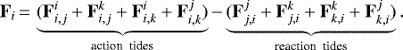$$F_i=\underset{\text{action}\text{tides}}{\underbrace{(F_{i,j}^i+F_{i,j}^k+F_{i,k}^i+F_{i,k}^j)}}-\underset{\text{reaction}\text{tides}}{\underbrace{(F_{j,i}^j+F_{j,i}^k+F_{k,i}^k+F_{k,i}^j)}}.$$(23)

We note that the forces with three different indexes in Eq. (23) correspond to the cross tides, which were neglected in Zoppetti et al. (2019), while the forces with two repeated indexes correspond to the direct tides, which we did consider in our previous work.

If we adopt the classical formalism of Mignard (1979) to model the tidal interactions between each pair of bodies, the explicit expression of the force $F_{i,j}^i$ is expanded up to first order in the time lag Δt_j as $$F_{i,j}^i=F_{i,j}^{k,(0)}+\Delta t_j{F}_{i,j}^{k,(1)},$$(24)

where (see Zoppetti et al. 2019) $$\begin{array}{lll}{F}_{i,j}^{k,(0)}\hfill & =\hfill & \frac{3}{2}\mathcal{G}{\mathcal{R}}_j^5{k}_{2,j}\frac{m_i}{{\Delta }_{ij}^5}\frac{m_k}{{\Delta }_{kj}^5}[2({\Delta }_{ij}\cdot {\Delta }_{kj}){\Delta }_{kj}\hfill \\ \hfill & \hfill & +({\Delta }_{kj}^2-\frac{5}{{\Delta }_{ij}^2}{({\Delta }_{ij}\cdot {\Delta }_{kj})}^2){\Delta }_{ij}],\hfill \end{array}$$(25) $$\begin{array}{lll}\hfill & \hfill & F_{i,j}^{k,(1)}=3\mathcal{G}{\mathcal{R}}_j^5{k}_{2,j}\frac{m_i}{{\Delta }_{ij}^5}\frac{m_k}{{\Delta }_{kj}^5}[\frac{({\Delta }_{kj}\cdot \stackrel{.}{{\Delta }_{kj}})}{{\Delta }_{kj}^2}(5{\Delta }_{kj}({\Delta }_{ij}\cdot {\Delta }_{kj})-{\Delta }_{kj}^2{\Delta }_{ij})\hfill \\ \hfill & \hfill & -[{\Delta }_{kj}\cdot ({\Omega }_j\times {\Delta }_{ij})+{\Delta }_{ij}\cdot \stackrel{.}{{\Delta }_{kj}}]{\Delta }_{kj}-[{\Delta }_{kj}\times {\Omega }_j+\stackrel{.}{{\Delta }_{kj}}]({\Delta }_{ij}\cdot {\Delta }_{kj})\hfill \\ \hfill & \hfill & +\frac{5}{{\Delta }_{ij}^2}{\Delta }_{ij}(({\Delta }_{ij}\cdot {\Delta }_{kj})[{\Delta }_{kj}\cdot ({\Omega }_j\times {\Delta }_{ij})+{\Delta }_{ij}\cdot \stackrel{.}{{\Delta }_{kj}}]\hfill \\ \hfill & \hfill & -\frac{({\Delta }_{kj}\cdot \stackrel{.}{{\Delta }_{kj}})}{2{\Delta }_{kj}^2}(5{({\Delta }_{ij}\cdot {\Delta }_{kj})}^2-{\Delta }_{ij}^2{\Delta }_{kj}^2))],\hfill \end{array}$$(26)

where k_2,j is the second-degree Love number of m_j.

The conservation of the total angular momentum of the system imposes that the total orbital angular momentum L_orb must satisfy $${\sum }_{i=0}^2{C}_i\stackrel{.}{{\Omega }_i}=-{\stackrel{.}{L}}_{\text{orb}},$$(27)

where the variation of the total orbital momentum can be written in terms of the relative positions as (Zoppetti et al. 2019) $$\begin{array}{lll}{\stackrel{.}{L}}_{\text{orb}}\hfill & =\hfill & {\Delta }_{j,i}\times (F_{j,i}^j+F_{j,i}^k)+{\Delta }_{k,i}\times (F_{k,i}^k+F_{k,i}^j)\hfill \\ \hfill & \hfill & +{\Delta }_{i,j}\times (F_{i,j}^i+F_{i,j}^k)+{\Delta }_{k,j}\times (F_{k,j}^k+F_{k,j}^i)\hfill \\ \hfill & \hfill & +{\Delta }_{i,k}\times (F_{i,k}^i+F_{i,k}^j)+{\Delta }_{j,k}\times (F_{j,k}^j+F_{j,k}^i).\hfill \end{array}$$(28)

As discussed in Sect. 4, Eq. (27) may be decoupled if we assume that the variation in the spin angular momentum of the body m_j is only due to the terms in the equation associated with its own deformation (see Zoppetti et al. 2019). Using this boundary condition, we have $$C_i{\stackrel{.}{\Omega }}_i=-[\underset{\text{direct}\text{torques}}{\underbrace{({\Delta }_{ji}\times F_{ji}^j+{\Delta }_{ki}\times F_{ki}^k)}}+\underset{\text{cross}\text{torques}}{\underbrace{({\Delta }_{ji}\times F_{ji}^k+{\Delta }_{ki}\times F_{ki}^j)}}]$$(29)

Again, we mention that the rotational evolution described by Eq. (15) of Zoppetti et al. (2019) only considers the direct torques, that is, the first two terms in Eq. (29).

In Fig. 8, we compare the different rotational evolution that results from the CTL tidal model of Mignard (1979) in the 3BP by considering the full expression in Eq. (29) and the version constructed neglecting the cross tides. The initial conditions were taken from Table 1, except for the initial planetary eccentricity which was varied: e₂ (0) = 0.05 in the upper panel and e₂(0) = 0.15 in the bottom panel. The full-line curves show the results of digitally filtered numerical integrations of Eq. (29), considering the full expression of the torque equation (in magenta) and neglecting the cross tides (in yellow). We have also included in these simulations the punctual gravitational interactions between the bodies in order to compare with our previous simulations of Zoppetti et al. (2019).

The comparison between the numerical integrations of the torque Eq. (29) without cross tides and the analytical results of the CTL model of Zoppetti et al. (2019) exhibited in Fig. 8 are analogous to the one presented inthe right panels of Fig. 7 of that work. However, here we adopt a tidal parameter $Q_{2^{\prime }}=3/(2n_2{k}_{2,2}\Delta t_2)$ that has been chosen in order that the associated relaxation factor satisfy γ₂ = 100n₂ (see Ferraz-Mello 2013) and, thus, the rotational evolution timescales be similar to the one presented in the magenta simulation of Fig. 3.

We first notice that the stationary solution of ⟨Ω₂⟩ exhibits long-term periodic oscillations, especially for the initially eccentric case. As mentioned in Zoppetti et al. (2019), this is due to the secular variation induced on the planetary eccentricity by the gravitational punctual interactions.

Regarding the comparison with the numerical simulations, we notice in both panels of Fig. 8 that the analytical model presented in Zoppetti et al. (2019) (brown curves) fits the stationary value of the planetary rotation very well when we neglect the cross tides in the torque equation. This is an expected result, because in the construction of that model, we took into account only the direct tidal forces and not the general expression of Eq. (26).

The comparison of the numerical integration for the full torque equation with the analytical results obtained with the creep model (in the gaseous limit) reveals two very important facts. On one hand, from the proximity of the magenta curves with the grey curves, we show that the results obtained for the rotational stationary state with the CTL tidal model of Mignard (1979) are the same as those obtained with the creep model in the limit of very large relaxation factor (γ₂ ≫ n₁, n₂). This result was checked in a completely analytical calculation by expanding the position and velocity vectors of Eq. (29) in α and the eccentricities, and then averaging with respect to both mean longitudes, with the help of an algebraic manipulator.

On the other hand, the difference between the magenta and yellow curves of Fig. 8 shows that, unlike what we assumed in Zoppetti et al. (2019) from analysing the simple case in which we considered only one extended mass and a reference frame in solidarity with it, the cross tides are not negligible in the general self-consistent problem of three extended masses. However, the physical effect that the tides – which are due to the presence of a binary (instead of a single star) – exert on an external planet is the same as what we reported in our previous works: it shifts the rotational stationary solution to lower spin values, by an amount that is proportional to the semimajor axis ratio α and the secondary mass m₁. The no-cross-tides model developed in Zoppetti et al. (2019, 2020) simply overestimates this effect.

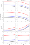Fig. 5 Mean rotational speed ⟨Ω2⟩ (first row panels), mean lag-angle ⟨δ2⟩ (second row panels), mean equatorial flattening $\langle {\mathcal{E}}_2^{\rho }\rangle$ (third row panels) and mean polar flattening $\langle {\mathcal{E}}_2^z\rangle$ (last row panels) as a function of the semimajor axis ratio α = a1∕a2, for the case γ2 = 100n2. The initial conditions for the system were taken from Table 1, but considering different planetary eccentricities, shown with curves of different colours (same colour convention as in Fig. 4), and different secondary mass: m1 = 1∕16 m⊙ (first column) and m1 = 1∕4 m⊙ (second column). Different types of curves represent different methods for obtaining the mean values with the same convention as in Fig. 4 but including the fourth-order fit shown with a dot-dashed line. The magenta dots in the right panels represent the final mean value obtained for this relaxation factor from the simulations of Fig. 3.

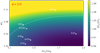Fig. 6 Stationary spin map predicted by our analytical model (Eq. (16)) for a CB planet in the gaseous regime (γ2 ≫ n2) and in an orbit with α = a1∕a2 = 1∕3, as a functionof its eccentricity e2 and the binary mass ratio m1∕m0. The white curve indicates the perfectly synchronous state ⟨Ω2⟩∕n2 = 1. The white dots represent the positions of the Kepler CB planets in this diagram where the gaseous component is expected to be large and located close to the binary.

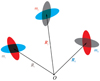Fig. 7 Sketch of the 3BP considering all the tidal interactions between pairs of bodies. The grey, red, and blue ellipsoids are induced on the companions because of the presence of mi, mj, and mk, respectively.

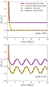Fig. 8 Rotational evolution of a CB planet with the CTL model of Mignard (1979) (Eq. (29)). The initial conditions were taken from Table 1, with the exception of the initial planetary eccentricity (e2 (0) = 0.05 in the upper panel and e2(0) = 0.15 in the bottom panel). Full-line curves indicate the results of filtered numerical integration: excluding the cross tides (in yellow) and considering the full expression (in magenta). Dashed-line curves represent the results of different analytical models: our previous CTL tidal model (Zoppetti et al. 2019) in brown, and the results of the analytical creep tidal model presented in Eq. (16) of this work, expanded up to second-order in α and considering the gaseous limit (γ2 ≫ n1, n2), are shown in grey.

6 Summary and discussion

In this work, we present a model for treating the tides in the general 3BP, in the case in which all the bodies are considered extended and tidally interacting. In particular, we consider the planar case where all the bodies have spin vectors pointing in a direction perpendicular to the orbital plane. We use the creep tide formalism first presented by Ferraz-Mello (2013) to compute the tidal forces and torques, and to study the rotational evolution of a circumbinary planet. The polar flattening due to the rotation of the bodies is also naturally taken into account in the theory (Folonier et al. 2018).

First, we present the creep differential equations that govern the rotational evolution of the extended bodies in the framework of the 3BP. We show that, on each body, the tidal interactions due to the presence of the two companions can be modelled by an equivalent unique interaction. This allows the formalism to be extended to the general N-bodies tidally interacting case, where the difficulty lies in finding the parameters of the equivalent interaction. As in the 2BP, the physical quantities that characterise the rotational evolution of each body in this model are the spin velocities, the equivalent lag-angles, tidal flattenings, and polar flattenings.

We then use the model to study the rotational evolution of a circumbinary planet, taking a Kepler-38-like system (Orosz et al. 2012a) as a working example. To this end, we take advantage of the adiabatic nature of the rotational evolution compared to the orbital evolution in this problem, which lets us assume fixed the orbital elements with the exception of the fast angles.

Using direct numerical integrations, we find that, for planets with low orbital eccentricity and viscosities in the range of the ones estimated for Solar System planets by Ferraz-Mello (2013), the most probable final stationary state is a 1:1 spin–orbit resonance, with the equivalent lag-angle oscillating around zero. The required timescales for reaching the stationary state depend on the relaxation factor of the bodies: taking the relaxation factors estimated for Ferraz-Mello (2013) as a reference, we expect that CB stiff planets in a Kepler-38-like system synchronise their spins within much shorter timescales than the age of the system, while this is not necessarily the case for planets with a large gaseous component. However, the great uncertainty regarding the internal structure of exoplanets, and moreover their associated viscosities, prevents us from calculating an accurate estimate of their rotational evolution timescale.

The high probability of capture in the 1:1 spin–orbit resonance for CB planets with low orbital eccentricity and arbitrary viscosities, motivated us to study this particular solution in more detail. With this aim, we search for a high-order analytical expression for the mean solution of the rotational stationary state. The extreme proximity of Kepler CB planets to their central binary, as seen in evidenced by observations, in addition to the strong dependence of tidal effects with the relative distance between thebodies, motivated us to develop a high-order model in semimajor axis ratio. Our solution has shown to be very precise in predicting the full numerical integrations, for arbitrary planetary viscosity and very high α-values, even inside the expected gravitationally instable region.

From a practical point of view, when studying long-term tidal evolution, having a secular approximation of the stationary rotational solution considerably accelerates the numerical simulation of the full system, avoiding the need to integrate the rotational evolution and, instead, introducing an analytical recipe for the equilibrium state. This semi-analytic method is particularly useful in the case of working with gaseous bodies with large relaxation factors, for which the creep equation becomes particularly difficult to solve efficiently.

As an application of our analytical model, we consider the Kepler CB planets observed close to the central binary and with an expected large gaseous component. If we assume that all these CB planets have viscosities that have caused them to reach their rotational steady state at the present epoch, our model predicts that their typical rotation speeds are subsynchronous. This result is mainly due to the presence of a central binary (instead of a single star) and is predicted by our model for CB planets (i) with very low orbital eccentricity (ii) close to a binary with a high mass ratio. However, the stationary rotation for gaseous CB planets predicted bythe creep tide theory presented here is different from the one expected with the CTL model presented in Zoppetti et al. (2019, 2020).

To explain this discrepancy, we finally discuss the results obtained for the stationary spin of a CB planet with the creep tide theory (in the gaseous limit) and compare with those obtained using the CTL tidal model in Zoppetti et al. (2019, 2020). We show that both models predict exactly the same solution as long as the cross torques are taken into account in the CTL formalism. These torques had been neglected in our previous works, in reaction to studies of the classical case of a single extended body with a system of coordinates attached to it. However, for the general case of extended 3BP and an arbitrary reference frame, these torques cannot be neglected. One of the main advantages of the creep tide theory over the CTL model is the treatment of cross torques. While in the CTL model, the general expressions for the tidal force and torques are very complex and only valid for small and constant time-lags, in the creep theory these quantities are calculated from the equilibrium figures where the cross torques are naturally taken into account.

In addition to this, the CTL model seems to be contained within the creep tide theory, for the case of relaxation factors much higher than the fundamental frequencies of the system. Moreover, in the creep tide formalism the lag-angle is not an external ad-hoc quantity that needs to be small and constant, but can take large values and its temporal evolution is solved from a differential equation. Finally, among its most interesting advantages, we highlight the fact that the calculation of an equivalent equilibrium figure allows not only to take into account the cross torques in a natural way but also to incorporate some additional physical phenomena such as polar flattening. As a result, the theory also provides the evolution of the geometric shape of the interacting bodies.

Among its main limitations, we find some difficulty in numerically solving the creep equation for gaseous bodies with high relaxation factors in an efficient way. This means that, when studying long-term tidal evolution, some analytical recipes need to be incorporated to accelerate the numerical integrations, such as the mean values that describe the rotational evolution presented in this work. On the other hand, as discussed in Ferraz-Mello (2015b), the creep theory is analogous to those theories that consider the extended masses as Maxwell bodies (Correia et al. 2014), but without taking into account the elastic component of the tides. More complex rheologies such as the Sundberg-Cooper model (Sundberg & Cooper 2010) may be necessary to reproduce many of the intricacies seen in the deformation of real materials (e.g. Renaud & Henning 2018).

Acknowledgements

This research was funded by CONICET, SECYT/UNC, FONCYT and FAPESP (Grant 2016/20189-9 and 2016/13750-6. The authors also wish to thank the anonymous referee for helpful suggestions that greatly improved this work).

Appendix A Sixth-order terms for the mean stationary solution

The non-eccentric terms expanded up to sixth order in α of expressions (16)–(19) are respectively given by $$\begin{array}{ll}{\langle {\Omega }_2\rangle }_{o6}=\hfill & -\frac{5{\mathcal{M}}_2(n_1-n_2){\gamma }_2^2{\alpha }^6}{32\left({\gamma }_2^2+{(n_1-n_2)}^2\right)\left({\gamma }_2^2+{(2n_1-2n_2)}^2\right)\left({\gamma }_2^2+{(3n_1-3n_2)}^2\right)}\hfill \\ \hfill & \times [5(121{\gamma }_2^4+805{\gamma }_2^2{(n_1-n_2)}^2+744{(n_1-n_2)}^4){\mathcal{M}}_4\hfill \\ \hfill & -(729{\gamma }_2^4+5265{\gamma }_2^2{(n_1-n_2)}^2+4836{(n_1-n_2)}^4){\mathcal{M}}_2^2]\hfill \end{array}$$(A.1) $${\langle {\delta }_2\rangle }_{o6}=\frac{{\langle {\Omega }_2\rangle }_{o6}}{{\gamma }_2}$$(A.2) $$\begin{array}{ll}\frac{{\langle {\mathcal{E}}_2^{\rho }\rangle }_{o6}}{{\overline{ϵ}}_2^{\rho }}=\hfill & \frac{5M_2{\alpha }^6}{256\left({\gamma }_2^2+{(n_1-n_2)}^2\right)\left({\gamma }_2^2+4{(n_1-n_2)}^2\right)\left({\gamma }_2^2+9{(n_1-n_2)}^2\right)}\hfill \\ \hfill & \times [(105{\mathcal{F}}_1+776{\mathcal{F}}_2){\gamma }_2^6+70(21{\mathcal{F}}_1+76{\mathcal{F}}_2){\gamma }_2^4{(n_1-n_2)}^2\hfill \\ \hfill & +(5145{\mathcal{F}}_1+5024{\mathcal{F}}_2){\gamma }_2^2{(n_1-n_2)}^4+378{\mathcal{F}}_1{(n_1-n_2)}^6]\hfill \end{array}$$(A.3) $$\frac{{\langle {\mathcal{E}}_2^z\rangle }_{o6}}{{\overline{ϵ}}_2^M}=\frac{2{\langle {\Omega }_2\rangle }_{o6}}{n_2}+\frac{{\overline{ϵ}}_2^{\rho }}{{\overline{ϵ}}_2^M}\frac{1225}{512}{\mathcal{M}}_2{\mathcal{F}}_1{\alpha }^6$$(A.4)

where $$\begin{array}{lll}{\mathcal{F}}_1=\frac{1+{\beta }^5}{{(1+\beta )}^5};\hfill & \hfill & {\mathcal{F}}_2=\frac{\beta {(1-\beta )}^2}{{(1+\beta )}^4}.\hfill \end{array}$$(A.5)

References

All Tables

All Figures

	Fig. 1 Three-body problem from an inertial frame and from a mi-relative frame.
In the text

Fig. 2 Left: equilibrium figure in the 3BP. Dashed-empty ellipsoids correspond to the static tidal deformations generated by each of the perturbing masses, while the resulting equilibrium figure of mi (Eq. (3)) is shown by a filled grey ellipsoid. The unit vector ${\widehat{r}}_i^{(\text{eq})}$ indicates the orientation of the equivalent equilibrium bulge. Right: real figure in the 3BP. The dark grey filled ellipsoid represents the modelled real figure induced on mi when we take into account the internal viscosity; we note that it is displaced by an angle δi, with respectto the equilibrium figure and also has different flattenings.

In the text

Fig. 3 Rotational evolution due to tides in a Kepler-38-like CB planet (see Table 1), considering different values of planetary relaxation factor γ2, illustrated here with different colours (see legend in the upper left panel). The evolution was calculated by direct numerical integration of Eqs. (7) and (14). The evolution of the planetary spin rate Ω2 is shown in the upper left panel (zoomed around Ω2 ~ n2 in a secondary plot), the lag-angle δ2 in the upper right panel, the equatorial flattening ${\mathcal{E}}_2^{\rho }$ in the lower left panel and the polar flattening ${\mathcal{E}}_2^z$ in the lower right panel. The dashed black line in the upper left panel shows the stationary solution predicted by Zoppetti et al. (2019) with a CTL-based model.

In the text

Fig. 4 Mean rotational speed ⟨Ω2⟩ (upper left panel), mean lag-angle ⟨δ2⟩ (upper right panel), mean equatorial flattening $\langle {\mathcal{E}}_2^{\rho }\rangle$ (lower left panel) and mean polar flattening $\langle {\mathcal{E}}_2^z\rangle$ (lower right panel) as a function of the planetary relaxation factor normalised by the mean motion frequency γ2 ∕n2. The initial conditions for the system were taken from Table 1, but considering different planetary eccentricities, which are shown with curves of different colours as indicated in the upper left panel. Different types of curves represent different methods for obtaining the mean values: full-line curves represent the numerical results, dashed-line curves represent our sixth-order fit, and dotted-line curves represent the results of considering the 2BP with a central mass equal to the sum of the binary components. The vertical grey line in the upper left panel represents the position in the diagram of a solid Earth (Ferraz-Mello 2013) and the large coloured dots represent the final mean value obtained with different γ2 values, from simulations of Fig. 3 captured in the 1:1 spin–orbit resonance: γ2 ∕n2 = 0.1 (orange), γ2∕n2 = 1 (green), γ2∕n2 = 10 (red) and γ2∕n2 = 100 (magenta).

In the text

Fig. 5 Mean rotational speed ⟨Ω2⟩ (first row panels), mean lag-angle ⟨δ2⟩ (second row panels), mean equatorial flattening $\langle {\mathcal{E}}_2^{\rho }\rangle$ (third row panels) and mean polar flattening $\langle {\mathcal{E}}_2^z\rangle$ (last row panels) as a function of the semimajor axis ratio α = a1∕a2, for the case γ2 = 100n2. The initial conditions for the system were taken from Table 1, but considering different planetary eccentricities, shown with curves of different colours (same colour convention as in Fig. 4), and different secondary mass: m1 = 1∕16 m⊙ (first column) and m1 = 1∕4 m⊙ (second column). Different types of curves represent different methods for obtaining the mean values with the same convention as in Fig. 4 but including the fourth-order fit shown with a dot-dashed line. The magenta dots in the right panels represent the final mean value obtained for this relaxation factor from the simulations of Fig. 3.

In the text

Fig. 6 Stationary spin map predicted by our analytical model (Eq. (16)) for a CB planet in the gaseous regime (γ2 ≫ n2) and in an orbit with α = a1∕a2 = 1∕3, as a functionof its eccentricity e2 and the binary mass ratio m1∕m0. The white curve indicates the perfectly synchronous state ⟨Ω2⟩∕n2 = 1. The white dots represent the positions of the Kepler CB planets in this diagram where the gaseous component is expected to be large and located close to the binary.

In the text

	Fig. 7 Sketch of the 3BP considering all the tidal interactions between pairs of bodies. The grey, red, and blue ellipsoids are induced on the companions because of the presence of mi, mj, and mk, respectively.
In the text

Fig. 8 Rotational evolution of a CB planet with the CTL model of Mignard (1979) (Eq. (29)). The initial conditions were taken from Table 1, with the exception of the initial planetary eccentricity (e2 (0) = 0.05 in the upper panel and e2(0) = 0.15 in the bottom panel). Full-line curves indicate the results of filtered numerical integration: excluding the cross tides (in yellow) and considering the full expression (in magenta). Dashed-line curves represent the results of different analytical models: our previous CTL tidal model (Zoppetti et al. 2019) in brown, and the results of the analytical creep tidal model presented in Eq. (16) of this work, expanded up to second-order in α and considering the gaseous limit (γ2 ≫ n1, n2), are shown in grey.

In the text

References

- Correia, A. C. M., Boué, G., Laskar, J., et al. 2014, A&A, 571, A50 [NASA ADS] [CrossRef] [EDP Sciences] [Google Scholar]
- Correia, A. C. M., Boué, G., & Laskar, J. 2016, Celest. Mech. Dyn. Astron., 126, 189 [NASA ADS] [CrossRef] [Google Scholar]
- Doyle, L. R., Carter, J. A., Fabrycky, D. C., et al. 2011, Science, 333, 1602 [Google Scholar]
- Efroimsky, M. 2012, ApJ, 746, 150 [Google Scholar]
- Efroimsky, M. 2015, AJ, 150, 98 [NASA ADS] [CrossRef] [Google Scholar]
- Ferraz-Mello, S. 2013, Celest. Mech. Dyn. Astron., 116, 109 [Google Scholar]
- Ferraz-Mello, S. 2015a, Celest. Mech. Dyn. Astron., 122, 359 [Google Scholar]
- Ferraz-Mello, S. 2015b, A&A, 579, A97 [CrossRef] [EDP Sciences] [Google Scholar]
- Ferraz-Mello, S., Rodríguez, A., & Hussmann, H. 2008, Celest. Mech. Dyn. Astron., 101, 171 [Google Scholar]
- Folonier, H. A., Ferraz-Mello, S., & Kholshevnikov, K. V. 2015, Celest. Mech. Dyn. Astron., 122, 183 [CrossRef] [Google Scholar]
- Folonier, H. A., Ferraz-Mello, S., & Andrade-Ines, E. 2018, Celest. Mech. Dyn. Astron., 130, 78 [Google Scholar]
- Gomes, G. O., Folonier, H. A., & Ferraz-Mello, S. 2019, Celest. Mech. Dyn. Astron., 131, 56 [Google Scholar]
- Holman, M. J., & Wiegert, P. A. 1999, AJ, 117, 621 [Google Scholar]
- Hurford, T. A., Sarid, A. R., & Greenberg, R. 2007, Icarus, 186, 218 [CrossRef] [Google Scholar]
- Hut, P. 1981, A&A, 99, 126 [NASA ADS] [Google Scholar]
- Kostov, V. B., McCullough, P. R., Carter, J. A., et al. 2014, ApJ, 784, 14 [NASA ADS] [CrossRef] [Google Scholar]
- Lambert, J. D. 1991, Numerical Methods for Ordinary Differential Systems: the Initial Value Problem (Hoboken: John Wiley & Sons) [Google Scholar]
- Makarov, V. V., & Efroimsky, M. 2013, ApJ, 764, 27 [Google Scholar]
- Meriggiola, R. 2012, PhD thesis, The Determination of the Rotational State of Celestial Bodies, La Sapienza, Roma, Italy [Google Scholar]
- Mignard, F. 1979, Moon Planets, 20, 301 [Google Scholar]
- Mills, S. M., & Mazeh, T. 2017, ApJ, 839, L8 [NASA ADS] [CrossRef] [Google Scholar]
- Murray, C. D., & Dermott, S. F. 1999, Solar System Dynamics, eds. C. D. Murray, & S. F. McDermott (Cambridge, UK: Cambridge University Press) [Google Scholar]
- Orosz, J. A., Welsh, W. F., Carter, J. A., et al. 2012a, ApJ, 758, 87 [Google Scholar]
- Orosz, J. A., Welsh, W. F., Carter, J. A., et al. 2012b, Science, 337, 1511 [Google Scholar]
- Renaud, J. P., & Henning, W. G. 2018, ApJ, 857, 98 [Google Scholar]
- Schwamb, M. E., Orosz, J. A., Carter, J. A., et al. 2013, ApJ, 768, 127 [Google Scholar]
- Socia, Q. J., Welsh, W. F., Orosz, J. A., et al. 2020, AJ, 159, 94 [Google Scholar]
- Sundberg, M., & Cooper, R. F. 2010, Philos. Mag., 90, 2817 [Google Scholar]
- Tisserand, F. 1891, Traité de mécanique céleste (Paris: Gauthier-Villars) [Google Scholar]
- Welsh, W. F., Orosz, J. A., Carter, J. A., et al. 2012, Nature, 481, 475 [Google Scholar]
- Zoppetti, F. A., Beaugé, C., & Leiva, A. M. 2018, MNRAS, 477, 5301 [Google Scholar]
- Zoppetti, F. A., Beaugé, C., Leiva, A. M., et al. 2019, A&A, 627, A109 [NASA ADS] [CrossRef] [EDP Sciences] [Google Scholar]
- Zoppetti, F. A., Leiva, A. M., & Beaugé, C. 2020, A&A, 634, A12 [EDP Sciences] [Google Scholar]
All Tables
Initial conditions of our reference numerical simulation, representing a Kepler-38-like system (Orosz et al. 2012a).