| Issue |
A&A
Volume 651, July 2021
|
|
|---|---|---|
| Article Number | A106 | |
| Number of page(s) | 18 | |
| Section | Stellar structure and evolution | |
| DOI | https://doi.org/10.1051/0004-6361/202140769 | |
| Published online | 28 July 2021 | |
Standard solar models: Perspectives from updated solar neutrino fluxes and gravity-mode period spacing
1
Observatoire de Genève, Université de Genève, Ch. Pegasi 51b, 1290 Sauverny, Switzerland
e-mail: This email address is being protected from spambots. You need JavaScript enabled to view it.
2
STAR Institute, Université de Liège, Allée du 6 Août 19C, 4000 Liège, Belgium
Received:
9
March
2021
Accepted:
27
April
2021
Abstract
Context. Thanks to the vast and exquisite set of observations that have been made available for the Sun, our star is by far an ideal target for testing stellar models with a unique precision. A recent issue under consideration in the field is related to the progress in the solar surface abundances derivation that has led to a decrease of the solar metallicity. While the former high-metallicity models were in fair agreement with other observational indicators from helioseismology and solar neutrino fluxes, it is no longer the case for low-metallicity models. This issue has become known as ‘the solar problem’. Recent data are, however, promising to shed a new light on it. For instance, in 2020, the Borexino Collaboration released the first-ever complete estimate of neutrinos emitted in the CNO cycle, which has reaffirmed the role of the neutrino constraints in the solar modelling process and their potential in exploring related issues. In parallel, a newly claimed detection of solar gravity modes of oscillation offers another opportunity for probing the stratification in the Sun’s central layers.
Aims. We propose combining the diagnoses from neutrinos and helioseismology, both from pressure and gravity modes, in assessing the predictions of solar models. We compare in detail the different physical prescriptions currently at our disposal with regard to stellar model computations.
Methods. We build a series of solar standard models based on a variation of the different physical ingredients directly affecting the core structure: opacity, chemical mixture, nuclear reactions rates. We compare the predictions of these models to their observational counterparts for the neutrinos fluxes, gravity-mode period spacing, and low-degree pressure mode frequency ratios.
Results. The CNO neutrino flux confirms previous findings, exhibiting a preference for high-metallicity models. Nevertheless, we find that mild modification of the nuclear screening factors can re-match low-metallicity model predictions to observed fluxes, although it does not restore the agreement with the helioseismic frequency ratios. Neither the high-metallicity or low-metallicity models are able to reproduce the gravity-mode period spacing. The disagreement is huge, more than 100σ to the observed value. Reversely, the family of standard models narrows the expected range of the Sun’s period spacing: between ∼2150 and ∼2190 s. Moreover, we show this indicator can constrain the chemical mixture, opacity, and – to a lower extent – nuclear reactions in solar models.
Key words: Sun: interior / opacity / nuclear reactions, nucleosynthesis, abundances / Sun: helioseismology / neutrinos
© ESO 2021
1. Introduction
The Sun is a prodigious testbed for the field of stellar physics. We benefit from a privileged view into its internal structure thanks to solar oscillation (helioseismic) observations and solar neutrino detections, while we can estimate its envelope composition from spectroscopic determinations of element abundances at its surface.
Helioseismology has precisely constrained the Sun’s convective envelope and neighbour superficial radiative regions (see e.g. recent reviews by Buldgen et al. 2019; Christensen-Dalsgaard 2021, and references therein). In a non-exhaustive list, we can highlight: the determination of the location of the base of the convective envelope (Kosovichev & Fedorova 1991; Christensen-Dalsgaard et al. 1991), the reconstruction of the internal rotation profile, and the highlighting of the tachocline (e.g. Kosovichev 1988; Brown et al. 1989; Schou et al. 1998), as well as the determination of the helium abundance in the convective envelope (Vorontsov et al. 1991; Basu & Antia 1995) and seismic inversions of the sound speed profile (Christensen-Dalsgaard et al. 1985), along with other structural variables (see reviews by Christensen-Dalsgaard 2002; Kosovichev 2011; Basu 2016, and references therein).
In parallel, the constant improvement of detectors of neutrinos from extra-terrestrial sources, in particular, those intended to detect neutrinos of solar origin (initiated decades ago, see Davis et al. 1968), has forged a new path to constraining the physical conditions and nuclear burning in the Sun’s central layers (e.g. including reviews, Bahcall & Ulrich 1988; Turck-Chièze & Couvidat 2011; Haxton et al. 2013). The potential of solar neutrino measurements has been confirmed by supporting evidences for neutrino oscillation (e.g. Bahcall et al. 1998; Fukuda et al. 1999) as well as binding solar central temperatures, opacities, abundances, or nuclear reaction rates (e.g. Turck-Chieze & Lopes 1993; degl’Innocenti et al. 1998; Watanabe & Shibahashi 2001; Antia & Chitre 2002; Gonzalez 2006; Serenelli et al. 2013; Serenelli 2016). Interestingly, these central temperatures can be compared to those estimated from seismic models (e.g. Antia & Chitre 1995, 1998; Ricci & Berezinsky 1997), and reveal potential flaws in the standard solar models.
Despite these successes, solar physics now faces a stalemate. The chemical element abundances composing the solar plasma are an obvious key ingredient for computing a model of the Sun. They are taken as the Sun’s surface composition, derived by spectroscopic analysis of its photosphere. In 2005, new 3D atmosphere simulations and better atomic data led to a downward revision of the most abundant elements, C, N, O, and Ne, by ∼30% (Asplund et al. 2005, hereafter AGS05). The solar metallicity decreases in revised determinations (AGS05; Caffau et al. 2011; Asplund et al. 2009, hereafter AGSS09) in comparison to previous ones (e.g. Grevesse & Noels 1993; Grevesse & Sauval 1998). As a consequence, standard solar models (hereafter SSMs), including revised abundances, are no longer in agreement with helioseismology: the base of the convective envelope is too shallow, the helium surface abundance is lower than the helioseismic one, and the results of inverse methods for acoustic variables present larger differences with the Sun’s acoustic structure (Montalbán et al. 2004; Turck-Chièze et al. 2004; Bahcall et al. 2005; Antia & Basu 2005; Guzik et al. 2006; Serenelli et al. 2009). Rapidly, possible solutions or expected improvements to this issue were thus proposed; see, for instance, Basu & Antia (2008) and Guzik & Mussack (2010). These include opacity underestimation, accretion by young Sun, overshooting, etc.
Comparisons to solar neutrino fluxes similarly show that the SSMs are divided into two categories according to the adopted chemical mixture; the high-metallicity ones (old solar abundance determinations) are favoured as they better predict the rates of production of solar neutrinos than those of low metallicity (revised solar abundances), see e.g. works by Bergström et al. (2016) and Vinyoles et al. (2017). This result relies in particular on the analysis of Φ(Be) and Φ(B), the respective neutrinos fluxes produced by the 7Be electronic capture in the ppII branch, and the β decay of 8B in the ppIII branch (subchains of the pp H-burning process).
However, we can now count on precision improvement and new observational constraints for shedding a new light on these issues. At first, the Borexino Collaboration (2020) has improved greatly the determination of neutrino fluxes from the CNO cycle, and gave for the first time an estimate of the fraction of nuclear energy generated by CNO in the Sun. Recently, Fossat et al. (2017) announced the detection of solar gravity (g) modes from the analysis of 16.5 year-long data series of the GOLF instrument dedicated to helioseismology (Gabriel et al. 1995), on board of the SOHO satellite. Besides constricting rotation in deeper layers of the Sun than pressure (p) modes, the period spacing of the g modes, a nearly constant value, is sensitive to the stratification at the centre (e.g. Berthomieu & Provost 1991). However, a series of works (Schunker et al. 2018; Appourchaux & Corbard 2019; Scherrer & Gough 2019) puts serious doubts on this recent detection, which is now more than weakened. But given the potentially reachable precision on the period spacing with the methods used in Fossat et al. (2017) and Fossat & Schmider (2018), exploring the way the latter can constrain solar models remains of interest (see e.g. comparison with estimates from seismic models in Buldgen et al. 2020).
We show how a firm detection of the period spacing in combination with the most recent solar neutrinos constraints would be strongly complementary to the exploration of the central physical conditions of the Sun. We also use information on the innermost regions that can be given by solar p-modes, through their combination as frequency ratios (see Roxburgh & Vorontsov 2003; Chaplin et al. 2007). We compare these indicators with a series of SSMs for which the physics is varied, following: chemical mixture, opacity, nuclear reaction rates, microscopic diffusion. These standard inputs are the factors that affect the conditions at the Sun’s core most, and so they are the most sensitive to exploration with the observational data set proposed above. As we have set focus on central layers of models, the outer envelope layers will not necessarily be in agreement with all of the helioseismic indicators.
We start in Sect. 2 by presenting the different solar observational constraints considered in this paper. We then describe the series of standard solar models and their different input physics in Sect. 3. We check their consistency with g-mode spacing, neutrino fluxes, and frequency ratios of low-degree p modes in Sect. 4. We discuss the accuracy of the results in Sect. 5 and we present our conclusions in Sect. 6.
2. Observational neutrino fluxes, gravity-mode period spacing, and pressure-mode frequency ratios
The measurement of neutrinos produced by the Sun provides information on the thermal structure at its centre. There, the neutrino production is a function of the nuclear reaction rates, the chemical abundances (and plasma density), and temperatures. Considering the neutrino fluxes predicted by a SSM, they not only depend on the choice of the nuclear reaction rates and element abundances, but also on the parameters affecting the thermal structure. This model structure itself depends on the nuclear reaction rates and abundances, but also the opacity and to a lower extent, the equation of state. In this way, it lists the essential physical ingredients of solar models that neutrinos afford to test.
2.1. Solar neutrino fluxes
The solar neutrino fluxes Φ that can be determined using terrestrial experiments are related to the following nuclear reactions and electronic captures/disintegrations, parts either of the pp chain or the CNO cycle:
 (1)
(1)
 (2)
(2)
 (3)
(3)
 (4)
(4)
 (5)
(5)
 (6)
(6)
 (7)
(7)
 (8)
(8)
For the isotopes implied in the reactions constituent of the CNO cycle (Eqs. (4)–(6)), neutrino production is also made possible via electronic capture. The latter is not included in the computation of our SSMs, but it has no impact on the prediction of neutrino production rates since electronic captures occur less frequently than β decays by several orders of magnitude (see e.g. Stonehill et al. 2004).
The observational constraints for the neutrino fluxes are summarised in Table 1. The results of two distinct analyses are taken into consideration. At first, those obtained by (Bergström et al. 2016, hereafter B16), in which the authors carried out a statistical analysis of a large collection1 of solar neutrino experiments; data taken from cumulative experiment based on Cl or Ga detectors (Homestake, Gallex/GNO, SAGE), and from real-time detectors Super-Kamiokande (4 campaign phases), SNO (3 phases) and Borexino (2 phases). Excepting the evident dependence on neutrino oscillations parameters, the B16 approach is almost model-independent (see also the details in Bahcall 2002). We selected in particular the set of fluxes that these authors derived with the solar luminosity as a constraint since it does not induce a dependence on solar models. The solar radiative luminosity measurement is indeed independent of the solar model and, for instance, B16 adopted that of Fröhlich & Lean (1998), L⊙ = 3.842 × 1033 erg s−1. Using the luminosity reduces the uncertainties on fluxes, in particular on Φ(Be) and Φ(B), as the energy per reaction produced by the ppII and ppIII branches is much larger than the ppI one (which is however dominant by the number of reactions going through this branch).
Solar neutrino fluxes at 1 AU from the combined analysis of B16 and from the Borexino Collaboration (2018, 2020).
We present the second set in Table 1, which are the fluxes reported by the Borexino Collaboration. The Borexino experiment is highly sensitive to low-energy neutrino and the Collaboration did an intense effort to identify and reduce sources of background contamination. It led to a series of advances: the first measurement of Φ(Be) and the direct evidence of Φ(pp), including the measurement of its spectra. Finally, it recently provided the first direct measurement of the neutrinos produced by the CNO cycle (Eqs. (4)–(6)). In comparison to B16, where not all of the Borexino campaigns were included, the latest results of the Borexino Collaboration (2018, 2020) rely on a greater store of data. The results of this Collaboration are of interest with regard to comparisons with SSMs, as, in addition to refined Φ(pp), Φ(Be) and Φ(B) values, they provide an absolute estimate for Φ(CNO).
The Borexino results show a significant difference for Φ(B), namely, the value is 10% larger than in the B16 analysis. Although the two sets agree within 1σ due to the large errors in the Borexino set, the change in the estimation of Φ(B) could impact the comparison with theoretical solar models. Moreover, as specified in B16, the derivation of Φ(8B) is almost insensitive to the solar luminosity constraint. The comparison with results from other experimental facilities confirms that the Borexino measurement for Φ(8B) gives the highest estimated value. For instance, it exceeds by ∼8% that of the two other recent neutrino experiments, SNO (Aharmim et al. 2013) and Super-Kamiokande (Abe et al. 2016), although they remain all in agreement to the 1σ level.
We did not use the Φ(pep) observational determination (e.g. Bellini et al. 2012) for comparisons with our SSMs. The pep reaction (Eq. (7)) is an alternative branch to the p+p production of deuteron (Eq. (1)). The pep reactions are not included in the nuclear network of our stellar models in reason of their marginal contribution to the total pp-chain energy production. If included in solar models (e.g. B16), only ∼0.6% of 2H appear to be created through pep channel. Moreover, the pep reaction rate shares the same nuclear matrix elements as that of the p+p reaction, so that the pep is expressed as a function of the p+p rate (see Adelberger et al. 2011). It would not be actually an independent constraint, as it would rely on an estimate of the p+p reactions in our models.
Similarly, we did not include Φ(hep) when testing the SSMs in Sect. 4. Although the hep proton capture (Eq. (8)) generates the most energetic neutrinos, and which are experimentally accessible, the probability of pp chain to go trough this reaction is very low (∼10−5) and this is not included in our nuclear network. The hep reaction cross-section is difficult to compute, as it is only accessible by theoretical mean. It suffers from a large uncertainty (large in comparison to the other reactions involved in H burning) of ∼30% (Adelberger et al. 2011), so its usefulness in the study of the structure of SSMs is negligible.
2.2. Helioseismic indicators
The information offered by oscillation modes is a function of acoustic quantities (e.g. the sound speed, c) that differ according to the nature of the modes. They are not directly sensitive to the thermal structure, as is the case for the neutrino constraints. Combining these indicators thus provides access to the solar structure and its associated physics under complementary views.
The natural complement for probing central solar regions would be the knowledge of gravity modes. They generally propagate in the central regions of stars, but given the extended evanescent region constituted by the convective envelope, the g-modes are expected to be of very low amplitude at the solar surface. Thus, detecting them poses a significant challenge (see review by Appourchaux et al. 2010). Claims of solar g-mode discoveries have been made in the past (Severnyi et al. 1976; Delache & Scherrer 1983; García et al. 2007) but have since been questioned or have remained unconfirmed (see detailed chronological review by Appourchaux & Pallé 2013). More recently, (Fossat et al. 2017, hereafter Fo17) (see also Fossat & Schmider 2018) announced another detection of this long-awaited helioseismic missing link. Fossat et al. (2017) present what would correspond to the signatures, each a hundred modes apiece, of asymptotic g-modes of angular degrees ℓ = 1 and ℓ = 2. With the rotational splittings that they determine, the core rotation of the Sun would be ∼3.8 higher than that of the envelope.
For the first time, Fo17 also provided a precise estimation of the asymptotic period spacing P0 = 2041 ± 1 s, also given in Table 1. The almost constant value in period between g-modes of same ℓ and consecutive radial orders n is well approximated at a first order by the asymptotic period spacing, P0, providing a factor of  . Following asymptotic developments (Provost & Berthomieu 1986; Ellis 1986), the P0 for the Sun can be expressed in good approximation as:
 (9)
(9)
where rc is the location of the base of the convective zone, N the Brunt–Väisälä frequency, and r the radius. The central layers weigh the more in the integral in reason of the variation in 1/r. The P0 is thus a good marker of the chemical stratification of the core region, since N takes its largest values in layers with marked chemical composition gradients and it has appeared early on as a candidate for characterising the innermost regions of solar models (e.g. Berthomieu & Provost 1991).
The detection by Fo17 is put into doubt (Schunker et al. 2018; Scherrer & Gough 2019; Appourchaux & Corbard 2019). Early results from a series of seismic models derived by Buldgen et al. (2020) confirm a strong disagreement between the values predicted by these models and the Fo17 observational one. All this leads to the conclusion that the detection cannot be relied on. However, Fo17 reported its value with a high precision of ∼0.05%. We hence compared that period spacing with SSMs to confirm its disagreement with solar models (in the wake of preliminary results by Buldgen et al. 2020), whatever the physics used. But we also verify whether, in combination with neutrino fluxes and assuming such a potential precision, the P0 helps discriminate SSMs with different physics and, in particular, between high- and low-metallicity ones.
The well-confirmed solar p-modes can also be combined to define seismic indicators sensitive to deeper solar regions. Roxburgh & Vorontsov (2003) proposed to combine for solar-like stars the small and large frequency separations of low-degree p-modes as:
 (10)
(10)
 (11)
(11)
where Δνn, ℓ = νn, ℓ − νn − 1, ℓ and δνn, ℓ = νn, ℓ − νn − 1, ℓ + 2 are, respectively, the large and small frequency separations, with νn, ℓ as the frequency of the mode of order n and degree ℓ. The frequency ratios r02 and r13 have the advantage to be insensitive to surface effects affecting the p-mode oscillations. These indicators are in particular sensitive to the sound speed in the central stellar layers (Gough 2003), that is on the gradient of chemical composition. They are a useful complement to neutrinos and g-modes in probing the physical conditions in layers at the vicinity of the solar core. Chaplin et al. (2007) extensively explored which physical quantities are probed with their help. They also confirmed, as in Basu et al. (2007), that high-metallicity SSMs were clearly better at reproducing the solar frequency ratios. We naturally include these indicators in this work for the purpose of further testing on an extended series of SSMs, as in the approach in Buldgen et al. (2019). We took the low-degree frequencies from the solar BiSON set (Davies et al. 2014; Hale et al. 2016) to compute the observed ratios.
3. Physics of the standard solar models
We calibrated a series of standard solar models to be representative of the present Sun, following the recipe suggested in Bahcall et al. (1982): we computed the stellar evolution of 1 M⊙ model to the present age of the Sun (4.57 Gyr) imposing to reproduce the Sun’s luminosity and radius, 1 L⊙ and 1 R⊙, as well as the present-day surface metallicity (Z/X)s (relative to X, the hydrogen abundance). This latter quantity depends of course on the compilation of stellar surface abundances adopted. We took for the solar luminosity the value recommended in 2015 by the International Astronomical Union (IAU) in resolution B3, i.e. L⊙ = 3.828 × 1033 erg s−1.
All of our models were computed with help of the Liège stellar evolution code, CLES (Scuflaire et al. 2008a). Convection is treated under the mixing-length theory, implemented as in Cox & Giuli (1968). Excepting explicit mention, we include microscopic diffusion with coefficients derived from the resolution of Burgers’ equations following the method in Thoul et al. (1994). Metals heavier than He are all assimilated as Fe. No convective overshooting was considered.
Unless a change in one of the ingredient is specified, the models adopt nuclear reaction rates from the Adelberger et al. (2011) compilation, FreeEos equation of state (Irwin 2012), OPAL opacities (Iglesias & Rogers 1996) that are supplemented with Potekhin’s electron-conduction opacities (Cassisi et al. 2007), and grey model atmosphere with Eddington’s law for the temperature T(τ) relation, with atmospheres extending up to an optical depth τ = 10−4. The default chemical mixture is that of AGSS09. The opacities are all supplemented at low-temperature conditions by those of Ferguson et al. (2005), adapted to the chemical mixture selected. Finally, the adiabatic frequencies for the computation of frequency ratios are obtained with the Liège oscillation code, LOSC (Scuflaire et al. 2008b).
We describe the physics that we varied in order to calibrate different SSMs below. We briefly review the main differences between datasets of stellar physics at our disposal, as well as the uncertainties that continue to affect them.
Solar chemical mixture. As a result of diffusion processes (Christensen-Dalsgaard et al. 1993), the present-day solar surface composition depends on its past evolution. Therefore, the determination of the initial composition of the Sun stems from solar calibrations, and depending on the set of surface abundances, it will result in different initial values. For instance, calibrations based on older determinations of the Sun’s surface abundances yield high metallicity estimates (Z ∼ 0.017 − 0.020). Those based on more recent abundances give low estimates (Z ∼ 0.013). Among the “old” determinations, the most frequently used are those of Grevesse & Noels (1993, hereafter GN93) and Grevesse & Sauval (1998, hereafter GS98). The consequences of revising of these abundances on the solar structure and its helioseismic constraints has been extensively investigated in Bahcall et al. (2005, 2006), Basu & Antia (2008).
Currently, solar observational neutrino constraints tend to favour the high-metallicity SSMs (B16 Vinyoles et al. 2017; Song et al. 2018), while the helioseismic picture is unclear: frequency ratios are better reproduced by high-metallicity models (Basu et al. 2007), but seismic inversions of metallicity points to lower estimates of the metallicity in the envelope (Vorontsov et al. 2013; Buldgen et al. 2017), in favour of the current determinations of surface abundances. Caution on previous assumptions in the older determinations of solar abundances is also made (e.g. Grevesse et al. 2013). Revised determinations include, in particular, 3D (versus 1D previously) hydrodynamical simulations of the solar atmosphere, thorough review of oscillator strengths for the computation of spectroscopic lines, and appended lists of line blends in solar photospheric spectra. The solar abundances by Asplund et al. (2009, hereafter AGSS09) now appear as a stable reference. The latest updates have not significantly affected the recommended abundance values (Scott et al. 2015; Grevesse et al. 2015; Amarsi et al. 2020), particularly, in the sensitive case of C and N elements (Amarsi et al. 2019, 2020), which are among the highest abundant metals and, thus, impacting the metallicity.
Meanwhile, Caffau et al. (2011, hereafter Caffau11) carried out an independent determination of solar abundances. The authors restricted their analysis to a lower number of surface abundances, focusing on the most abundant elements. The solar metallicity they obtained is between that of GS98 and AGSS09.
Among the most abundant metals, the determination of Ne abundance falls apart since it cannot be derived from spectroscopy of the photosphere. Determined from quiet regions in the solar corona, recent studies by Landi & Testa (2015) and Young (2018) recommend an increase in [Ne/O] (neon-to-oxygen abundance) by 40%. Neon contributes significantly to the opacity in solar radiative regions (see an illustration of its contribution to solar opacities in Blancard et al. 2012). It is hence worth combining the AGSS09 set with the recommended increase in the Ne abundance; we refer to this mixture as AGSS09+Ne. As a summary, we compared the role of the chemical mixture with help of SSMs calibrated with: GN93, GN98, Caffau11, AGSS09, and AGSS09+Ne.
Opacity. The two opacity libraries mostly used in stellar models are those of the OPAL (Iglesias & Rogers 1996) and OP (Badnell et al. 2005) projects. In the solar case, attention was drifted on differences between the opacity datasets at conditions corresponding to the base of the convective zone (BCZ). Seaton & Badnell (2004) show these differences, which rise to ∼5% at the BCZ (log T ∼ 6.3), find their origin in the equations of state internal to the opacity codes (OPAL predicting more metals in excited states than OP).
On the quest for solving the solar problem created by the revision of metallicity, the accuracy of theoretical opacity data at solar conditions was seriously questioned by Bailey et al. (2014). In an experimental set-up on the Sandia Z-pinch machine, they reproduced conditions of ionisation and temperature of the BCZ and measured a much larger iron spectral opacity than predicted by theoretical opacity computations. The source of the discrepancy received a lot of attention, see, for instance, Iglesias (2015), Pain & Gilleron (2015), or Nahar & Pradhan (2016). Additional experimental campaigns at Sandia have shown other discrepancies with theoretical spectral opacities for iron-group elements Cr and Ni (Nagayama et al. 2019). An explanation with regard to these opacity issues is still pending. However, it has led to an effort for renewed improvement of stellar opacities. The Los Alamos group used their newly developed equation of state and their own set of atomic computations to release the OPLIB opacity library, which was specially designed for stellar evolution codes (Colgan et al. 2016). Despite restricted to tighter ranges of density and temperature conditions, the OPAS dataset (Mondet et al. 2015) covers enough ranges of parameters for computation of solar models (Le Pennec et al. 2015). OP, OPAL, and OPAS tables present differences of a few percent in the radiative solar regions, likely due to the internal equations of state of the different codes; OPLIB stands out by much lower opacities, ∼10 − 15% in comparison to the other tables. It leads OPLIB to impact considerably the temperature gradient of the radiative region. This is expected to penalise the neutrino fluxes predicted by OPLIB SSMs (Song et al. 2018). We explore the role of opacity by calibrating a series of four SSMs with all the opacity tables currently at our disposal; OPAL, OP, OPLIB, and OPAS.
Nuclear reaction rates. The methods for computing astrophysical S-factors require complex nuclear computations; either for extrapolating results of experiment measurement (which cannot access energy domain of nuclear reactions in stars), with an analysis of systematics and other sources of experimental errors, or for deriving them completely ab initio when no experiment is feasible at all. Detailing the uncertainties affecting the S-factor determinations is out of the scope of this paper and we refer to the thorough review of that subject by Adelberger et al. (2011), also referred as the SF-II (Solar Fusion) project. Their work considered a whole set of nuclear reactions of stellar interest and is complete for those involving hydrogen burning. The S-factors of this compilation are of practical use for stellar computations and we selected them as the default choice for the calibration of our SSMs. We also calibrated two SSMs with help of the Nuclear Astrophysics Compilation of REaction (NACRE) rates. One calibration was made with the NACRE rates (Angulo et al. 1999), excepting the 2N(p,γ)15O reaction, which follows the revision by Imbriani et al. (2005; see detail below). Although it has been updated in the meantime, NACRE was used in many stellar models, and we thus find it interesting to confront it with solar data. We eventually considered the updated rates of the project, known as the NACRE II compilation (Xu et al. 2013), which includes the experimental results published in the interval of the NACRE publication. It also follows a distinct method than the results of R-matrix computations presented in Adelberger et al. (2011). The NACRE II authors extrapolate, on their own, the S-factors at low-energy following one systematic approach, based on the potential model method.
We briefly mention the estimated orders of uncertainties affecting the rates of the reactions involved in the production of neutrinos considered in this work (Eqs. (1)–(6)). These uncertainties are discussed in detail in Vinyoles et al. (2017), which also include results obtained posteriorly to the reviews mentioned above.
The p+p reaction (Eq. (1)) can only be determined via an ab initio computation. The details of these are nowadays well understood, and the error on the S11 factor is estimated to be ∼1% (Adelberger et al. 2011). According to (Vinyoles et al. 2017, and references therein), the errors on S17 – the reaction producing 8B isotopes, source of Eq. (2) – is ∼5%. In the CNO cycle, details of the 14N(p,γ)15O reaction are crucial. The reaction is the slowest and represent a bottleneck for the cycle when at equilibrium; most of the isotopes are then under the form of 14N. Experimental measurements at the LUNA accelerator (e.g. Formicola et al. 2004; Marta et al. 2008) recently led to an important reassessment of the S114 factor. Meanwhile the value recommended by SF-II, further measurements were conducted at LUNA (Marta et al. 2011). This latter suggests a decrease of ∼6% of the S114 factor, while taking into account the errors, the results based on previous LUNA campaigns remain in good agreement. Besides, the different computational method used by NACRE II also leads to a difference of ∼8% with SF-II.
Screening effects -due to the free electron cloud reducing the Coulomb barrier between nuclides- are treated following the weak-screening formalism of Salpeter (1954). Various criticisms on the accuracy of this formalism have been made (e.g. Dzitko et al. 1995; Shaviv & Shaviv 2001), although to which extent it can affect screening factors is a matter of debate (Gruzinov & Bahcall 1998; Bahcall 2002). The development of an advanced formalism accounting for them is a hard task. The potential role of dynamical effects in the screening computation has in particular been advanced by Shaviv (2004). Preliminary attemps to include them confirm they can alter the values of the screening factor (e.g. Mao et al. 2009; Mussack & Däppen 2011; Wood et al. 2018). Estimation of the uncertainties associated to the non-inclusion of dynamical effects in screening factors shows they could go up to 4 − 5% for some of the reactions in the pp chain (Shaviv 2007, 2010). As screening effects play the role of a catalyst on nuclear reactions, we evaluated the impact of uncertainties by implementing parametric changes of the screening factors in Sect. 4.3.
Microscopic diffusion. The surface metallicity along the stellar evolution of a solar model is obviously altered by diffusion. Since this metallicity is used to constrain the calibration of SSMs, the prescription of microscopic diffusion plays an important evolutionary effect on the resulting model. It also acts on a structural side, by affecting the mean molecular weight under the convective region. All our SSMs include microscopic diffusion based on Thoul et al. (1994) as mentioned above. In this approach, the perfect gas equation is assumed valid and the stellar plasma is considered as completely ionised. However, these hypotheses are not entirely appropriate for the whole solar interior, especially at low temperatures, and it can lead to overestimation of diffusion coefficients. To estimate this impact, we did a calibration that includes collision integrals in the diffusion coefficients, as proposed by Paquette et al. (1986), accounting for departures to perfect gas conditions. In that case, oxygen was taken as the mean representative of metals.
Equation of state. In first approximation, the equation of state in central radiative layers should be that of a perfect gas, with an adiabatic index Γ1 = ∂lnP/∂lnρ|S ≃ 5/3, where P, ρ, S are respectively the pressure, density and entropy. However, helioseismic inversions of this index revealed small departures of ∼0.1−0.2 % in the deepest layers of the Sun, which are due to relativistic effects (Elliott & Kosovichev 1998). While these departures to the perfect gas are likely to have negligible impact on neutrino production, they affect helioseismic indicators. We tested various equations of state derived following the ‘chemical’ picture, a method based on the minimisation of the free-energy. Approximations at certain levels of the computations (e.g. the effect described above) can drive differences between the equations of state derived following that approach. In addition to FreeEOS, used as reference, we did calibrations with the CEFF (Eggleton et al. 1973; Christensen-Dalsgaard & Daeppen 1992), and SAHA-S (Gryaznov et al. 2004; Baturin et al. 2013) equations of state. We also computed one SSM with the OPAL equation of state (Rogers & Nayfonov 2002), which follows the ‘physical’ picture, i.e. a formalism describing the plasma elements with their fundamental constituents and based on ab initio wavefunction computations.
4. Comparison of model predictions with observations
We present in this section the predictions of the SSMs calibrated with the different physics aforementioned. For comparison with the two sets of observational neutrinos fluxes considered, we computed the reduced χ2 functions:
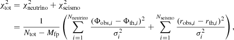 (12)
(12)
where Ntot = Nneutrino + Nseismo, the sum of the number of neutrino fluxes and the number of seismic frequency ratios respectively considered. Mfp is the number of stellar parameters let free in the calibration of the SSM. The Φobs and Φtheor are the solar neutrino fluxes observed and predicted by the theoretical SSM; robs and rth are the observed and theoretical frequency ratios (r02 and r13). The σi are the errors associated to the corresponding observed quantities. In the case of the B16 data, we only included Φ(pp), Φ(Be), Φ(B) in the computation of the χ2 function, given the large uncertainties on the fluxes from CNO. We nevertheless accounted for Φ(CNO) in the Borexino case.
We did not take into account P0 in the merit function. As we detail in the following subsections, P0, as determined by Fo17, actually appeared in strong disagreement with the theoretical values of our SSMs.
4.1. Impact of the solar chemical mixture
The core temperature and central abundances, the neutrino fluxes, and the P0 predicted by the SSMs have been calibrated with different mixtures and are presented in Table 2. The immediate result is the confirmation of the extreme disagreement with the P0 value reported by Fo17. As shown in the upper left panel of Fig. 1, the values from the different SSMs range from 2155 to 2178 s, which is larger by more than 100 s, and so 100σ, than that of Fo17. This disagreement is in support of the dispute about this detection (Schunker et al. 2018; Scherrer & Gough 2019; Appourchaux & Corbard 2019; Buldgen et al. 2020). The order of the disagreement is of similar amplitude when changing other physics input in the models (see following subsections). The solar models cannot be used to interpret the nature itself of the signal found by Fo17, but it confirms an issue with the reported value of the period spacing.
 |
Fig. 1. Neutrino fluxes predicted by the standard solar models (see Sect. 3) with different chemical mixtures. The comparison to the observational fluxes derived by B16 is shown in the left panels, and to the Borexino Collaboration in the right panel. Left upper panel: two boxes are inserted to present a zoom on the Φ(pp) and P0 comparisons. In the panel at the bottom, the comparison is restricted to Φ(pp), Φ(Be) and Φ(B) from the B16 set only for the sake of clarity. The 1σ intervals on the observations are shaded in blue in the three panels. The 3σ range is shaded in light blue in the bottom panel. |
Stellar parameters of the SSMs calibrated with different solar chemical mixtures.
Interestingly, the range predicted by these SSMs could reversely serve as a predictive marker for refined search of solar g modes. Furthermore, P0 varies between 10 and 20 s between the SSMs, an order larger than the observational precision offered by the Fo17 method. A confirmed detection of the solar g-mode period spacing would be an additional strong constraint on the central layers. The variations in P0 that we observe in our SSMs find their origin in changes induced on N in the most central layers. In these regions, we can assume, as a good approximation, the plasma as a perfect fully ionised gas, so that the Brunt–Väisälä frequency can be expressed as N ≃ g2(ρ/P)(∇ad + ∇μ−∇T), where g is the local gravity acceleration, ∇ad the adiabatic gradient, ∇μ the gradient of mean molecular weight, and ∇T the temperature gradient.
We consequently checked the profiles of N in the five SSMs with the different adopted solar mixtures. The global shape of N as a function of r does not change significantly. Yet the values of the peak in N close to the centre (r/R ∼ 0.1) do differ; among the terms in the expression of N given above, we identify variation of ∇μ as the largest contributor to change in N and so P0. The central ∇μ increases as the chemical mixture is more metal-rich, leading for the GN93 and GS98 models to a lower P0. The μ gradient appears in reason of the nuclear reactions and the fact their rates present different temperature law dependences. In the case of a change in the chemical mixture, the sharpness of ∇μ is essentially affected by the impact of abundance modifications on the nuclear reactions. This is seen in Table 2 by the variations between SSMs of Xc and Zc, the central mass fraction of H and metals. The only exception concern the difference in P0 between the AGSS09 and AGSS09+Ne models; the change in ∇T is then dominating the changes in N and P0. The effect is not surprising as Ne is a significant contributor to opacity (κ) in the radiative layers of the Sun (e.g. Antia & Basu 2005; Lin et al. 2007).
4.1.1. Comparison to neutrino observations: The B16 set
Recent studies have discussed the chemical mixture impact on neutrino predictions from SSMs and compared them with the B16 observational set. Vinyoles et al. (2017) and Zhang et al. (2019) found the observed values of Φ(pp), Φ(Be) and Φ(B) fall between those predicted by the SSMs that they calibrated with GN98 and AGSS092. The concordance of all their SSMs with these solar fluxes is within 3σ, although the GS98 models are in closer agreement.
However, our results lead to a different picture; our SSMs with AGSS09 and AGSS09+Ne are better than the GN93 or GS98 ones at reproducing the solar fluxes according to the values of  in Table 2. If we look at the left panels of Fig. 1, Φ(pp) and Φ(Be) are reproduced close-to or at 1σ by the SSMs, whatever the mixture is. However, based on Φ(B) there is a clear distinction between high- and low-metallicity models. The AGSS09 and AGSS09+Ne SSMs are in excellent agreement with its observed value, while our high-metallicity models (GN93 or GS98) are not, away by ∼6σ. The Caffau11 SSM of intermediate metallicity remains in marginal agreement.
We compare the GN93 SSM to the two low-metallicity ones in Fig. 2, where are shown equilbrium abundances of 8B (the abundance created and destroyed in an equal amount at each unit of time) and the cumulative neutrino flux as a function of stellar radius of the 8B disintegration, ϕ(8B). The figure reveals the differences between the low- and high-metallicity models above all arise from the difference in the central temperatures. With the largest Tc, the GN93 model possesses more layers where reactions that lead to the 8B nuclides tend to occur. Moreover, the hotter temperatures in these layers are also a factor that favours these progenitor reactions.
 |
Fig. 2. Equilibrium abundances (dashed lines) of the 8B nuclides and the cumulative neutrino flux from their disintegration, ϕ8B (solid lines), along the radial coordinate r. They are presented as a function of the temperature, for three SSMs with different chemical mixtures, as given in the legend. Abundances are in mole per gram, and the flux, as usual, is computed for an observer at 1 AU. |
4.1.2. Comparison to neutrino observations: The Borexino set
The comparison with Borexino is shown in the right panel of Fig. 1 and reveals a rather different picture. The high-metallicity SSMs better match this set. A first obvious reason is the increase by Borexino of Φ(B) by ∼10% in comparison to B16. Given our discussion in Sect. 4.1.1, the Borexino set will hence naturally favours SSMs with the largest Tc, that is the high-metallicity ones. This is indeed confirmed by the values of  in the GN93 and GS98 cases. Due to the differences between the sets of neutrino fluxes used for the comparison, the chemical mixtures in solar models that lead to a better match to these observations vary. The Borexino set predicts values for Φ(pp) and Φ(Be) that are larger by 2% and 4%, respectively, than in the B16 analysis. However, B16 also provided estimates of these two fluxes without taking into account of the L⊙ constraint, as in the Borexino approach. In that case, the two fluxes given in B16 are then larger, respectively, by 2% and lower by 3% than the Borexino ones. The inclusion of the L⊙ constraint may explain the difference in the Φ(pp) between the two studies, but the differences in Φ(Be) and Φ(B) (see also comment in Sect. 2) remain unclear in terms of their origin. The B16 study relies on a meta-analysis of neutrino observation data spanning on decades and not benefiting from the latest campaigns carried out by the Borexino experiment a posteriori. Owing not only to the consideration of different observational datasets, the details of the statistical and physical approaches (including the neutrino oscillation parameters) used to derive the absolute neutrino fluxes are intricated, and could be well a source of the differences. Investigating these details are much out of the scope of the present work. As a perspective, we encourage efforts to reproduce a meta-analysis as in B16, now including the last experimental results from the Borexino Collaboration, and to see whether they tend to increase the derived values, in particular those of Φ(Be) and Φ(B).
The great interest for Borexino results is its successful effort for measuring with precision the neutrinos processed by the CNO cycle. As shown in Fig. 1 and despite the large errors on Φ(CNO), there is a clear distinction between the SSMs of high metallicity, well within the 1σ error bar, and the low-metallicity AGSS09 and AGGS09+Ne outside of it. The changes in the flux between these SSMs are linked to abundances variations, as confirmed in Fig. 3, where are shown the abundances of 12C and 14N implied in the 12C(p,γ)13N and N14(p,γ)15O reactions. These reactions lead to the production of the nuclides whose disintegrations emit neutrinos of the CN cycle (Eqs. (4) and (5)). The first reaction is one of the two fastest implied in the CNO cycle and acts as a catalyst, while the second is the slowest. In the figure, the cycle is at equilibrium for log T ≳ 7.06, where most of the nuclides involved in the cycle are in the form of 14N, as expected from the bottleneck role of the reaction. It controls the processes of the CN cycle and the production rates of neutrino associated with this sub-cycle are therefore the same.
 |
Fig. 3. Equilibrium abundances of the 12C and 14N nuclides (dashed and dotted lines) and the cumulative neutrino fluxes of the 13N and 15O disintegrations, ϕ13N and ϕ15O (solid and dot-dashed lines). They are drawn as a function of the temperature, for three SSMs with different chemical mixtures, as given in the legend. |
In region of log T between ∼7.06 and ∼7, the out-of-equilibrium reactions continue at different rates depending on their sensitivity to the temperature (see also explanation in Haxton et al. 2013). There, ϕ15O no longer evolves, indicating the 14N(p,γ)15O is not efficiently acting. The Φ(N) and Φ(O) would be the same if 12C(p,γ)13N was not burning fresh 12C from the external layers in these regions (see the gradient in the abundance of 12C). Yet, all the differences between the two fluxes come from these out-of-equilibrium layers, where we observe a second increase in ϕ13N. The differences in the total neutrino fluxes when varying the chemical mixtures clearly appears as a consequence of difference in the envelope3 abundances of N, and more importantly of C. The GN93 SSM yields larger CNO neutrino fluxes in line with both its higher abundances of C and higher metallicity.
Although the trend is clear, the low-metallicity SSMs are not evidently disqualified since they remain within 2σ to the Borexino measure of Φ(CNO). However, it confirms the potential of this flux to test the abundances (see also Gough 2019), particularly if its precision could be improved in the future.
4.1.3. Comparison to the frequency ratios
The fits to the frequency ratios by the SSMs of various compositions in Fig. 4 illustrate with no discussion of the fact that only the models of high metallicity are in rather good agreement, whereas those of low metallicity are disqualified. The values of the merit functions including the seismic contribution in Table 2 accordingly show clear decrease for the GN93 and GS98 models. These results confirm those initially brought out by Basu et al. (2007). Chaplin et al. (2007) explored in more detail the sensitivity of the ratios, and have shown they are particularly sensitive on the mean molecular weight of the core layers (0 − 0.2 r/R⊙), through the dependence of ratios on the derivative of the sound speed, dc/dr (with  ). We find the same origin to the differences in behaviour between models GN93/GS98 and Caffau11/AGSS09/AGSS09+Ne, for which marked variations in dc/dr at the core appear between the two groups of models. The changes are correlated with differences in ρ, and so confirm the dependence to μ of this indicator in the most central layers.
 |
Fig. 4. Comparison of solar low-degree p-mode frequency ratios r02 and r13 to those of the SSMs with different chemical mixtures. The adopted chemical mixtures are indicated in the legend. |
4.2. Testing the stellar opacities
The models in this section are calibrated on the same basis, namely, the AGSS09 mixture and SF-II reaction rates, only varying the reference opacity tables; on one hand, the most common for stellar evolution: OPAL, OP, OPLIB, on the other hand, the more specific OPAS, which is tailored for solar conditions.
In the upper left panel of Fig. 5, varying the opacity does not change the conclusion drawn in the previous section; the period spacings of the SSMs also discard the value reported by Fo17, by more than 100σ. Interestingly, the OPLIB SSM stands out because its P0 is significantly reduced by about 40 s, compared to the three other SSMs.
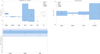 |
Fig. 5. Comparison to the B16 (left panels) and Borexino (right panel) fluxes, as in Fig. 1, but here for SSMs computed with different opacity data sets. |
4.2.1. Comparison to neutrino fluxes and P0
In Fig. 5, the OPLIB model fails at reproducing the fluxes whichever the observational set is considered. The discrepancy is maximum for Φ(B), which is 12σ lower than the B16 value. The departure is evidently worst with the Borexino value of this same flux. The comparison with Φ(CNO) also marks a clear distinction between the OPLIB SSM and the three other ones. The former is half the value measured by Borexino.
The deteriorating effect on fluxes by OPLIB were already anticipated by mean of a differential approach in Young (2018). We confirm it by a direct SSM calibration. The OPLIB decrease in the opacity of the solar radiative layers leads to a significant drop of the central temperature. To compensate and maintain the solar luminosity, the nuclear energy production by pp chain is increased, partly through an increase in Xc (see Table 3). According to the more precise data of B16, the OPLIB model overestimates production by the main pp chain. It calls for further investigation on the origin of the opacity decrease in OPLIB data for conditions corresponding to the solar radiative regions.
The effects of OP and OPAS on Xc, Zc and Tc in comparison to OPAL are small enough that they are undistinguishable from the comparisons to neutrino fluxes. As we work with the AGSS09 composition, we reach the same conclusion for the three SSMs, which is a fair agreement with the B16 data, but close to discrepancy with the Borexino set. We nevertheless observe variation of 10−20 s in P0 between the solar calibrations made with these three opacity datasets. With the seemingly attainable precision on the period spacing by Fo17 method, this indicator would be in principle useful to probe the accuracy of opacity in solar models.
The reason for this sensitivity is easy to understand from the right panel of Fig. 6, where we have N, ∇T, and the integral of N/R as a function of r (determining the value of P0). The regions responsible for the distinct values of P0 between the OPAL, OP, and OPAS SSMs are located in r/R < 0.2. There appear differences in N due to the changes induced on ∇T depending on the opacity. The period spacing of the OPLIB model presents a larger variation because ∇T is affected by a larger amplitude and on a much larger extent of the radiative region, up to r/R ∼ 0.65, very close to the base of the convective zone.
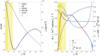 |
Fig. 6. Comparison of acoustic variables in SSMs computed with different opacity tables, as reported in the legend of the left panel. Left panel: sound speed derivative and density as a function of the radius. Right panel: N, ∇T, μ, and the integral of N/r along the radius. The meaning of the different curves in the panels are given in their respective legends. The areas shaded in yellow and light yellow respectively indicate the regions (starting from r/R = 0) in which ∼95% of Φ(B) and Φ(N) are emitted. |
4.2.2. Frequency ratios
Figure 7 reveals that OP does not improve the reproduction of the ratios in comparison to OPAL, whereas OPAS does worsen it. However, the OPLIB SSM significantly improves the fit. The effects of opacity are considerable since the seismic merit function (OPAL as reference) can be divided by a factor of more than three by OPLIB or may also be twice as large with OPAS, as shown in Table 3.
The profile of dc/dr in the left panel of Fig. 6 explains the reason behind this behaviour. While it is similar in the OPAL, OP, and OPAS models, it differs greatly over the whole radiative region in the OPLIB case. The density profiles of the four SSMs are barely affected. Therefore, the changes observed in dc/dr arise from the differences in the temperature profile and the readjustment of the other thermodynamic quantities, in particular, the pressure.
The present case illustrates the need to consider as many constraints as possible to inspect the central structure of the Sun with solar models. Some compensatory effects can indeed lead to an apparent good agreement based on the sole seismic indicators, as with the OPLIB SSM. However, a closer inspection based on comparisons with the solar neutrinos indicates a clear issue with the central physical conditions of the same model. In that context, the g-mode period spacing sensitivity on ∇T in the central layer emerges as an invaluable tool for complementing these indicators. We indeed see in Fig. 6 that the variables impacting its value vary most (between the different SSMs) in regions located between the most central ones, which are more efficiently probed with help of the neutrino fluxes (see yellow regions in the figure), and the more superfical ones (≳0.2 r/R), which the frequency ratios are more sensitive to.
4.3. Nuclear reaction rates
Here, we again adopted the AGSS09 mixture and OPAL opacities as the common ingredients (out of the reactions rates) of the SSMs presented in this section. As expected, the choice of a given set of nuclear reaction rates essentially impacts the neutrino fluxes given by the models. In first considering the three collections of rates detailed in Sect. 3, we see in Fig. 8 that the NACRE SSM is the least accordant to the observed fluxes, either from the B16 or Borexino compilations. In particular, the difference with NACRE II and SF-II is due to Φ(B): the underestimation of this flux is also the main reason for the degradation of  for this SSM in Table 4. The comparison made in Xu et al. (2013) between NACRE and NACRE II pinpoints at the origin of this difference of flux: NACRE rates are lower by a few percent, and of an almost same amount over all temperatures, for the 2H(p,γ)3He and 3He(α,γ)7Be reactions, which are both progenitors to the formation of 8B.
 |
Fig. 8. Comparisons to the B16 (left panel) and Borexino fluxes (right panel), as in Fig. 1 excepting the lower left panel not reproduced, but here for SSMs computed with different sets of nuclear reaction rates. |
We also see in Fig. 8 a clear distinction between the two SSMs with NACRE II and SF-II sets on the Borexino CNO flux, mostly due to the difference in Φ(O). From the values in Table 4, the flux predicted by the NACRE II model exceeds – by ∼16.8% – that of the SF-II model. A careful check of the models and the reaction rates reveals three reasons for this significant difference. The dominant term comes from the difference in the S-factor S(O) of the 14N(p,γ)15O reaction, which differs by ∼8% between SF-II and NACRE II. This is a consequence of the distinct methods used for the computation of the reaction rates between the two sets, the former based on the R-matrix and the latter on the potential model. This leads to differences varying from ∼10 to 12%, depending on the temperature, in the rate of this reaction between the two SSMs. We also find a difference of ∼1% in the density of the radiative layers between the two models, contributing to an increase in the flux of the NACRE II SSM. Finally, this same SSM present a larger central temperature, which also contributes to an increase for Φ(O).
The comparison with the Borexino Φ(CNO) supports its strong potential in exploring the uncertainties affecting the 14N(p,γ)15O reaction rate; here, the change of this rate in NACRE II improves and shifts closer to an agreement at 1σ a SSM with the AGSS09 mixture (see the right panel of Fig. 8). Improving the precision on this flux would be helpful not only to tighten the central solar composition, but also to explore the rates of the CNO cycle, in particular, of its bottleneck reaction.
The helioseismic constraints are less impacted by changes in the nuclear reaction rates. The ratios are barely affected in Fig. 8 and  varies ≲10%. In comparison, with a change of the composition (increase in the Ne abundance) or the opacity,
  could be divided or increased by up to a factor 2. The reason for this is given in the two previous sections: a change in these physical ingredients has more direct consequences on the central mean molecular weight or temperature, which are two key parameters of the seismic structure. Similarly, P0 between the three reference sets for nuclear rates are affected to a lower extent (7 s at most) than with other changes in the physics of the SSMs.
4.3.1. Parametric increase in pp reaction rates
The impact of nuclear processes on the computation of a SSM is not limited to the selection of a reference set for the reaction rates. Uncertainties of various orders affect the nuclear parameters of solar models. We have tried to explore part of these uncertainties by computing a new series of SSM calibrations, focusing on two aspects. First, the uncertainties themselves on nuclear reaction rates that we tested by introducing ad hoc modification of the rates in a restricted set of reactions. Next, we went further by assessing the uncertainties on the screening effects, a major process affecting the nuclear reaction rates. This is detailed in the following section (Sect. 4.3.2).
It is not the purpose of this work to explore the uncertainties affecting each of the reactions in the pp chains and CNO cycle. A recent investigation of the dependence of neutrino fluxes predicted by models on abundances, central temperatures and S-factors is presented in Villante & Serenelli (2021). Their work is based on linear pertubations of standard solar models and allows for the consideration of dependences on an extended number of nuclear reactions. Our approach is different and cannot be extended as far since we also consider the impact of evolution on predictions of solar models. We hence restricted to the proton-proton (Eq. (1)) and the 2H(p,γ)3He (hereafter d+p) reactions, for they ignite the three pp subchains. The p+p reaction rate is only accessible via numerical computations. Adelberger et al. (2011) estimate an uncertainty of about 1% affecting its determination. For the second reaction, the same authors give an uncertainty around 10%.
Given that we cannot experimentally confront the p+p computations, we exaggerated the uncertainty on it, taking into account a possible error of 5%. By this mean, we also wanted to stress the limits of observational constraints and looked at whether they would be sensible to such extreme change. So, we calibrated two additional SSMs, in the first case including an ad hoc increase by 5% of the p+p simultaneously with an increase by 10% of the d+p rate. In the second case, the two rates were decreased by 5 and 10%, respectively. In each case, we modified the two rates of the SF-II compilation, while we kept the other rates of the same compilation unaltered. The results are given in the last two columns of Table 4 and in Fig. 9 (red symbols).
 |
Fig. 9. Comparisons to the B16 (left panel) and Borexino fluxes (right panel), as in Fig. 1, excepting the lower left panel not reproduced, but now for SSMs computed with nuclear screening factors parametrically decreased or increased. |
These modifications do not alter Φ(pp) to the point of being in disagreement with the solar values of B16 or Borexino. However, since the calibration is done under the constraint of reproducing L⊙, there is a balancing effect that leads Tc to decrease when p+p and d+p rates are increased. In this SSM, as most of the production of energy comes from pp chains, p+p production in the models is slightly altered because if not, the luminosity would exceed the solar one. The associated Φ(pp) consequently remains within the error margins of the observed fluxes. However, the ratio of pp to CNO energy generation is much more affected and Φ(CNO) presents a larger discrepancy with the Borexino data. With both observational set,  actually degrades significantly. This does not support increases in the p+p and d+p reaction rates, a result that is similar to Ayukov & Baturin (2017), who explored the impact of increasing the p+p rate.
The SSM with the decreased rates sees its agreement with the B16 data degraded, mostly due to an increase in its predicted Φ(B). On the contrary, its match with the Borexino set benefits of a large improvement. We now face a model with the AGSS09 mixture closely reproducing the dominant fluxes of the pp chains as derived with Borexino data. Moreover, by factoring in an increase in Tc, the difference between the model and observed values of Φ(CNO) is reduced. In this case, testing the uncertainties of the p+p and d+p rate with the help of neutrino observations is ambiguous. Depending on the set of observed fluxes considered, we improve or worsen the reproduction of the fluxes. There again, the potential of combining neutrino with seismic constraints appears rich. Indeed, while the SSM with reduced rates present frequency ratio of poorer quality (although this is the case of all the models with AGSS09 mixture), its period spacing presents a significant drop of ∼25 s in comparison to models with no ad hoc changes. The P0 of the SSM with increased rates instead increases by a similar amount. This again reflects the sensitivity of this indicator on the profile of temperature in the central layers of the solar models.
4.3.2. Nuclear screening factors
As discussed in Sect. 3, the rates of nuclear reactions in the stellar models are boosted by the screening effect of the mean Coulomb field from the plasma. The inclusion of refined treatments of the interactions, in particular, dynamical effects is a tough task. Some attempts have shown that such effects could modify the screening factors of some reactions by a few percent (Shaviv 2007, 2010). Hence, we calibrated four additional SSMs, where we artificially multiplied the screening factors of all the reactions by identical factors of 0.90, 0.95, 1.05, and 1.10. The fluxes and P0 of these four SSMs are reported in Table 5.
Modifying the screening factors immediately impacts the central temperature of the solar models, as seen in Table 5. A decrease (resp. increase) of the screening effect means that for a fixed set of temperature, density, and composition, the number of nuclear reactions occurring is expected to decrease (resp. increase). Since the total energy that must be produced by a SSM is fixed and since the amount of energy released by each reaction is independent, a similar total number of reactions throughout the star will be necessary to ensure the SSM radiates 1 L⊙. To maintain the total number of reaction, an increase (resp. decrease) of Tc is required with a decrease (resp. increase) of screening factors. Of course some other evolutionary changes can affect the structure of the calibrated SSM, so that the ratio of pp- to CNO-produced energy can vary. But the dominant balance will remain ensured by a warming or a cooling of the core given the highly sensitive dependence of both pp and CNO nuclear energy production to temperature.
The Φ(pp) of the four SSMs with modified screening factors cannot be discriminated using the comparison to observations, as the margin errors on this flux remain too large. The Φ(Be) and Φ(B) are more sensitive to Tc and their values significantly differ between the SSMs. The increase in the screening effect reduces ϕ(B) of the two increased SSMs in such a way that their disagreement with the value of B16 grows stronger, as shown in Fig. 9. The situation is of course even worse with the Borexino data, for which Φ(Be) and Φ(B) predicted by the two SSMs clearly disagree.
The tendency is reverse for the two SSMs with decreased factors. The mild decrease of 5% restore matching between the fluxes predicted by an AGSS09 SSM and the B16 observations (see the left panel of Fig. 9). It needs a larger decrease – of 10% – for an AGSS09 SSM to then perfectly match the Borexino Φ(Be) and Φ(B). Then, it also is nearly restored to 1σ with regard to the agreement with Φ(CNO).
The comparison to helioseismic indicators reveals an opposite situation. It is an increase in the screening effect that improve the fitting of the frequency ratios by AGSS09 SSMs. We indeed observe the same behaviour as with the use of the OPLIB opacities in Sect. 4.2. A decrease in the central temperature modifies ∇T and sees a rebalancing of other thermodynamic quantities, in particular P, so that changes in dc/dr result in a better reproduction of the ratios. The same change in the central temperature considerably affects P0 of the fours SSMs with modified screening factors. Its values vary by almost 100 s between the four models, which goes well beyond the expected observational precision.
4.4. Equation of state and microscopic diffusion
The microscopic processes considered in this section include the different equations of state currently available for solar models, along with a consideration of the impact of details in the treatment of diffusion.
As expected, the choice of the equation of state has very little influence on the physical conditions at the centre of the models. Central temperature values for SSMs (AGSS09 mixture) with the equations of state Free, CEFF, OPALO5, or SAHA-S are almost identical, as shown in Tables 2 and 6. As the central compositions are almost identical between these SSMs, we do not observe any significant differences between their neutrino fluxes. And the conclusions obtained at the Sect. 4.1 for the AGSS09 and FreeEOS SSM remain valid despite the change in the equation of state. This lack of noticeable effect in the centre is not surprising because, as we mention in Sect. 3, the properties of the plasma in the core layers are in first approximation those of a perfect gas.
A slight difference appears at the level of helioseismic indicators, for which the CEFF SSM reproduces a little better the frequency ratios. The CEFF equation has originally been improved for the purpose of the solar models to better reproduce the helioseismic data, which might explain this behaviour. The same SSM also presents the largest period spacing among the different equations of state; its P0 is approximately 5 s higher than the other four SSMs, although such an increase is modest compared to the effects of other physical ingredients on this indicator.
In a final test, we included departures to perfect gas description of the plasma in the microscopic diffusion routines. Such effects were accounted for with the help of collision integrals from Paquette et al. (1986). As reported in Table 6, this treatment of the diffusion in a SSM with AGSS09 amplifies the difference with the observed neutrino datasets and the frequency ratios.
The effect of a change in the diffusion routine is of evolutionary nature. Because the solar surface abundances are used as constraints, introducing a more or less efficient settling of the elements by diffusion will require the adaptation of the initial composition of the solar calibration. It is indeed the case with the Paquette integrals, for which the SSM presents a lower initial metallicity. As a balancing effect, Tc of the model decreases to 15.50 × 10⁶ K, which disfavours the reproduction of neutrino observations.
5. Discussion: Comparisons with the literature
Certain ingredients of the solar models, such as the chemical mixture, play a dominant role in the theoretical fluxes and orient the interpretation of solar neutrino data. Another aspect to consider is how dependent it is on the stellar evolution code itself. To address this, we can compare our SSM flux values to models with the most equivalent physics from other works in the literature (e.g. Boothroyd & Sackmann 2003 for a previous generation of solar models).
To this aim, we first compared our results to SSMs computed with the GARSTEC code (Weiss & Schlattl 2008) and presented in Serenelli et al. (2009). We focused on the two SSMs they made with the GS98 and AGSS09 mixture, which we refer to as SSM-GS98-S09 and SSM-AGSS09ph-S09. The properties of these models are summarised in Table 7, while those of our two SSMs with the corresponding mixtures were given in Table 2. Their nuclear network is based on references presented in Bahcall & Pinsonneault (1995), but includes LUNA updates, while they use OPAL opacities and equation of state. We focus on Φ(Be) and Φ(B) because they are more sensitive to details of the core structure, in particular the temperature. These fluxes in our GS98 SSM are larger by 1%, while they are lower by ∼2 and 4% in the AGSS09 case. The Φ(CNO) differs more considerably, as our SSMs estimate them larger by 10−15%. To the contrary, the chemical compositions at the centre are very similar; the metallicities are close by less than 1% and X are < 1% in the AGSS09 case and 1.5% in the GS98 one. These differences in Φ(Be) and Φ(B) are likely due to a mix of differences in Tc and nuclear rates. Those affecting Φ(CNO) are more likely related to differences in the nuclear rates.
Central conditions and neutrino fluxes from a selection of standard solar models in the literature (see main text for the references).
In Vinyoles et al. (2017), an updated GARSTEC GS98 SSM is presented, which we refer to as SSM-GS98-V17 (see Table 7). The SSM-GS98-V17 model shares the same reference for the nuclear reaction rates than us, SF-II, though it is built with OP instead of OPAL in our case. The Φ(Be) and Φ(B) of our GS98 SSM are now larger by 3.7% and 8.4%. The composition presents similar differences than in the above comparison, with Xc and Zc, respectively, 1.4% and 1% higher in our model. The update in Vinyoles et al. (2017) has actually profoundly reduced the value that was previously found for Φ(B). The reason for this effect is not clear since the main element of the update was the revision of the nuclear reaction rates, which are now the same as the GS98 SSM we calibrated. Since this flux is extremely sensitive to the core temperature, the difference in Tc appears as a good candidate to explain the important discrepancy in Φ(B). However, in referring to Sect. 4.2, the effect on Tc regarding a change of opacity from OP to OPAL is not sufficient to explain such a difference in Φ(B). It suggests we are facing a larger difference in Tc from another origin between our model and the SSM-GS98-V17 one. It is only more detailed comparisons of the structures of each model that could help explain the origin of this discrepancy.
Zhang et al. (2019) computed with the YNEV code (Zhang 2015) SSMs with GS98 and AGSS09 mixtures (respectively the SSM-GS98-Zh19 and SSM-AGSS09-Zh19 in Table 7), including OPAL opacities, and nuclear rates from the SF-II project, a set of physics that allows for more direct comparisons with our work. For instance, we find values of Φ(B) larger by 10.6% 5.8% and Φ(CNO) larger by 9.2 and 5.3% respectively in the GS98 and AGSS09 cases. Thanks to the central temperatures of their models, given in Zhang et al. (2019), we can estimate the difference in Tc with our SSMs to be 0.38% and 0.14%, respectively, in the GS98 and AGSS09 case. They are of the same order as the differences in Tc resulting between our SSMs when we vary the chemical mixtures.
The differences are not surprising since stellar codes will intrinsically differ: internal error of the models, differences in the numerical schemes, but also differences in minor physical aspects. For instance, we noted that the reference value adopted for L⊙ is lower in our models by 0.36% than that used in Vinyoles et al. (2017) and Zhang et al. (2019). Therefore, we have to bear in mind that even with similar physics, fluxes predicted by different stellar evolution codes can differ by the same order as the differences found between sets of observed neutrinos (see B16 vs Borexino) or between models with different mixtures. We should be cautious that it can hence radically change our interpretation of the neutrino fluxes. It calls for more detailed comparisons of stellar codes to identify and quantify the distinct sources that cause them to differ.
6. Conclusions
The recent announcement by Fossat et al. (2017) regarding the detection of a series of solar g modes and their rotational splittings has promised new constraints on the central layers of the Sun (see also Eggenberger et al. 2019, on exploring magnetic angular momentum transport processes). The reliability of the detection is seriously questioned by independent attempts to recover it (Schunker et al. 2018; Scherrer & Gough 2019; Appourchaux & Corbard 2019). But, the constant spacing predicted by the asymptotic theory between the periods of g modes, P0, offers, in principle, a valuable complement to the solar neutrino fluxes. Despite the fragile status of the detection, the method detailed in Fossat et al. (2017) and Fossat & Schmider (2018), shows that the determination of P0 is reachable to a high degree of precision. Adopting this precision, we can anticipate the constraint provided by P0 on the standard solar models.
We have thus compared the theoretical P0 values predicted by a set of standard solar models for which we have varied the main ingredients of internal physics: chemical mixture, opacity, nuclear reactions, equation of state. In complement to early results based on seismic models of the Sun by Buldgen et al. (2020), we confirm that the reported g-mode period spacing is incompatible with the values predicted by standard solar models. In comparison to that of Fossat et al. (2017), P0 = 2041 ± 1 s, all of the models predict a value to be larger by 100 to 150 s. Nevertheless, with the same level of precision, we find that it is possible to distinguish solar models calibrated with different chemical composition, opacity, and to a lesser extent and with some degeneracy, screening factors and nuclear reaction rates. It is the sensitivity of P0 to the mean molecular weight in the central layers that affords to discriminate different chemical mixtures and compositions. For instance, P0 changes by ∼20 s between low- and high-metallicity models. The sensitivity of P0 to the temperature gradient also enables it to distinguish changes in the opacity. Between usual reference opacity sets, the value of P0 typically varies by ∼10 s. In complement with the frequency ratios of the solar pressure modes, which are also sensitive to the mean molecular weight (Chaplin et al. 2007), the g-mode period spacing would bring helioseismology to an unprecedented level of precision to constrain the deep layers of the Sun. We estimate that the value P0 in the Sun should most likely lie between 2150 and 2190 s.
We also compared the neutrino fluxes predicted by our models to those reported in the meta-analysis by Bergström et al. (2016), and the most recent results of the Borexino Collaboration. Although the values of Bergström et al. (2016) and Borexino are in agreement, the difference in the flux Φ(B) is significant and can lead to a different interpretation of the comparison with models. The low-metallicity solar models better reproduce the B16 data while high-metallicity are preferred for the Borexino dataset. The Φ(CNO), which is for the first time entirely determined in Borexino, strengthens this preference. An improvement in the precision (presently at the level of ∼40%) on this flux will clearly help to refine the question of abundances, in particular of metals, in the solar radiative regions. When also taking into account the helioseismic frequency ratios, the high-metallicity models clearly continue to be in better agreement with solar data (confirming the results based on ratios by Basu et al. 2007).
The comparison to neutrino fluxes from a standard model with the recent OPLIB opacities has shown an important discrepancy. Despite the fact that the OPLIB solar model better reproduces the frequency ratios, it is clearly incompatible with observed fluxes, which it underestimates by a large amount.
We looked in detail at the potential impact of a revision of nuclear screening factors. These, in the framework of the so-called low-interaction regime, are currently described in most stellar models without inclusion of finer effects, such as those related to particle movements (e.g. Mussack & Däppen 2011). These effects are difficult to compute and incorporate in stellar models. Nevertheless, first estimates show that factors could differ up to a few percent (Shaviv 2004, 2007). We have tested ad hoc decreases and increases of the factors. We find that a decrease by 5−10% would lead the low-metallicity models to match neutrino observations, but without improving their fit of the frequency ratios. This is also a consequence of the regions which the different indicators are sensitive to; the neutrino fluxes probe the nuclear core, the period spacing its close vicinity, where only a superficial number (< 5%) of nuclear reactions take place and, finally, the frequency ratios more superficial radiative regions.
This last point highlights the possibility of testing multiple aspects of solar physics with the consideration of the full observational data at our disposal. For instance, a constraint such as the present solar surface lithium abundance or the reproduction of all the helioseismic inverted acoustic variables are met by neither high-metallicity nor with low-metallicity solar models (e.g. Buldgen et al. 2020). The solar issue remains open and likely calls for improvements to standard or non-standard stellar physics, which we can test in detail using an advanced set of observational indicators. In particular, the possibility to have constraints from gravity modes would help us further refine our understanding of the solar core properties. Here, we show that a period spacing value constrained within one or two seconds would prove very selective with regard to the properties of solar models. In that respect, the quest for solar gravity modes still remains of paramount importance for studies of the structure and rotation of the solar core.
See details and references in the B16 paper.
In Vinyoles et al. (2017), they actually use the AGSS09 mixture but with meteoritic abundances preferred for refractory elements.
I.e. non nuclear-processed material.
Acknowledgments
We thank N. Grevesse for helpful comments. S.J.A.J.S., P.E. and G.M. have received funding from the European Research Council (ERC) under the European Union’s Horizon 2020 research and innovation programme (grant agreement No 833925, project STAREX). G.B. acknowledges fundings from the SNF AMBIZIONE grant No. 185805 (Seismic inversions and modelling of transport processes in stars) and support by the ISSI team “Probing the core of the Sun and the stars” (ID 423).
References
- Abe, K., Haga, Y., Hayato, Y., et al. 2016, Phys. Rev. D, 94, 052010 [NASA ADS] [CrossRef] [Google Scholar]
- Adelberger, E. G., García, A., Robertson, R. G. H., et al. 2011, Rev. Mod. Phys., 83, 195 [NASA ADS] [CrossRef] [Google Scholar]
- Aharmim, B., Ahmed, S. N., Anthony, A. E., et al. 2013, Phys. Rev. C, 88, 025501 [NASA ADS] [CrossRef] [Google Scholar]
- Amarsi, A. M., Barklem, P. S., Collet, R., Grevesse, N., & Asplund, M. 2019, A&A, 624, A111 [NASA ADS] [CrossRef] [EDP Sciences] [Google Scholar]
- Amarsi, A. M., Grevesse, N., Grumer, J., et al. 2020, A&A, 636, A120 [CrossRef] [EDP Sciences] [Google Scholar]
- Angulo, C., Arnould, M., Rayet, M., et al. 1999, Nucl. Phys. A, 656, 3 [Google Scholar]
- Antia, H. M., & Basu, S. 2005, ApJ, 620, L129 [NASA ADS] [CrossRef] [Google Scholar]
- Antia, H. M., & Chitre, S. M. 1995, ApJ, 442, 434 [CrossRef] [Google Scholar]
- Antia, H. M., & Chitre, S. M. 1998, A&A, 339, 239 [NASA ADS] [Google Scholar]
- Antia, H. M., & Chitre, S. M. 2002, A&A, 393, L95 [CrossRef] [EDP Sciences] [Google Scholar]
- Appourchaux, T., & Corbard, T. 2019, A&A, 624, A106 [NASA ADS] [CrossRef] [EDP Sciences] [Google Scholar]
- Appourchaux, T., & Pallé, P. L. 2013, in Fifty Years of Seismology of the Sun and Stars, eds. K. Jain, S. C. Tripathy, F. Hill, J. W. Leibacher, & A. A. Pevtsov, ASP Conf. Ser., 478, 125 [NASA ADS] [Google Scholar]
- Appourchaux, T., Belkacem, K., Broomhall, A. M., et al. 2010, A&ARv, 18, 197 [Google Scholar]
- Asplund, M., Grevesse, N., & Sauval, A. J. 2005, in Cosmic Abundances as Records of Stellar Evolution and Nucleosynthesis, eds. T. G. Barnes, III, & F. N. Bash, ASP Conf. Ser., 336, 25 [Google Scholar]
- Asplund, M., Grevesse, N., Sauval, A. J., & Scott, P. 2009, ARA&A, 47, 481 [NASA ADS] [CrossRef] [Google Scholar]
- Ayukov, S. V., & Baturin, V. A. 2017, Astron. Rep., 61, 901 [CrossRef] [Google Scholar]
- Badnell, N. R., Bautista, M. A., Butler, K., et al. 2005, MNRAS, 360, 458 [Google Scholar]
- Bahcall, J. N. 2002, Phys. Rev. C, 65, 025801 [NASA ADS] [CrossRef] [Google Scholar]
- Bahcall, J. N., & Pinsonneault, M. H. 1995, Rev. Mod. Phys., 67, 781 [NASA ADS] [CrossRef] [Google Scholar]
- Bahcall, J. N., & Ulrich, R. K. 1988, Rev. Mod. Phys., 60, 297 [NASA ADS] [CrossRef] [Google Scholar]
- Bahcall, J. N., Huebner, W. F., Lubow, S. H., Parker, P. D., & Ulrich, R. K. 1982, Rev. Mod. Phys., 54, 767 [NASA ADS] [CrossRef] [Google Scholar]
- Bahcall, J. N., Krastev, P. I., & Smirnov, A. Y. 1998, Phys. Rev. D, 58, 096016 [NASA ADS] [CrossRef] [Google Scholar]
- Bahcall, J. N., Basu, S., Pinsonneault, M., & Serenelli, A. M. 2005, ApJ, 618, 1049 [NASA ADS] [CrossRef] [Google Scholar]
- Bahcall, J. N., Serenelli, A. M., & Basu, S. 2006, ApJS, 165, 400 [NASA ADS] [CrossRef] [Google Scholar]
- Bailey, J., Nagayama, T., Loisel, G., et al. 2014, Nature, 517, 56 [NASA ADS] [CrossRef] [PubMed] [Google Scholar]
- Basu, S. 2016, Liv. Rev. Sol. Phys., 13, 2 [Google Scholar]
- Basu, S., & Antia, H. M. 1995, MNRAS, 276, 1402 [NASA ADS] [Google Scholar]
- Basu, S., & Antia, H. M. 2008, Phys. Rep., 457, 217 [Google Scholar]
- Basu, S., Chaplin, W. J., Elsworth, Y., et al. 2007, ApJ, 655, 660 [NASA ADS] [CrossRef] [Google Scholar]
- Baturin, V. A., Ayukov, S. V., Gryaznov, V. K., et al. 2013, in Progress in Physics of the Sun and Stars: A New Era in Helio- and Asteroseismology, eds. H. Shibahashi, & A. E. Lynas-Gray, ASP Conf. Ser., 479, 11 [Google Scholar]
- Bellini, G., Benziger, J., Bick, D., et al. 2012, Phys. Rev. Lett., 108, 051302 [CrossRef] [PubMed] [Google Scholar]
- Bergström, J., Gonzalez-Garcia, M. C., Maltoni, M., et al. 2016, J. High Energy Phys., 2016, 132 [CrossRef] [Google Scholar]
- Berthomieu, G., & Provost, J. 1991, Sol. Phys., 133, 127 [NASA ADS] [CrossRef] [Google Scholar]
- Blancard, C., Cossé, P., & Faussurier, G. 2012, ApJ, 745, 10 [NASA ADS] [CrossRef] [Google Scholar]
- Boothroyd, A. I., & Sackmann, I. J. 2003, ApJ, 583, 1004 [NASA ADS] [CrossRef] [Google Scholar]
- Borexino Collaboration (Agostini, M., et al.) 2018, Nature, 562, 505 [NASA ADS] [CrossRef] [Google Scholar]
- Borexino Collaboration (Agostini, M., et al.) 2020, Nature, 587, 577 [CrossRef] [Google Scholar]
- Brown, T. M., Christensen-Dalsgaard, J., Dziembowski, W. A., et al. 1989, ApJ, 343, 526 [NASA ADS] [CrossRef] [Google Scholar]
- Buldgen, G., Salmon, S. J. A. J., Noels, A., et al. 2017, MNRAS, 472, 751 [CrossRef] [Google Scholar]
- Buldgen, G., Salmon, S., & Noels, A. 2019, Front. Astron. Space Sci., 6, 42 [CrossRef] [Google Scholar]
- Buldgen, G., Eggenberger, P., Baturin, V. A., et al. 2020, A&A, 642, A36 [EDP Sciences] [Google Scholar]
- Caffau, E., Ludwig, H.-G., Steffen, M., Freytag, B., & Bonifacio, P. 2011, Sol. Phys., 268, 255 [Google Scholar]
- Cassisi, S., Potekhin, A. Y., Pietrinferni, A., Catelan, M., & Salaris, M. 2007, ApJ, 661, 1094 [NASA ADS] [CrossRef] [Google Scholar]
- Chaplin, W. J., Serenelli, A. M., Basu, S., et al. 2007, ApJ, 670, 872 [NASA ADS] [CrossRef] [Google Scholar]
- Christensen-Dalsgaard, J. 2002, Rev. Mod. Phys., 74, 1073 [NASA ADS] [CrossRef] [Google Scholar]
- Christensen-Dalsgaard, J. 2021, Liv. Rev. Sol. Phys., 18, 2 [CrossRef] [Google Scholar]
- Christensen-Dalsgaard, J., & Daeppen, W. 1992, A&ARv, 4, 267 [NASA ADS] [CrossRef] [Google Scholar]
- Christensen-Dalsgaard, J., Duvall, T. L., Jr., Gough, D. O., Harvey, J. W., & Rhodes, E. J., Jr. 1985, Nature, 315, 378 [NASA ADS] [CrossRef] [Google Scholar]
- Christensen-Dalsgaard, J., Gough, D. O., & Thompson, M. J. 1991, ApJ, 378, 413 [NASA ADS] [CrossRef] [Google Scholar]
- Christensen-Dalsgaard, J., Proffitt, C. R., & Thompson, M. J. 1993, ApJ, 403, L75 [NASA ADS] [CrossRef] [Google Scholar]
- Colgan, J., Kilcrease, D. P., Magee, N. H., et al. 2016, ApJ, 817, 116 [Google Scholar]
- Cox, J. P., & Giuli, R. T. 1968, Principles of Stellar Structure (New York: Gordon and Breach) [Google Scholar]
- Davis, R., Harmer, D. S., & Hoffman, K. C. 1968, Phys. Rev. Lett., 20, 1205 [CrossRef] [Google Scholar]
- Davies, G. R., Broomhall, A. M., Chaplin, W. J., Elsworth, Y., & Hale, S. J. 2014, MNRAS, 439, 2025 [Google Scholar]
- degl’Innocenti, S., Fiorentini, G., & Ricci, B. 1998, Phys. Lett. B, 416, 365 [CrossRef] [Google Scholar]
- Delache, P., & Scherrer, P. H. 1983, Nature, 306, 651 [Google Scholar]
- Dzitko, H., Turck-Chieze, S., Delbourgo-Salvador, P., & Lagrange, C. 1995, ApJ, 447, 428 [CrossRef] [Google Scholar]
- Eggenberger, P., Buldgen, G., & Salmon, S. J. A. J. 2019, A&A, 626, L1 [NASA ADS] [CrossRef] [EDP Sciences] [Google Scholar]
- Eggleton, P. P., Faulkner, J., & Flannery, B. P. 1973, A&A, 23, 325 [NASA ADS] [Google Scholar]
- Elliott, J. R., & Kosovichev, A. G. 1998, ApJ, 500, L199 [NASA ADS] [CrossRef] [Google Scholar]
- Ellis, A. N. 1986, in Seismology of the Sun and the Distant Stars, ed. D. O. Gough, NATO Advanced Study Institute (ASI) Series C, 169, 173 [CrossRef] [Google Scholar]
- Ferguson, J. W., Alexander, D. R., Allard, F., et al. 2005, ApJ, 623, 585 [Google Scholar]
- Formicola, A., Imbriani, G., Costantini, H., et al. 2004, Phys. Lett. B, 591, 61 [Google Scholar]
- Fossat, E., & Schmider, F. X. 2018, A&A, 612, L1 [NASA ADS] [CrossRef] [EDP Sciences] [Google Scholar]
- Fossat, E., Boumier, P., Corbard, T., et al. 2017, A&A, 604, A40 [NASA ADS] [CrossRef] [EDP Sciences] [Google Scholar]
- Fröhlich, C., & Lean, J. 1998, Geophys. Res. Lett., 25, 4377 [NASA ADS] [CrossRef] [Google Scholar]
- Fukuda, Y., Hayakawa, T., Ichihara, E., et al. 1999, Phys. Rev. Lett., 82, 1810 [CrossRef] [Google Scholar]
- Gabriel, A. H., Grec, G., Charra, J., et al. 1995, Sol. Phys., 162, 61 [NASA ADS] [CrossRef] [Google Scholar]
- García, R. A., Turck-Chièze, S., Jiménez-Reyes, S. J., et al. 2007, Science, 316, 1591 [Google Scholar]
- Gonzalez, G. 2006, MNRAS, 370, L90 [CrossRef] [Google Scholar]
- Gough, D. 2003, Astrophys. Space Sci., 284, 165 [NASA ADS] [CrossRef] [Google Scholar]
- Gough, D. O. 2019, MNRAS, 485, L114 [CrossRef] [Google Scholar]
- Grevesse, N., & Noels, A. 1993, in Origin and Evolution of the Elements, eds. N. Prantzos, E. Vangioni-Flam, & M. Casse, 15 [Google Scholar]
- Grevesse, N., & Sauval, A. J. 1998, Space Sci. Rev., 85, 161 [Google Scholar]
- Grevesse, N., Asplund, M., Sauval, J., & Scott, P. 2013, Eur. Phys. J. Web Conf., 43, 01004 [CrossRef] [Google Scholar]
- Grevesse, N., Scott, P., Asplund, M., & Sauval, A. J. 2015, A&A, 573, A27 [NASA ADS] [CrossRef] [EDP Sciences] [Google Scholar]
- Gruzinov, A. V., & Bahcall, J. N. 1998, ApJ, 504, 996 [NASA ADS] [CrossRef] [Google Scholar]
- Gryaznov, V. K., Ayukov, S. V., Baturin, V. A., et al. 2004, in Equation-of-State and Phase-Transition in Models of Ordinary Astrophysical Matter, eds. V. Celebonovic, D. Gough, & W. Däppen, AIP Conf. Ser., 731, 147 [NASA ADS] [CrossRef] [Google Scholar]
- Guzik, J. A., & Mussack, K. 2010, ApJ, 713, 1108 [NASA ADS] [CrossRef] [Google Scholar]
- Guzik, J. A., Watson, L. S., & Cox, A. N. 2006, Mem. Soc. Astron. It., 77, 389 [NASA ADS] [Google Scholar]
- Hale, S. J., Howe, R., Chaplin, W. J., Davies, G. R., & Elsworth, Y. P. 2016, Sol. Phys., 291, 1 [CrossRef] [Google Scholar]
- Haxton, W., Hamish Robertson, R., & Serenelli, A. M. 2013, ARA&A, 51, 21 [NASA ADS] [CrossRef] [Google Scholar]
- Iglesias, C. A. 2015, High Energy Density Phys., 15, 4 [CrossRef] [Google Scholar]
- Iglesias, C. A., & Rogers, F. J. 1996, ApJ, 464, 943 [NASA ADS] [CrossRef] [Google Scholar]
- Imbriani, G., Costantini, H., Formicola, A., et al. 2005, Eur. Phys. J. A, 25, 455 [NASA ADS] [CrossRef] [EDP Sciences] [Google Scholar]
- Irwin, A. W. 2012, Astrophysics Source Code Library [record ascl:1211.002] [Google Scholar]
- Kosovichev, A. G. 1988, Sov. Astron. Lett., 14, 145 [NASA ADS] [Google Scholar]
- Kosovichev, A. G. 2011, in Advances in Global and Local Helioseismology: An Introductory Review, eds. J. P. Rozelot, & C. Neiner, 832, 3 [Google Scholar]
- Kosovichev, A. G., & Fedorova, A. V. 1991, Sov. Astron., 35, 507 [NASA ADS] [Google Scholar]
- Landi, E., & Testa, P. 2015, ApJ, 800, 110 [NASA ADS] [CrossRef] [Google Scholar]
- Le Pennec, M., Turck-Chièze, S., Salmon, S., et al. 2015, ApJ, 813, L42 [Google Scholar]
- Lin, C.-H., Antia, H. M., & Basu, S. 2007, ApJ, 668, 603 [Google Scholar]
- Mao, D., Mussack, K., & Däppen, W. 2009, ApJ, 701, 1204 [Google Scholar]
- Marta, M., Formicola, A., Gyürky, G., et al. 2008, Phys. Rev. C, 78, 022802 [Google Scholar]
- Marta, M., Formicola, A., Bemmerer, D., et al. 2011, Phys. Rev. C, 83, 045804 [Google Scholar]
- Mondet, G., Blancard, C., Cossé, P., & Faussurier, G. 2015, ApJS, 220, 2 [Google Scholar]
- Montalbán, J., Miglio, A., Noels, A., Grevesse, N., & di Mauro, M. P. 2004, in SOHO 14 Helio- and Asteroseismology: Towards a Golden Future, ed. D. Danesy, ESA SP, 559, 574 [Google Scholar]
- Mussack, K., & Däppen, W. 2011, ApJ, 729, 96 [Google Scholar]
- Nagayama, T., Bailey, J. E., Loisel, G. P., et al. 2019, Phys. Rev. Lett., 122, 235001 [Google Scholar]
- Nahar, S. N., & Pradhan, A. K. 2016, Phys. Rev. Lett., 116, 235003 [Google Scholar]
- Pain, J.-C., & Gilleron, F. 2015, High Energy Density Phys., 15, 30 [Google Scholar]
- Paquette, C., Pelletier, C., Fontaine, G., & Michaud, G. 1986, ApJS, 61, 177 [NASA ADS] [CrossRef] [Google Scholar]
- Provost, J., & Berthomieu, G. 1986, A&A, 165, 218 [NASA ADS] [Google Scholar]
- Ricci, B., Berezinsky, V., & degl’Innocenti, S., Dziembowski, W. A., & Fiorentini, G., 1997, Phys. Lett. B, 407, 155 [Google Scholar]
- Rogers, F. J., & Nayfonov, A. 2002, ApJ, 576, 1064 [Google Scholar]
- Roxburgh, I. W., & Vorontsov, S. V. 2003, A&A, 411, 215 [NASA ADS] [CrossRef] [EDP Sciences] [Google Scholar]
- Salpeter, E. E. 1954, Aust. J. Phys., 7, 373 [Google Scholar]
- Scherrer, P. H., & Gough, D. O. 2019, ApJ, 877, 42 [Google Scholar]
- Schou, J., Antia, H. M., Basu, S., et al. 1998, ApJ, 505, 390 [Google Scholar]
- Schunker, H., Schou, J., Gaulme, P., & Gizon, L. 2018, Sol. Phys., 293, 95 [Google Scholar]
- Scott, P., Asplund, M., Grevesse, N., Bergemann, M., & Sauval, A. J. 2015, A&A, 573, A26 [NASA ADS] [CrossRef] [EDP Sciences] [Google Scholar]
- Scuflaire, R., Théado, S., Montalbán, J., et al. 2008a, Ap&SS, 316, 83 [Google Scholar]
- Scuflaire, R., Montalbán, J., Théado, S., et al. 2008b, Ap&SS, 316, 149 [Google Scholar]
- Seaton, M. J., & Badnell, N. R. 2004, MNRAS, 354, 457 [Google Scholar]
- Serenelli, A. 2016, Eur. Phys. J. A, 52, 78 [NASA ADS] [CrossRef] [EDP Sciences] [Google Scholar]
- Serenelli, A. M., Basu, S., Ferguson, J. W., & Asplund, M. 2009, ApJ, 705, L123 [Google Scholar]
- Serenelli, A., Peña-Garay, C., & Haxton, W. C. 2013, Phys. Rev. D, 87, 043001 [Google Scholar]
- Severnyi, A. B., Kotov, V. A., & Tsap, T. T. 1976, Nature, 259, 87 [Google Scholar]
- Shaviv, G. 2004, A&A, 418, 801 [EDP Sciences] [Google Scholar]
- Shaviv, G. 2007, in Tours Symposium on Nuclear Physics VI, eds. M. Arnould, M. Lewitowicz, H. Emling, et al., AIP Conf. Ser., 891, 315 [Google Scholar]
- Shaviv, G. 2010, Mem. Soc. Astron. It., 81, 77 [Google Scholar]
- Shaviv, N. J., & Shaviv, G. 2001, ApJ, 558, 925 [Google Scholar]
- Song, N., Gonzalez-Garcia, M. C., Villante, F. L., Vinyoles, N., & Serenelli, A. 2018, MNRAS, 477, 1397 [Google Scholar]
- Stonehill, L. C., Formaggio, J. A., & Robertson, R. G. H. 2004, Phys. Rev. C, 69, 015801 [Google Scholar]
- Thoul, A. A., Bahcall, J. N., & Loeb, A. 1994, ApJ, 421, 828 [NASA ADS] [CrossRef] [Google Scholar]
- Turck-Chièze, S., & Couvidat, S. 2011, Rep. Progr. Phys., 74, 086901 [Google Scholar]
- Turck-Chieze, S., & Lopes, I. 1993, ApJ, 408, 347 [Google Scholar]
- Turck-Chièze, S., Couvidat, S., Piau, L., et al. 2004, Phys. Rev. Lett., 93, 211102 [Google Scholar]
- Villante, F. L., & Serenelli, A. 2021, Front. Astron. Space Sci., 7, 112 [Google Scholar]
- Vinyoles, N., Serenelli, A. M., Villante, F. L., et al. 2017, ApJ, 835, 202 [NASA ADS] [CrossRef] [Google Scholar]
- Vorontsov, S. V., Baturin, V. A., & Pamiatnykh, A. A. 1991, Nature, 349, 49 [Google Scholar]
- Vorontsov, S. V., Baturin, V. A., Ayukov, S. V., & Gryaznov, V. K. 2013, MNRAS, 430, 1636 [Google Scholar]
- Watanabe, S., & Shibahashi, H. 2001, PASJ, 53, 565 [Google Scholar]
- Weiss, A., & Schlattl, H. 2008, Ap&SS, 316, 99 [Google Scholar]
- Wood, S. R., Mussack, K., & Guzik, J. A. 2018, Sol. Phys., 293, 111 [Google Scholar]
- Xu, Y., Takahashi, K., Goriely, S., et al. 2013, Nucl. Phys. A, 918, 61 [NASA ADS] [CrossRef] [Google Scholar]
- Young, P. R. 2018, ApJ, 855, 15 [NASA ADS] [CrossRef] [EDP Sciences] [Google Scholar]
- Zhang, Q.-S. 2015, Res. Astron. Astrophys., 15, 549 [Google Scholar]
- Zhang, Q.-S., Li, Y., & Christensen-Dalsgaard, J. 2019, ApJ, 881, 103 [CrossRef] [Google Scholar]
All Tables
Solar neutrino fluxes at 1 AU from the combined analysis of B16 and from the Borexino Collaboration (2018, 2020).
Stellar parameters of the SSMs calibrated with different solar chemical mixtures.
Central conditions and neutrino fluxes from a selection of standard solar models in the literature (see main text for the references).
All Figures
|
Fig. 1. Neutrino fluxes predicted by the standard solar models (see Sect. 3) with different chemical mixtures. The comparison to the observational fluxes derived by B16 is shown in the left panels, and to the Borexino Collaboration in the right panel. Left upper panel: two boxes are inserted to present a zoom on the Φ(pp) and P0 comparisons. In the panel at the bottom, the comparison is restricted to Φ(pp), Φ(Be) and Φ(B) from the B16 set only for the sake of clarity. The 1σ intervals on the observations are shaded in blue in the three panels. The 3σ range is shaded in light blue in the bottom panel. |
| In the text | |
|
Fig. 2. Equilibrium abundances (dashed lines) of the 8B nuclides and the cumulative neutrino flux from their disintegration, ϕ8B (solid lines), along the radial coordinate r. They are presented as a function of the temperature, for three SSMs with different chemical mixtures, as given in the legend. Abundances are in mole per gram, and the flux, as usual, is computed for an observer at 1 AU. |
| In the text | |
|
Fig. 3. Equilibrium abundances of the 12C and 14N nuclides (dashed and dotted lines) and the cumulative neutrino fluxes of the 13N and 15O disintegrations, ϕ13N and ϕ15O (solid and dot-dashed lines). They are drawn as a function of the temperature, for three SSMs with different chemical mixtures, as given in the legend. |
| In the text | |
|
Fig. 4. Comparison of solar low-degree p-mode frequency ratios r02 and r13 to those of the SSMs with different chemical mixtures. The adopted chemical mixtures are indicated in the legend. |
| In the text | |
|
Fig. 5. Comparison to the B16 (left panels) and Borexino (right panel) fluxes, as in Fig. 1, but here for SSMs computed with different opacity data sets. |
| In the text | |
|
Fig. 6. Comparison of acoustic variables in SSMs computed with different opacity tables, as reported in the legend of the left panel. Left panel: sound speed derivative and density as a function of the radius. Right panel: N, ∇T, μ, and the integral of N/r along the radius. The meaning of the different curves in the panels are given in their respective legends. The areas shaded in yellow and light yellow respectively indicate the regions (starting from r/R = 0) in which ∼95% of Φ(B) and Φ(N) are emitted. |
| In the text | |
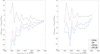 |
Fig. 7. Same as in Fig. 4 but for different adopted opacity references, as indicated in the legend. |
| In the text | |
|
Fig. 8. Comparisons to the B16 (left panel) and Borexino fluxes (right panel), as in Fig. 1 excepting the lower left panel not reproduced, but here for SSMs computed with different sets of nuclear reaction rates. |
| In the text | |
|
Fig. 9. Comparisons to the B16 (left panel) and Borexino fluxes (right panel), as in Fig. 1, excepting the lower left panel not reproduced, but now for SSMs computed with nuclear screening factors parametrically decreased or increased. |
| In the text | |
Current usage metrics show cumulative count of Article Views (full-text article views including HTML views, PDF and ePub downloads, according to the available data) and Abstracts Views on Vision4Press platform.
Data correspond to usage on the plateform after 2015. The current usage metrics is available 48-96 hours after online publication and is updated daily on week days.
Initial download of the metrics may take a while.