| Issue |
A&A
Volume 651, July 2021
|
|
|---|---|---|
| Article Number | A5 | |
| Number of page(s) | 11 | |
| Section | Astronomical instrumentation | |
| DOI | https://doi.org/10.1051/0004-6361/202140340 | |
| Published online | 06 July 2021 | |
High precision measurements of interstellar dispersion measure with the upgraded GMRT⋆
1
Fakultät für Physik, Universität Bielefeld, Postfach 100131, 33501 Bielefeld, Germany
e-mail: This email address is being protected from spambots. You need JavaScript enabled to view it.
2
Arecibo Observatory, University of Central Florida, Arecibo, PR 00612, USA
3
National Centre for Radio Astrophysics, Tata Institute of Fundamental Research, Ganeshkhind, Pune, 411007 Maharashtra, India
4
Department of Physics, Indian Institute of Technology Hyderabad, Kandi, Telangana 502285, India
5
The Institute of Mathematical Sciences, CIT Campus, Tharamani, Chennai, 600113 Tamil Nadu, India
6
Homi Bhabha National Institute, Training School Complex, Anushakti Nagar, Mumbai, 400094 Maharashtra, India
7
Department of Physics, BITS Pilani Hyderabad Campus, Hyderabad, 500078 Telangana, India
8
Department of Astronomy and Astrophysics, Tata Institute of Fundamental Research, Dr. Homi Bhabha Road, Mumbai, 400005 Maharashtra, India
9
Indian Institute of Science Education and Research Thiruvananthapuram, Vithura, Kerala 695551, India
10
Jodrell Bank Centre for Astrophysics, University of Manchester, Oxford Road, Manchester M13 9PL, UK
11
ASTRON, the Netherlands Institute for Radio Astronomy, Postbus 2, 7990 AA Dwingeloo, The Netherlands
12
Department of Physics, Indian Institute of Technology Delhi, Hauz Khas, New Delhi 110016, India
13
Cahill Center for Astrophysics, California Institute of Technology, 1200 E. California Blvd., Pasadena, CA 91125, USA
14
University of Oxford, Sub-Department of Astrophysics, Denys Wilkinson Building, Keble Road, Oxford OX1 3RH, UK
15
Department of Physics, Indian Institute of Technology Roorkee, Roorkee, 247667 Uttarakhand, India
16
Raman Research Institute, Bengaluru, 560080 Karnataka, India
Received:
13
January
2021
Accepted:
26
May
2021
Abstract
Context. Pulsar radio emission undergoes dispersion due to the presence of free electrons in the interstellar medium (ISM). The dispersive delay in the arrival time of the pulsar signal changes over time due to the varying ISM electron column density along the line of sight. Accurately correcting for this delay is crucial for the detection of nanohertz gravitational waves using pulsar timing arrays.
Aims. We aim to demonstrate the precision in the measurement of the dispersion delay achieved by combining 400−500 MHz (BAND3) wide-band data with those at 1360−1460 MHz (BAND5) observed using the upgraded GMRT, employing two different template alignment methods.
Methods. To estimate the high precision dispersion measure (DM), we measure high precision times-of-arrival (ToAs) of pulses using carefully generated templates and the currently available pulsar timing techniques. We use two different methods for aligning the templates across frequency to obtain ToAs over multiple sub-bands and therefrom measure the DMs. We study the effects of these two different methods on the measured DM values in detail.
Results. We present in-band and inter-band DM estimates of four pulsars over the timescale of a year using two different template alignment methods. The DMs obtained using both these methods show only subtle differences for PSRs J1713+0747 and J1909−3744. A considerable offset is seen in the DM of PSRs J1939+2134 and J2145−0750 between the two methods. This could be due to the presence of scattering in the former and profile evolution in the latter. We find that both methods are useful but could have a systematic offset between the DMs obtained. Irrespective of the template alignment methods followed, the precision on the DMs obtained is about 10−3 pc cm−3 using only BAND3 and 10−4 pc cm−3 after combining data from BAND3 and BAND5 of the uGMRT. In a particular result, we detected a DM excess of about 5 × 10⁻³ pc cm−3 on 24 February 2019 for PSR J2145−0750. This excess appears to be due to the interaction region created by fast solar wind from a coronal hole and a coronal mass ejection observed from the Sun on that epoch. A detailed analysis of this interesting event is presented.
Key words: pulsars: general / ISM: general / Sun: coronal mass ejections (CMEs) / gravitational waves
The data used in this paper will be made available on reasonable request. The SDO 171 Å images used for the solar wind analysis can be found at https://cdaw.gsfc.nasa.gov/movie/make_javamovie.php?date=20190223img1=sdo_a304img2=lasc2rdf.
© ESO 2021
1. Introduction
Pulsars are rotating neutron stars that emit broadband radiation received as pulsed signals by the observers. The pulsar radiation reaches the observer after propagating through the ionised interstellar medium (IISM), which disperses the pulsed signal, thereby delaying the times of arrival (ToAs) of pulses as a function of the observing frequency (Lorimer & Kramer 2004). This dispersion delay is directly proportional to the integrated column density of free electrons in the IISM, usually referred to as the dispersion measure (DM), and inversely proportional to the square of the observing frequency (ν). Precise measurements of the DM can therefore be made by measuring the pulse ToAs simultaneously at different observing frequencies (e.g. Backer 1996; Ahuja et al. 2005, 2007).
The DM of a pulsar can vary with time due to a number of factors, which include the relative motion of the pulsar with respect to the observer, solar wind, the terrestrial ionosphere, and the dynamical nature of the IISM. Typical DM variations observed in pulsars range from 10−3 − 10−5 pc cm−3 (Kumar et al. 2013; Alam et al. 2021; Donner et al. 2020). If these variations are not accounted for, systematic errors of the order of 1 μs or more can arise while correcting for the DM delay to generate infinite-frequency ToAs in the Solar System barycentre (SSB) frame (Hobbs et al. 2006; Edwards et al. 2006). Such unaccounted systematics have the potential to degrade the ability of millisecond pulsars (MSPs) to act as very accurate celestial clocks (Hobbs et al. 2019). The technique of pulsar timing that creates such celestial clocks requires us to model and correctly characterise the pulse propagation effects (Edwards et al. 2006). This technique is crucial for the rapidly maturing pulsar timing array (PTA) efforts to detect nanohertz gravitational waves (GWs; Foster & Backer 1990; Arzoumanian et al. 2020). Pulsar timing arrays pursue the timing of tens of MSPs to detect mainly a stochastic nanohertz GW background due to an ensemble of merging supermassive black hole binaries (Burke-Spolaor et al. 2019).
There are three established PTA efforts: are the Parkes Pulsar Timing Array (PPTA; Hobbs 2013; Kerr et al. 2020), the European Pulsar Timing Array (EPTA; Kramer & Champion 2013; Desvignes et al. 2016), and the North American Nanohertz Observatory for Gravitational Waves (NANOGrav; McLaughlin 2013; Alam et al. 2021). In addition, PTA efforts are gathering pace in India under the auspices of the Indian Pulsar Timing Array (InPTA; Joshi et al. 2018). The International Pulsar Timing Array (IPTA) consortium combines data and resources from various PTA efforts to enable a faster detection of nanohertz GWs (Perera et al. 2019). It should be noted that high precision DM measurements are essential for reaching the desired sensitivities of existing PTAs as precise pulse ToA estimates depend on accurate DM measurements. While the PPTA mostly relies on data above 800 MHz, NANOGrav uses narrow-band (25−50 MHz) low-frequency observations (430 MHz) in addition to the high-frequency observations (1.4 GHz and above) in their campaign. On the other hand, InPTA covers the low frequencies with wide-band receivers, where the dispersion is most prominent. This allows precision in-band DM estimates (for example, see Liu et al. 2014). When combined with simultaneous higher-frequency observations, high precision DM estimates are possible. In this paper, we assess the usefulness of this combination for high precision DM measurements.
It is therefore of utmost importance to such experiments that the pulsar DMs be measured to high precision. As the DM delay scales with the observing frequency as ΔDM ∝ DM ν−2, high precision DM measurements are possible at lower observing frequencies, although one must be mindful of certain caveats, such as the frequency dependence of the DM due to multi-path propagation through the IISM (Cordes et al. 2016; Donner et al. 2019) and the effect of the variable scatter broadening of the pulse profiles observed at low radio frequencies while applying low-frequency DM measurements to correct ToAs measured at high frequencies (Levin et al. 2016).
With the advent of a new generation of upgraded telescopes and their wide-band receivers, the attainable precision in DM measurements has greatly improved in recent years (e.g. Kaur et al. 2019; Tiburzi et al. 2019; Donner et al. 2020). The Giant Metre-wave Radio Telescope (GMRT; Swarup et al. 1991) has recently gone through a major upgrade of its receivers and back-end instrumentation (uGMRT; Gupta et al. 2017; Reddy et al. 2017), which has enabled an almost seamless frequency coverage from 120 to 1450 MHz. This improvement in the frequency coverage along with its capability of simultaneously observing a source at different frequency bands using multiple sub-arrays has greatly enhanced the precision with which the uGMRT can measure pulsar DMs. This enables the uGMRT to play an important role in eliminating low-frequency DM noise in PTA experiments.
In our technique, we use multiple profiles obtained across wide bandwidths for DM estimation. The DM obtained with this method will be insensitive to profile evolution over frequencies as the model template will be frequency-resolved in a similar manner. One important factor in getting the correct DM is the alignment of the sub-band profiles in the template. Small differences in the alignment can cause a systematic offset in the measured DM and will make a combination with other PTA datasets or application at higher frequencies difficult. In this paper, we discuss two different ways of aligning the wide-band profiles to measure in-band (BAND3 alone) and inter-band (BAND3 and BAND5 combined) DMs using data obtained by the uGMRT (details of the band definitions can be found in Sect. 2).
The four pulsars for which we present our initial analysis are PSRs J1713+0747, J1909−3744, J1939+2134, and J2145−0750. PSR J2145−0750 has low solar elongations between December and February every year. This implies that the DM for this pulsar has an excess contribution from solar wind every year when it is close to the Sun (Kumar et al. 2013; Madison et al. 2019; Tiburzi et al. 2019, 2021; Alam et al. 2021; Donner et al. 2020). The DM can also be enhanced in case of a violent solar event, such as a coronal mass ejection or a CME-solar wind or CME-CME interaction, where the electron density in the line of sight can get enhanced. We report on such a DM excess event observed on PSR J2145−0750 for the first time in our data.
The plan of the paper is as follows. The details of our observations are presented in Sect. 2. Our DM estimation methods are described in Sect. 3, followed by results on individual pulsars in Sect. 4. We compare the precision in DMs that we can achieve with the uGMRT with that of other PTAs and discuss our results in Sect. 5.
2. Observation and data processing
In this work, we use observations of four MSPs conducted between April 2018 and March 2019 as part of the InPTA campaign. PSRs J1713+0747, J1909−3744 and J1939+2134 were chosen for this study due to their significant long-term DM variations (Alam et al. 2021; Donner et al. 2020), while PSR J2145−0750 was chosen due to its high brightness for in-band analysis. Moreover, J1713+0747 and J1909−3744 are two pulsars with the highest timing precision achieved in PTA experiments (Verbiest et al. 2016; Alam et al. 2021).
The pulsars were observed typically once every two weeks using the uGMRT in a multi-band phased array configuration. The 30 antennas of the uGMRT were split into three phased sub-arrays with the innermost 5 antennas used in BAND3 (400−500 MHz), 12 of the remaining outer antennas used in BAND5 (1360−1460 MHz), and another 8 used in BAND4 (650−750 MHz). Each pulsar was observed in the three bands simultaneously at every epoch. The data in each band were acquired using a 100 MHz band-pass with 1024 sub-bands, where BAND3 and BAND5 data were coherently dedispersed using a real-time coherent dedispersion pipeline (De & Gupta 2016) to the known DM of the pulsar. The coherently dedispersed data were sampled at 81.92 μs sampling time and recorded for further processing. In this work we only used the coherently dedispersed data obtained with BAND3 and BAND5 as the incoherently dedispersed BAND4 data were of much lower sensitivity for the in-band analysis described later. Further details on the available uGMRT configurations may be found in Gupta et al. (2017) and Reddy et al. (2017).
The timing mode data generated by the uGMRT were recorded using the GMRT Wide-band Backend (GWB; Reddy et al. 2017) in a raw data format. The timestamp of the start of the observation is written in a separate file, while all other relevant information about the observation, such as the observing frequency, bandwidth, sampling time, etc., can be accessed from a setup file created by the observer based on which the observation is carried out. The raw data are processed using the information from these files before it can be analysed by widely used pulsar software such as PSRCHIVE (Hotan et al. 2004). We convert this raw data to the Timer format (van Straten & Bailes 2011) using a pipeline named pinta1 (Susobhanan et al. 2021) developed for the InPTA campaign. pinta performs radio frequency interference (RFI) mitigation using either gptool2 (Chowdhury & Gupta, in prep.) or RFIClean3 (Maan et al. 2021), and folds the data using DSPSR (van Straten & Bailes 2011), while supplying the required metadata (such as observing frequency and bandwidth) based on the observatory settings under which the observation was carried out. We supplied DSPSR with the pulsar models available from the IPTA Data Release 1 (Verbiest et al. 2016) for folding. In the analysis presented in this work, we exclusively use RFIClean for RFI mitigation, which is designed to remove periodic RFI, such as the RFI caused by the 50 Hz power distribution grid as well as narrow-band and spiky RFI.
The details of the observations and the achieved profile signal to noise ratios (S/N) over the entire band are summarised in Table 1. Both in-band and inter-band estimates of the DM are presented in this work, which required reasonably high S/N (> 30) within individual sub-bands, and this was achieved on most epochs. A plot of the frequency evolution of the four pulsars used in this work and their integrated profiles in both the bands are shown in Fig. 1. Multiple high S/N observations were added together using the PSRCHIVE tool psradd to obtain the data plotted in this figure.
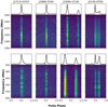 |
Fig. 1. Collage of the frequency evolution seen in the pulse profiles of the four pulsars presented in this work, along with their frequency averaged profiles. Top panel: data from BAND5 and bottom panel: BAND3 data. The data for the plot were obtained after adding high S/N observations from several epochs together using the known ephemeris of each pulsar. |
Summary of the observations used in this work.
3. Data analysis
The data folded with DSPSR after removing the RFIs using RFIClean are directly used for estimating the DM. Due to the limited time span of the dataset (∼1 year), it is not possible to obtain a reliable timing solution from these data. Hence, we used the latest parameter files published by the NANOGrav collaboration in their 12.5-year data release (Alam et al. 2021) for estimating DM. The first requirement for obtaining a high precision DM measurement using wide-band data like ours is to obtain a frequency-resolved high S/N template and aligning the sub-band profiles properly so that there is no residual DM delay in the template. If this correction is not done properly, the DMs estimated using such a template will be biased. We used two different methods to align the sub-band profiles in the template to check their effectiveness on the DM measurements as described in Sect. 3.1. We used these frequency-resolved templates to obtain ToAs and measure DM using TEMPO2 (Hobbs et al. 2006). A Python-based script, DMcalc was developed for this purpose using the PSRCHIVE tools. We also implemented an outlier rejection algorithm for removing large outlier ToAs using Huber Regression (Huber 1964) following Tiburzi et al. (2019). Details of our DM measurements are given in Sect. 3.2.
3.1. Selection of the template and their alignment
In our first method (METHOD1), we selected an epoch where the S/N (obtained using the pdmp program of PSRCHIVE) of the observation is comparatively high at both bands (BAND3 and BAND5). We estimated the DM at BAND3 using the pdmp program. Although the precision with which pdmp reports the DM is not very high, it is sufficient to align the sub-band profiles well in most cases. If the precision in the DM measurement reported by pdmp is worse than the change in DM from the ephemeris (with which the data are dedispersed), we did not update the DM (this is the case with PSR J1909−3744). The obtained DM is then used to dedisperse both BAND3 and BAND5 data. Smoothed templates were created from these files with the psrsmooth program in PSRCHIVE using the wavelet smoothing algorithm (Demorest et al. 2013). These smoothed templates were later used to estimate the DM.
It is possible that METHOD1 could bias the DM measurements as the alignment of the templates is performed using the pdmp DM, which tries to maximise the S/N while obtaining the best DM. To circumvent this issue, we employed a different method (METHOD2) for alignment, using an analytic template derived from the data. To do this, for every pulsar, we co-added the highest S/N observations in both bands using psradd to create one final fiducial dataset. A frequency-averaged as well as a time-averaged profile was produced from this co-added data in BAND3. We then used the PSRCHIVE tool paas to create an analytic template by fitting a mixture of Gaussians to this BAND3 profile. The noise-free analytic template created with this best fit was then used to estimate the DM of the aforementioned co-added dataset with DMcalc. The sub-banded profiles in the high S/N data were then aligned using the DM obtained from DMcalc, in both bands. We then used psrsmooth (similar to METHOD1), to obtain a noise-free frequency-resolved template using the DM-corrected co-added data. The frequency-resolved templates produced using both these methods were then used to obtain the DM time series, as described in the next subsection.
The DMs obtained using METHOD2 have, in general, an order of magnitude better uncertainties than the ones obtained with METHOD1. We also note that, in some cases, the actual DM value obtained using the two methods were slightly different. Additionally, it is possible for METHOD2 to give a biased DM for pulsars that show significant profile component evolution within the band as the initial alignment is obtained using a frequency-averaged profile.
3.2. Measurement of the DM
To measure the DM, we used frequency-resolved templates prepared as explained in Sect. 3.1. This approach removes the need for fitting other frequency-dependent parameters while fitting for DM as the pulsar profile shape at a given frequency remains very much invariant (except for mode changes or scattering variations). The DMs reported in this paper are obtained using the TEMPO2 package. We made use of the Python interface of PSRCHIVE for obtaining the ToAs and also for removing the outliers. Most of the data processing was performed with this Python interface, except for obtaining the ToA residuals and for the fitting of the DM, which were performed using TEMPO2. The procedure for performing the outlier rejection we use here closely follows that by Tiburzi et al. (2019). A Python-based tool named DMcalc4 was developed for performing the above operations.
We used the latest parameter files published by Alam et al. (2021) for obtaining the DM. We removed the DM and the DMX parameters from the parameter files as this could otherwise bias the measured DM values. FD parameters were also removed as we perform frequency-resolved ToA estimation in this work. We also kept the electron density due to the solar wind (NE_SW) as zero so as to remove bias. The DM in the parameter file was updated to the one that is obtained using either METHOD1 or METHOD2 for use in both the methods. The ToAs with the given frequency resolution for each pulsar were obtained at both bands by using the ArrivalTime class of PSRCHIVE available with the Python interface. We used the classical Fourier phase shift estimation method (Taylor 1992) implemented in PSRCHIVE as PGS for obtaining the ToAs. The ToAs thus obtained were then used to obtain frequency-resolved timing residuals using the general2 plugin of TEMPO2. A fit of ν−2, where ν is the barycentric frequency of the ToAs was performed to these residuals using Huber Regression (Huber 1964). A robust median absolute deviation (MAD) of the ToA residuals after removing the above fit from the residuals is calculated and the ToAs beyond three times the MAD value on both sides of the ToA residuals were removed. This outlier rejection method is effective in removing the large outliers that are otherwise present due to RFI or other issues in the data (for example, scintillation will make data of some channels almost unusable due to a very low S/N), which will corrupt the DMs obtained. These filtered ToAs were then used to fit for DM with TEMPO2.
An example analysis plot of PSR J2145−0750 is shown in Fig. 2. In this particular fit, we used a total of 16 sub-band profiles across the available 100 MHz bandwidth. The top two sub-bands were removed from the template as they were contaminated by RFI at most of the epochs. A total of 14 ToAs were obtained, one of which was rejected based on the outlier rejection criteria discussed above. A fit for DM was performed and the resulting ToAs after removing the DM trend can be found at the bottom-right panel of the figure. The pre-fit and post-fit weighted rms can be found at the top of the panel, in addition to other parameters. As can be seen from the figure, the weighted rms improved after fitting for the DM and its value is close to the median ToA uncertainty.
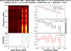 |
Fig. 2. Sample analysis plot of DMcalc using the observation of PSR J2145−0750 at BAND3 on 24 February 2019, when an excess DM was seen towards this pulsar (see Sect. 4 for the discussion). Details of the fit can be found at the top of the plot. Right panel: the top plot shows the pre-fit residuals obtained from TEMPO2 as grey circles and the Huber Regression fit to it as a dashed line in red. Middle panel: pre-fit ToAs after removing the outliers. Bottom panel: ToAs after fitting for DM using TEMPO2. The details of the analysis method can be found in Sect. 3.2. Left panel: the top panel shows an image of the frequency spectra of the pulse profiles of a 25 min observation after applying the DM correction and the bottom shows the frequency and time averaged profile of the observation. Source: PSR J2145−0750; MJD: 58538.2306; Prefit Wrms: 17.71 μs; Postfit Wrms: 6.35 μs; Median ToA Err: 7.31 μs; DM: 9.010648 ± 0.000578 pc cm−3; Reduced χ2: 0.50. |
This process is performed at BAND3 and BAND5 separately as well as in a combined BAND3 + BAND5 mode to obtain DMs. In the combined BAND3 + BAND5 mode, the data, as well as the templates of both bands, were combined with the modified pulsar ephemeris from Alam et al. (2021) using the FrequencyAppend() function available in the PSRCHIVE Python interface. The addition of the data without the requirement of having any jumps between the two bands is justified as these were observed simultaneously using the same receiver chain and processed identically in the uGMRT correlator, which synchronises all antenna data using a one pulse per second clock signal from the observatory’s active hydrogen maser. The relative delay was experimentally determined to be zero up to a precision of 5 ns using engineering tests (Susobhanan et al. 2021). The procedure was then repeated for all the observations to obtain the DM time series as shown in Fig. 3. In the case of inter-band DM measurements, the data of both bands were aligned using the pulsar ephemeris before obtaining the ToAs and DM.
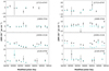 |
Fig. 3. DM time series after subtracting the median DM obtained from the BAND3 and BAND5 combined data as shown in Table 2 of the pulsars presented in this work. Left panel: DM time series obtained by METHOD1. Right panel: DM time series obtained by METHOD2. Black filled circles represent DM obtained from BAND3 and Cyan triangles indicate DM obtained by combining bands 3 and 5. The median DM obtained from combining the two bands (refer to Table 2) are subtracted from the DM values to produce this plot. The DMs obtained with only using BAND5 data are not shown in the plot as their uncertainties are large. |
The four pulsars presented in this work have different frequency evolution of their parameters like flux density, profile shapes, scintle sizes and scatter broadening. To illustrate this, frequency-resolved profiles for all four pulsars are shown in Fig. 1. As a result, we had to obtain ToAs with different frequency resolution for each of them as described in Sect. 4.
4. Results and discussions
The DM time series obtained using the methods described in Sect. 4 for the four pulsars are shown in Fig. 3. The left panel shows the DM measured using METHOD1 and the right panel shows DM obtained using METHOD2. The median DM values and their uncertainties for the four pulsars are listed in Table 2. We have only reported the measurements for which a reduced χ2 < 10 is obtained with TEMPO2. Some epochs show reduced χ2 values worse than 10, but looking at each of them individually showed that they were affected by heavy RFI. Although we put a higher limit on χ2 for getting the good measurements, most of them have reduced χ2 much less than 10 and close to 1. The median value of the DMs estimated using METHOD1 and METHOD2 differs slightly for PSRs J1713+0747 and J1909−3744, while there is a clear offset between the DMs for PSRs J1939+2134 and J2145−0750. The possible cause of this difference is the underlying difference in the profile alignment methods used.
Median values of ToA uncertainties and DM.
In the present work, we have used the data obtained by observing simultaneously at both BAND3 and BAND5 using a 100 MHz bandwidth. The fractional bandwidth at BAND5 is a factor of ∼4−5 smaller than those used by most of the other PTAs, which reduces the precision with which we can obtain DM at BAND5. But a better fractional bandwidth at BAND3 enables us to get a good handle on the DM. The DM precision we can obtain in general by using this dataset with the BAND3 data alone is ∼10−3 and while combining the two bands it gets better by an order of magnitude to ∼10−4. In particular, we achieve an order of magnitude better precision of 10−4 with BAND3 and 10−5 with BAND3 and BAND5 for PSR J1939+2134. Combining the two widely separated bands for measuring DM can create a bias due to the slightly different IISM the rays of these two bands pass through (Cordes et al. 2016).
Comparing our results obtained using the two methods described in this work to that of the recently published ones by Alam et al. (2021) and Donner et al. (2020) show interesting trends. For two pulsars, J1713+0747 and J2145−0750, we have data in both these datasets for comparison with ours. It should be noted that the data available from NANOGrav stops before our observations began whereas the data from Donner et al. (2020) covers this gap as well as extends beyond our dataset. For J1713+0747, we find our results from both methods to be consistent with the results from Donner et al. (2020), whereas it shows a small increase in DM of ∼2 × 10⁻³ pc cm−3 from NANOGrav results. For J2145−0750, the DM from METHOD1 shows a difference of ∼8 × 10⁻³ pc cm−3, whereas the ones obtained with METHOD2 show consistency with the other two datasets. For J1909−3744 and J1939+2134, we only have DM measurements from NANOGrav to compare, although the datasets do not overlap each other. For J1909−3744, the template DMs used for both methods are different due to their inherent differences in obtaining it. A difference of ∼2 × 10⁻³ pc cm−3 in the DM applied in the template caused the difference in the obtained DM using our two methods. Both of these measurements will have a small bias if the NANOGrav DM time series is extrapolated to cover our epochs. For J1939+2134, both alignment methods, METHOD1 as well as METHOD2, could create a bias due to scattering. A completely different method taking care of the scattering evolution for each observation has to be used in such a case, which will be taken up in a follow-up work. In summary, both these alignment methods can be useful in getting DMs, but a systematic bias could be possible in either of the methods, which will be very much pulsar specific. Below we discuss in detail the results of each of the pulsars studied in this paper.
4.1. PSR J1713+0747
This is one of the most precisely timed pulsars in PTA datasets. We did not detect this pulsar at some epochs. This could be due to the effect of diffractive scintillation affecting the luminosity at each epoch as the number of scintles available in the band becomes close to 1 (Cordes & Lazio 1991; Cordes & Chernoff 1997). Assuming a scintillation bandwidth of 20 MHz and scintillation time of 45 min (Keith et al. 2013; Levin et al. 2016), the number of available scintles in the band at a given time will be 1−3. In this low number regime, the pulse intensity is expected to be 100% modulated (Cordes & Lazio 1991), causing the S/N to be below our detection sensitivity at some epochs. This essentially reduced our DM precision at BAND5 and also made some of the observations essentially unusable for our analysis. We collapsed the data to 16 channels at both bands for obtaining the DMs. Both methods give similar DMs at both bands, but the combined estimate shows a small bias. The DMs used for aligning the templates using both the methods are slightly different, by ∼0.01 pc cm−3. From Fig. 3, it can be seen that the DM measurements at some epochs are missing in the left panel. This is because the reduced χ2 of those fits are beyond the cutoff value and were removed from the plot. The average DM obtained in this work is consistent with that obtained by Donner et al. (2020) using LOFAR data, but is slightly higher than the DMs obtained by Alam et al. (2021) by about 2 × 10⁻³ pc cm−3. This small bias from Alam et al. (2021) could be due to the frequency dependence of the DM (or scattering) as both BAND3 and LOFAR frequency bands are close to each other. The median ToA precision obtained at BAND5 is close to 1 μs.
4.2. PSR J1909−3744
Similar to the previous pulsar, this one is also a precisely timed pulsar with PTAs. Here also we collapsed the data to 16 channels at both bands for DM measurement. The average DM obtained using the two methods, after combining the two bands show a slight difference. This small bias, as in the previous case, could be due to the initial DM used for aligning the templates (they differ by 3 × 10⁻³ pc cm−3). The pulse shape remains the same (without any major profile evolution) at both BAND3 and BAND5. It is possible that we are unable to detect any small profile evolution due to the coarse sampling of the pulse phase. This prevented us from getting a better analytic profile for obtaining the DM with which the template was aligned. The DM time series reported in Alam et al. (2021) does not cover the epochs of our observations, but extrapolating their measurements to ours show a better alignment with the DMs obtained using METHOD1 and a small difference of ∼2 × 10⁻³ pc cm−3 with that of METHOD2, as evident from the difference in their average DMs. The ToA precision is similar in both bands.
4.3. PSR J1939+2134
This is one of the longest timed MSPs by all the PTAs (Kaspi et al. 1994; Verbiest et al. 2016). It shows timing noise in its ToA residuals and its timing data cannot be used for GW analysis without proper noise modelling. Since the pulsar is one of the brightest MSPs in our set, the precision in DM that can be achieved is quite high. Due to this, we used 128 channels at BAND3 and 32 channels at BAND5 in the DM analysis. One limitation this pulsar has for using the BAND3 data for estimating DM is that it has very strong scatter broadening. Due to this reason, the initial DM obtained by the two different methods we used differ by about ∼6 × 10⁻³ pc cm−3. This is exactly the difference between the average DMs reported in Table 2 for the combined bands. There is a small difference of ∼5 × 10⁻⁴ pc cm−3 between the BAND3 DMs and the combined ones obtained using METHOD2. This is probably due to the presence of scattering at BAND3. The DM obtained using both methods show differences even after taking these biases into account. This indicates that the scatter broadening present in the pulsar signal is also time-varying. A proper analysis of scatter broadening and simultaneous measurement of DM is required to disentangle the DM getting biased by the extra delay caused by scattering. This will be taken up in a future study. The DM time series obtained using METHOD1 follows the trend seen in Alam et al. (2021), although the DMs reported here suffer from scattering bias. The ToA precision we obtain is the best for this pulsar in our sample, which is also indicative of the DM precision we could achieve.
4.4. PSR J2145−0750
This is one of the brightest pulsars in our sample. It shows a strong profile evolution across both of the bands. Moreover, this pulsar’s line of sight passes close to the Sun at a solar elongation of ∼5°. It has been reported previously that the DM shows an increase due to the increase in the heliospheric electron density (solar wind) as its line of sight approaches close to the Sun (Kumar et al. 2013; Alam et al. 2021; Donner et al. 2020; Tiburzi et al. 2021). Since this pulsar has several scintles in BAND3 data, we collapsed it to 16 channels to reduce the effect of scintillation. At BAND5, we used 8 channels across the band. The median DMs obtained using the two methods shown in Table 2 differ by about 1.1 × 10⁻² pc cm−3 for the combined bands. Even though the S/N of the data used for generating the template was good, the precision in DM using METHOD1 is worse than the difference quoted above. This is possibly due to change in relative amplitudes of profile components with frequency, which increases uncertainty while maximising S/N in pdmp. This is not an issue for METHOD2, which obtained a precision in the fourth decimal place for the profile alignment using the analytic template. Although this creates a constant bias between the DM time series obtained using the two methods, the trend in it is not much affected as can be seen in Fig. 3. The DMs obtained with METHOD2 show better alignment with the ones from Alam et al. (2021) and Donner et al. (2020), while the ones obtained with METHOD1 have an offset. The median ToA precision we could obtain is about 4 μs at BAND5.
Since the line of sight to this pulsar passes close to the Sun (between January and March), we compare the observed DM time series as a function of solar elongation (obtained from TEMPO2 as solarangle; You et al. 2007) as shown in Fig. 4. The red curve in the figure shows the expected DM excess caused by the background solar wind as predicted by the model incorporated in TEMPO2. We have only two observations as the line of sight to the pulsar passed close to the Sun, respectively, at solar elongations ∼5 and ∼10°. In Fig. 4, it is seen that the DM measurement on 10 February 2019 (MJD: 58524) at a solar elongation of ∼5° shows nominal increase and it is consistent with the value expected from the model, whereas the other measurement at about 10° (i.e. a radial distance of ∼40 solar radii) away from the Sun on 24 February 2019 (MJD: 58538) shows a DM excess of about an order of magnitude higher than the model. The DMcalc fit for this excess DM observed is shown in Fig. 2. To find the cause of this excess DM, we carefully examined the various solar datasets and solar wind measurements available during this epoch.
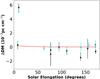 |
Fig. 4. DM time series of PSR J2145−0750 plotted as a function of solar elongation after subtracting the median DM value. The colour scheme is the same as in Fig. 3. The red line shows the expected DM excess by the solar wind as obtained from TEMPO2. |
The examination of solar images from the Solar Dynamic Observatory (SDO; Pesnell et al. 2012) revealed the onsets of two eruptions, i.e. CMEs at ∼10° west of the Sun’s centre between 03 and 24 UT on 23 February 2019. The ahead spacecraft of the Solar TErrestrial RElations Observatory (STEREO-A; Kaiser et al. 2008) was located 99° east of the Sun-Earth line and it observed the above eruptions at about 20° behind the west limb of the Sun. Since these CMEs originated close to the disk centre and were relatively narrow, they did not fill and show their expansion outside the field of view of the occulting disk of the coronagraph at the near-Earth spacecraft. In addition to these CMEs, the SDO images showed the presence of a large coronal hole ∼30° wide, extending from the origin of the CME to the east nearly along the equatorial region of the Sun. The high-speed streams from the coronal hole were likely to interact with the low-speed solar wind as well as CMEs.
Figure 5 shows the typical geometry of the line of sight to the pulsar with respect to the Sun, the possible propagation direction of CMEs, and slow solar wind along the Parker (Archimedean) spiral. The analysis of the interplanetary magnetic field and solar wind plasma from the OMNI datasets revealed an interplanetary shock at 07:35 UT on 27 February associated with the interaction between the slow- and high-speed solar wind streams. Figure 6 shows a 3-day period solar wind and interplanetary magnetic field measurements from 26 to 28 February 2019, obtained from the OMNI database5. From top to bottom, the figure shows the solar wind proton density, velocity, temperature, the magnitude of interplanetary magnetic field and plasma beta (β). The arrival of the shock is indicated by a vertical dotted line. The average ambient solar wind speed of ∼300 to 350 km s−1, observed during the latter half of February 2019, suggests that the interaction by the high-speed streams of speed ∼600 to 650 km s−1, would have been formed and developed well ahead of its arrival at the Earth. The shock was followed by an intense interaction region, which was more than an order of magnitude denser than the ambient solar wind as well as about a half day wide in time. In the interaction region, the magnetic field exhibited large intensity fluctuations and the plasma beta, which is the ratio between the gas and magnetic pressures, also showed a large peak. The temperature, density and velocity measurements after the interaction region showed clear characteristics of the streams from the coronal hole. The backward projection of the interaction region suggests that the interaction would have crossed the pulsar line of sight on 24 February around 2 to 8 UT.
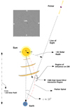 |
Fig. 5. Sketch of the geometry of the line of sight to the pulsar with respect to the Sun on 24 February 2019. The interaction region with excess electrons can be large in size while crossing the line of sight. The inset image shown at the top is the running difference EUV image of the Sun taken at 03:32 UT on 23 February 2019 by the SDO AIA telescope at 171 Å. |
In the case of the ambient solar wind, the density decay with the distance from the Sun can be considered to be R−2, typical for a spherically symmetric expansion of the solar wind, where R is the heliocentric distance. However, when the high-density solar wind structures, such CMEs and/or high-speed stream interactions are involved, a radial density gradient of R−2.5 or steeper has been observed (e.g. Bird et al. 1994; Elliott et al. 2012).
Assuming the R−2 relation, it can be estimated that this interaction region had a density of ∼1 × 103 cm−3, taking 45 cm−3 from the top panel of Fig. 6 as the density at Earth (1 AU). The above density enhancement was also confirmed by the NOAA/NASA/USAF Deep Space Climate Observatory space mission6. This density region (assuming the same extent of the interaction region at 41 solar radii) will create an excess DM of 1 × 10⁻³ pc cm−3. If we assume the steeper density gradient of R−2.5, a DM excess of 3 × 10⁻³ pc cm−3 can be obtained. Another point to be considered is that the eastern side of the interaction region likely crossed the Earth and it was possibly a little less dense than the nose of the interaction region, as indicated by the in situ measurements. Thus, the excessive DM observed probably corresponds to the density enhancement caused by the interactions between high-speed and low-speed solar wind and CMEs.
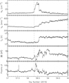 |
Fig. 6. In situ measured 5-min averaged OMNI data for a 3-day period, from 26 to 28 February 2019, during the passage of interaction region associated with the high-speed solar wind streams and slow CME or ambient wind. From the top to bottom: following data are plotted: solar wind proton density (Np), velocity (Vp), temperature (Tp), magnitude of the interplanetary magnetic field (|B|) and plasma beta (β). The vertical dashed line indicates the arrival of the interplanetary shock associated with the interaction region. The time immediately after the shock shows the intense interaction region, which is followed by the clear signatures of the high-speed streams from the coronal hole. The data used in this plot are obtained from the OMNI database at https://omniweb.gsfc.nasa.gov. |
A similar CME event was reported on PSR B0950+08 by Howard et al. (2016) and also possibly on PSR J1614−2230 by Madison et al. (2019). The solar wind stream interactions as well as stream-CME interactions are expected when the Sun is dominated by the mid-latitude and equatorial coronal holes. The vast sets of PTA and other pulsar observations available are likely to include many such events. A coordinated analysis of selected datasets would be of interest in understanding the effects of enhanced density structures of the solar wind on the DM variations as functions of solar offset and possibly also the phase of the solar cycle.
5. Summary and conclusions
In this paper, we compared the two possible methods for aligning the frequency-resolved pulsar profile templates and probed their effects on the resulting DM measurements. We used four InPTA pulsars observed by the uGMRT for a period of a year (two observing cycles at GMRT). These observations were done simultaneously at BAND3 and BAND5 of uGMRT with a 100 MHz bandwidth. For a uniform and systematic processing, we have developed a Python-based tool, DMcalc, utilising the PSRCHIVE Python interface and TEMPO2 for estimating DM using the templates from the above two methods. We regularly obtained a DM precision of ∼10−3 pc cm−3 at BAND3 and ∼10−4 pc cm−3 when combining it with BAND5 data while using both of our template alignment methods.
We find that both the methods are useful for aligning the templates, but METHOD2 could show a constant bias if the pulsar has scatter broadening. For pulsars that have no detectable scatter broadening, the DMs obtained by METHOD1 show a consistent bias from that obtained with METHOD2. This is essentially due to the use of two different methods for template alignment. METHOD1 uses an algorithm that aligns the multi-channel data by maximising the S/N while METHOD2 uses an analytic model derived from the frequency averaged profile of the data.
We have compared the DMs obtained by these two methods with the other recently published results (Alam et al. 2021; Donner et al. 2020). Our DM measurements for PSRs J1713+0747 and J2145−0750 using METHOD2 compare very well with theirs, while those from METHOD1 show a bias. In the cases of PSRs J1909−3744 and J1939+2134, our data have no overlap with either of the published datasets. Nevertheless, we see a continuing trend of the NANOGrav DM time series for J1939+2134 using METHOD1, while METHOD2 shows a clear constant offset. An improved method that takes care of the scattering bias while estimating the DM will be able to remove any bias created by scattering. For J1909−3744, we expect to see a small offset from that of the NANOGrav data using both methods, although the DMs obtained with METHOD1 may have smaller bias than the other.
In addition to the DM offset introduced due to different template alignment methods, there could be other contributing factors for the DM offset that we have not been accounted for in this work. One of the main causes for the offset between our DMs and the ones in the literature (Alam et al. 2021; Donner et al. 2020) is due to scattering (at least for PSR J1939+2134). Scatter-broadening introduces an extra delay in the ToAs and it scales as ν−4. Furthermore, if the delay varies over time, it could corrupt the trend in the DM time series of the pulsar. Currently neither of our methods take that into account and this will be taken up in a future work. The DM obtained from combining the data from the two widely separated bands could also get affected by the profile evolution. Although we do not see such an offset in our data yet, given the coarse phase resolution, it is possible that we may have to take that into account when the phase resolution improves in future datasets. The DM obtained from combining the data from the two widely separated bands could also be affected by the profile evolution. Given the coarse phase resolution in our data, we currently do not see such an offset. However, it will have to be accounted for in future data with finer phase resolution. It was suggested by Cordes et al. (2016) that the DM is frequency dependent. This means that a possible offset could be introduced when these widely separated frequency bands are combined. Although we do not see any evidence for this with the current dataset, it could become evident with better datasets in the future.
Our data are in total intensity mode and hence there is no polarisation information available. This could affect the alignment of the combined BAND3 + BAND5 data. But our coarse pulse phase resolution and lack of full Stokes data makes it difficult to either confirm or rule it out.
We could obtain a ToA precision of ∼1μs or better for all pulsars in both the bands, which is highly encouraging. We see the effect of scattering on DM measurements of J1939+2134. In a follow-up study, we plan to disentangle the two effects to obtain better DM estimates.
We infer that the DM measurement at MJD 58538 of PSR J2145−0750 with a solar elongation of ∼10° was enhanced by an interaction region formed by a CME and high-speed solar wind from a coronal hole close to the origin of the CME. Similar events can be of interest to both the pulsar and the solar wind community and our results show that such studies can be pursued using high precision data from the uGMRT.
The present observations used a 20−25 min scan for each pulsar. A much better precision on both ToAs and hence DM can be achieved by using longer integrations and wider bandwidths of the uGMRT. We started doing observations using a bandwidth of 200 MHz at both BAND3 and BAND5 simultaneously and also increased the observation duration in addition to increasing the number of antennas at each band (by skipping BAND4, and utilising the antennas at the other two bands). A factor of three improvement in the precision of DM is expected at BAND3 in general with this increased bandwidth as compared to current results. Initial results show vast improvement in the S/N of the pulsars. The data from these observations are under various stages of processing and will be reported elsewhere.
Following the encouraging results from the work presented here, we plan to apply these techniques to our full sample of pulsars observed during the last four years. Additionally, efforts are being pursued for developing other methods to make the DM measurements even more precise and reliable, and therefore employable for the ongoing gravitational wave analysis by the various PTAs.
Acknowledgments
MAK is thankful to Caterina Tiburzi and Joris Verbiest for their valuable inputs and useful discussions at various stages of this work. We are thankful to the anonymous referee for many constructive comments on the manuscript. AS, AG, BCJ, LD, and YG acknowledge the support of the Department of Atomic Energy, Government of India, under project Identification # RTI 4002. BCJ, YG, and AB acknowledge support from the Department of Atomic Energy, Government of India, under project # 12-R&D-TFR-5.02-0700. AC acknowledges support from the Women’s Scientist scheme (WOS-A), Department of Science and Technology, India. MPS acknowledges funding from the European Research Council (ERC) under the European Union’s Horizon 2020 research and innovation programme (grant agreement No. 694745). NDB acknowledges support from the Department of Science & Technology, Government of India, grant SR/WOS-A/PM-1031/2014. AB acknowledges the support from the UK Science and Technology Facilities Council (STFC). Pulsar research at Jodrell Bank Centre for Astrophysics and Jodrell Bank Observatory is supported by a consolidated grant from STFC. We thank the staff of the GMRT who made our observations possible. GMRT is run by the National Centre for Radio Astrophysics of the Tata Institute of Fundamental Research. The open data policy of STEREO and SDO teams is acknowledged. The solar wind and interplanetary datasets have been obtained from the OMNI database.
References
- Ahuja, A. L., Gupta, Y., Mitra, D., & Kembhavi, A. K. 2005, MNRAS, 357, 1013 [NASA ADS] [CrossRef] [Google Scholar]
- Ahuja, A. L., Mitra, D., & Gupta, Y. 2007, MNRAS, 377, 677 [NASA ADS] [CrossRef] [Google Scholar]
- Alam, M. F., Arzoumanian, Z., Baker, P. T., et al. 2021, ApJS, 252, 5 [CrossRef] [Google Scholar]
- Arzoumanian, Z., Baker, P. T., Blumer, H., et al. 2020, ApJ, 905, L34 [CrossRef] [Google Scholar]
- Backer, D. C. 1996, in Compact Stars in Binaries, eds. J. van Paradijs, E. P. J. van den Heuvel, & E. Kuulkers, 165, 197 [CrossRef] [Google Scholar]
- Bird, M. K., Volland, H., Paetzold, M., et al. 1994, ApJ, 426, 373 [Google Scholar]
- Burke-Spolaor, S., Taylor, S. R., Charisi, M., et al. 2019, A&ARv, 27, 5 [Google Scholar]
- Cordes, J. M., & Chernoff, D. F. 1997, ApJ, 482, 971 [NASA ADS] [CrossRef] [Google Scholar]
- Cordes, J. M., & Lazio, T. J. 1991, ApJ, 376, 123 [NASA ADS] [CrossRef] [Google Scholar]
- Cordes, J. M., Shannon, R. M., & Stinebring, D. R. 2016, ApJ, 817, 16 [Google Scholar]
- De, K., & Gupta, Y. 2016, Exp. Astron., 41, 67 [CrossRef] [Google Scholar]
- Demorest, P. B., Ferdman, R. D., Gonzalez, M. E., et al. 2013, ApJ, 762, 94 [Google Scholar]
- Desvignes, G., Caballero, R. N., Lentati, L., et al. 2016, MNRAS, 458, 3341 [Google Scholar]
- Donner, J. Y., Verbiest, J. P. W., Tiburzi, C., et al. 2019, A&A, 624, A22 [NASA ADS] [CrossRef] [EDP Sciences] [Google Scholar]
- Donner, J. Y., Verbiest, J. P. W., Tiburzi, C., et al. 2020, A&A, 644, A153 [EDP Sciences] [Google Scholar]
- Edwards, R. T., Hobbs, G. B., & Manchester, R. N. 2006, MNRAS, 372, 1549 [Google Scholar]
- Elliott, H. A., Henney, C. J., McComas, D. J., Smith, C. W., & Vasquez, B. J. 2012, J. Geophys. Res.: Space Phys., 117, A09102 [NASA ADS] [Google Scholar]
- Foster, R. S., & Backer, D. C. 1990, ApJ, 361, 300 [NASA ADS] [CrossRef] [Google Scholar]
- Gupta, Y., Ajithkumar, B., Kale, H. S., et al. 2017, Curr. Sci., 113, 707 [NASA ADS] [CrossRef] [Google Scholar]
- Hobbs, G. 2013, Classical Quantum Gravity, 30, 224007 [NASA ADS] [CrossRef] [Google Scholar]
- Hobbs, G. B., Edwards, R. T., & Manchester, R. N. 2006, MNRAS, 369, 655 [Google Scholar]
- Hobbs, G., Guo, L., Caballero, R. N., et al. 2019, MNRAS, 491, 5951 [CrossRef] [Google Scholar]
- Hotan, A. W., van Straten, W., & Manchester, R. N. 2004, PASA, 21, 302 [Google Scholar]
- Howard, T. A., Stovall, K., Dowell, J., Taylor, G. B., & White, S. M. 2016, ApJ, 831, 208 [CrossRef] [Google Scholar]
- Huber, P. J. 1964, Ann. Math. Stat., 35, 73 [CrossRef] [Google Scholar]
- Joshi, B. C., Arumugasamy, P., Bagchi, M., et al. 2018, JApA, 39, 51 [Google Scholar]
- Kaiser, M. L., Kucera, T. A., Davila, J. M., et al. 2008, Space Sci. Rev., 136, 5 [NASA ADS] [CrossRef] [Google Scholar]
- Kaspi, V. M., Taylor, J. H., & Ryba, M. F. 1994, ApJ, 428, 713 [NASA ADS] [CrossRef] [Google Scholar]
- Kaur, D., Bhat, N. D. R., Tremblay, S. E., et al. 2019, ApJ, 882, 133 [CrossRef] [Google Scholar]
- Keith, M. J., Coles, W., Shannon, R. M., et al. 2013, MNRAS, 429, 2161 [NASA ADS] [CrossRef] [Google Scholar]
- Kerr, M., Reardon, D. J., Hobbs, G., et al. 2020, PASA, 37, e020 [CrossRef] [Google Scholar]
- Kramer, M., & Champion, D. J. 2013, Classical Quantum Gravity, 30, 224009 [NASA ADS] [CrossRef] [Google Scholar]
- Kumar, U., Gupta, Y., van Straten, W., et al. 2013, in Neutron Stars and Pulsars: Challenges and Opportunities after 80 Years, ed. J. van Leeuwen, 291, 432 [Google Scholar]
- Levin, L., McLaughlin, M. A., Jones, G., et al. 2016, ApJ, 818, 166 [CrossRef] [Google Scholar]
- Liu, K., Desvignes, G., Cognard, I., et al. 2014, MNRAS, 443, 3752 [NASA ADS] [CrossRef] [Google Scholar]
- Lorimer, D., & Kramer, M. 2004, Handbook of Pulsar Astronomy (Cambridge: Cambridge University Press) [Google Scholar]
- Maan, Y., van Leeuwen, J., & Vohl, D. 2021, A&A, 650, A80 [CrossRef] [EDP Sciences] [Google Scholar]
- Madison, D. R., Cordes, J. M., Arzoumanian, Z., et al. 2019, ApJ, 872, 150 [Google Scholar]
- McLaughlin, M. A. 2013, Classical Quantum Gravity, 30, 224008 [NASA ADS] [CrossRef] [Google Scholar]
- Perera, B. B., DeCesar, M. E., Demorest, P. B., et al. 2019, MNRAS, 490, 4666 [NASA ADS] [CrossRef] [Google Scholar]
- Pesnell, W. D., Thompson, B. J., & Chamberlin, P. C. 2012, Sol. Phys., 275, 3 [Google Scholar]
- Reddy, S. H., Kudale, S., Gokhale, U., et al. 2017, J. Astron. Instrum., 6, 1641011 [CrossRef] [Google Scholar]
- Susobhanan, A., Maan, Y., Joshi, B. C., et al. 2021, PASA, 38, e017 [Google Scholar]
- Swarup, G., Ananthakrishnan, S., Kapahi, V. K., et al. 1991, Curr. Sci., 60, 95 [Google Scholar]
- Taylor, J. H. 1992, Philos. Trans. R. Soc. London Ser. A, 341, 117 [NASA ADS] [CrossRef] [Google Scholar]
- Tiburzi, C., Verbiest, J. P. W., Shaifullah, G. M., et al. 2019, MNRAS, 487, 394 [Google Scholar]
- Tiburzi, C., Shaifullah, G. M., Bassa, C. G., et al. 2021, A&A, 647, A84 [CrossRef] [EDP Sciences] [Google Scholar]
- van Straten, W., & Bailes, M. 2011, PASA, 28, 1 [Google Scholar]
- Verbiest, J. P. W., Lentati, L., Hobbs, G., et al. 2016, MNRAS, 458, 1267 [Google Scholar]
- You, X. P., Hobbs, G. B., Coles, W. A., Manchester, R. N., & Han, J. L. 2007, ApJ, 671, 907 [Google Scholar]
All Tables
All Figures
|
Fig. 1. Collage of the frequency evolution seen in the pulse profiles of the four pulsars presented in this work, along with their frequency averaged profiles. Top panel: data from BAND5 and bottom panel: BAND3 data. The data for the plot were obtained after adding high S/N observations from several epochs together using the known ephemeris of each pulsar. |
| In the text | |
|
Fig. 2. Sample analysis plot of DMcalc using the observation of PSR J2145−0750 at BAND3 on 24 February 2019, when an excess DM was seen towards this pulsar (see Sect. 4 for the discussion). Details of the fit can be found at the top of the plot. Right panel: the top plot shows the pre-fit residuals obtained from TEMPO2 as grey circles and the Huber Regression fit to it as a dashed line in red. Middle panel: pre-fit ToAs after removing the outliers. Bottom panel: ToAs after fitting for DM using TEMPO2. The details of the analysis method can be found in Sect. 3.2. Left panel: the top panel shows an image of the frequency spectra of the pulse profiles of a 25 min observation after applying the DM correction and the bottom shows the frequency and time averaged profile of the observation. Source: PSR J2145−0750; MJD: 58538.2306; Prefit Wrms: 17.71 μs; Postfit Wrms: 6.35 μs; Median ToA Err: 7.31 μs; DM: 9.010648 ± 0.000578 pc cm−3; Reduced χ2: 0.50. |
| In the text | |
|
Fig. 3. DM time series after subtracting the median DM obtained from the BAND3 and BAND5 combined data as shown in Table 2 of the pulsars presented in this work. Left panel: DM time series obtained by METHOD1. Right panel: DM time series obtained by METHOD2. Black filled circles represent DM obtained from BAND3 and Cyan triangles indicate DM obtained by combining bands 3 and 5. The median DM obtained from combining the two bands (refer to Table 2) are subtracted from the DM values to produce this plot. The DMs obtained with only using BAND5 data are not shown in the plot as their uncertainties are large. |
| In the text | |
|
Fig. 4. DM time series of PSR J2145−0750 plotted as a function of solar elongation after subtracting the median DM value. The colour scheme is the same as in Fig. 3. The red line shows the expected DM excess by the solar wind as obtained from TEMPO2. |
| In the text | |
|
Fig. 5. Sketch of the geometry of the line of sight to the pulsar with respect to the Sun on 24 February 2019. The interaction region with excess electrons can be large in size while crossing the line of sight. The inset image shown at the top is the running difference EUV image of the Sun taken at 03:32 UT on 23 February 2019 by the SDO AIA telescope at 171 Å. |
| In the text | |
|
Fig. 6. In situ measured 5-min averaged OMNI data for a 3-day period, from 26 to 28 February 2019, during the passage of interaction region associated with the high-speed solar wind streams and slow CME or ambient wind. From the top to bottom: following data are plotted: solar wind proton density (Np), velocity (Vp), temperature (Tp), magnitude of the interplanetary magnetic field (|B|) and plasma beta (β). The vertical dashed line indicates the arrival of the interplanetary shock associated with the interaction region. The time immediately after the shock shows the intense interaction region, which is followed by the clear signatures of the high-speed streams from the coronal hole. The data used in this plot are obtained from the OMNI database at https://omniweb.gsfc.nasa.gov. |
| In the text | |
Current usage metrics show cumulative count of Article Views (full-text article views including HTML views, PDF and ePub downloads, according to the available data) and Abstracts Views on Vision4Press platform.
Data correspond to usage on the plateform after 2015. The current usage metrics is available 48-96 hours after online publication and is updated daily on week days.
Initial download of the metrics may take a while.