| Issue |
A&A
Volume 651, July 2021
|
|
|---|---|---|
| Article Number | A59 | |
| Number of page(s) | 16 | |
| Section | Interstellar and circumstellar matter | |
| DOI | https://doi.org/10.1051/0004-6361/202040223 | |
| Published online | 13 July 2021 | |
The dense warm ionized medium in the inner Galaxy★
1
Jet Propulsion Laboratory, California Institute of Technology,
4800 Oak Grove Drive,
Pasadena,
CA
91109,
USA
e-mail: This email address is being protected from spambots. You need JavaScript enabled to view it.
2
SOFIA-USRA, NASA Ames Research Center,
MS 232-12,
Moffett Field,
CA
94035-0001,
USA
3
Max-Planck-Institut für Radioastronomie,
Auf dem Hügel 69,
53121
Bonn,
Germany
4
Department of Physics and Astronomy, West Virginia University,
Morgantown,
WV
26506,
USA
5
Center for Gravitational Waves and Cosmology, West Virginia University, Chestnut Ridge Research Building,
Morgantown,
WV
2605,
USA
6
Green Bank Observatory,
PO Box 2,
Green Bank,
WV
24944,
USA
7
I. Physikalisches Institut der Universität zu Köln,
Zülpicher Strasse 77,
50937
Köln,
Germany
Received:
23
December
2020
Accepted:
30
April
2021
Abstract
Context. Ionized interstellar gas is an important component of the interstellar medium and its lifecycle. The recent evidence for a widely distributed highly ionized warm interstellar gas with a density intermediate between the warm ionized medium (WIM) and compact H II regions suggests that there is a major gap in our understanding of the interstellar gas.
Aims. Our goal is to investigate the properties of the dense WIM in the Milky Way using spectrally resolved SOFIA GREAT [N II] 205 μm fine-structure lines and Green Bank Telescope hydrogen radio recombination lines (RRL) data, supplemented by spectrally unresolved Herschel PACS [N II] 122μm data, and spectrally resolved 12CO.
Methods. We observed eight lines of sight (LOS) in the 20° < l < 30° region in the Galactic plane. We analyzed spectrally resolved lines of [N II] at 205 μm and RRL observations, along with the spectrally unresolved Herschel PACS 122 μm emission, using excitation and radiative transfer models to determine the physical parameters of the dense WIM. We derived the kinetic temperature, as well as the thermal and turbulent velocity dispersions from the [N II] and RRL linewidths.
Results. The regions with [N II] 205 μm emission are characterized by electron densities, n(e) ~ 10−35 cm−3, temperatures range from 3400 to 8500 K, and nitrogen column densities N(N+) ~ 7 × 10¹⁶ to 3 × 1017 cm−2. The ionized hydrogen column densities range from 6 × 10²⁰ to 1.7 × 1021 cm−2 and the fractional nitrogen ion abundance x(N+) ~ 1.1 × 10⁻⁴ to 3.0 × 10⁻⁴, implying an enhanced nitrogen abundance at a distance ~4.3 kpc from the Galactic Center. The [N II] 205 μm emission lines coincide with CO emission, although often with an offset in velocity, which suggests that the dense warm ionized gas is located in, or near, star-forming regions, which themselves are associated with molecular gas.
Conclusions. These dense ionized regions are found to contribute ≳50% of the observed [C II] intensity along these LOS. The kinetic temperatures we derive are too low to explain the presence of N+ resulting from electron collisional ionization and/or proton charge transfer of atomic nitrogen. Rather, these regions most likely are ionized by extreme ultraviolet (EUV) radiation from nearby star-forming regions or as a result of EUV leakage through a clumpy and porous interstellar medium.
Key words: ISM: structure / ISM: abundances / HII regions
The spectral files in Fig. 2 are also available at the CDS via anonymous ftp to cdsarc.u-strasbg.fr (130.79.128.5) or via http://cdsarc.u-strasbg.fr/viz-bin/cat/J/A+A/651/A59
© ESO 2021
1 Introduction
The Galactic interstellar medium (ISM) cycles gas from a diffuse ionized state through succeedingly denser neutral components until dense molecular clouds form in which young stars are born. These stars and supernovae generate winds and radiation that disrupt the clouds and ionize the gas, continuing the cycle. The neutral atomic hydrogen and molecular hydrogen clouds occupy only a small volume of the Galactic disk, ~2%, compared to the ionized gas, which fills much of its volume. A significant fraction of the Galactic disk, ~20% to 40%, is filled with low density ionized hydrogen in a warm ionized medium (WIM), also called the diffuse ionized gas (DIG), with an average electron density ~0.03–0.08 cm−3 and Tkin ~ 8000 K (Haffner et al. 2009). The WIM/DIG is estimated to comprise ~90% of the ionized gas in the Galaxy and ~20% of the total gas mass (Reynolds 1991).
The low density WIM has been studied for nearly six decades since it was proposed as a component of the Galaxy’s ISM by Hoyle & Ellis (1963). Pulsar dispersion measurements, faint optical emission lines, and surveys in Hnα emission established that the WIM is widespread throughout the Galaxy (see review by Haffner et al. 2009), in contrast to H II regions with n(e) ≳ 102 cm−3. Bright denseH II regions are strong sources of emission of the fine structure far-infrared lines of ionized carbon, [C II], and nitrogen, [N II]. In contrast the WIM can only be detected in [C II] and [N II] in absorption towards bright continuum sources with these tracers of ionized gas (Persson et al. 2014; Gerin et al. 2015), or in emission along the tangent lines of spiral arms where a long column density of gas has a small velocity dispersion (Velusamy et al. 2012, 2015; Langer et al. 2017).
Thus, the discovery of dense warm ionized gas associated with molecular gas clouds in the inner disk (l = ±60°) of the MilkyWay (Goldsmith et al. 2015) was unexpected. Goldsmith et al. (2015) conducted a survey of [N II] 205 and 122 μm emission along ~150 lines of sight (LOS) in the plane using the Herschel PACS array and detected relatively strong emission as compared with predictions from the large scale and low angular resolution (~7°) COBE maps, which indicated that [N II], which arises solely from ionized hydrogen gas, was weak (Bennett et al. 1994). As originally shown by Rubin (1989), ionized nitrogen requires relatively high electron densities to excite its fine structure levels and would be difficult detect in the WIM with PACS. The PACS 122 and 205 μm intensities were used to derive the electron abundances and column densities of the ionized gas. The densities, n(e), were largely in the range 10–50 cm−3, intermediate between the low density WIM and H II regions with n(e) ≳ 102 cm−3, and much lower than ultracompact H II regions with n(e) > 103 cm−3 (Kurtz 2005). Here, we investigate the properties of the dense warm ionized gas along eight LOSs toward the inner Milky Way using spectrally resolved SOFIA GREAT [N II] 205 μm fine-structure lines and Green Bank Telescope (GBT) hydrogen radio recombination lines (RRL), supplemented by spectrally unresolved Herschel PACS [N II] 205 and 122 μm data, and CO spectra. From these data we derive the electron density and temperature, the N+ and H+ column densities, and fractional nitrogen ion abundance.
In the Herschel Galactic [N II] sparse survey, ten LOSs observed with PACS were also observed with spectrally resolved 205 μm emission with Herschel’s Heterodyne Instrument in the Far-Infrared (HIFI) and found to have ~20 distinct velocity components (Langer et al. 2016). Pineda et al. (2019) analyzed the electron abundance and column density of N+ in these 20 spectral components along with one in the Scutum arm l ~ 30° that had been observed in [N II] 205 μm with SOFIA GREAT (Langer et al. 2017). To derive the electron density, in the absence of spectrally resolved 122 μm [N II] emission, Pineda et al. (2019) developed a technique combining spectrally resolved Hnα RRLs with the spectrally resolved [N II] 205 μm line. They found that the LOS averaged electron abundances were consistent within a factor of two with the densities derived from the PACS spectrally unresolved 205 and 122 μm emission, thus validating this approach to determining n(e) from the ratio of the [N II] to the Hnα RRL intensities.
In addition, Goldsmith et al. (2015) found that this dense WIM made a significant contribution to the [C II] budget, which has important ramifications for understanding the role of [C II] in cooling, as a probe of the interstellar medium, and as a tracer of the star formation rate. In contrast to [N II] which can only arise from highly ionized gas due to its ionization potential (IP = 14.53 eV) being beyond the Lyman limit, ionized carbon (IP = 11.26 eV) is found in highly ionized and weakly ionized interstellar gas, such as HI clouds, photon dominated regions (PDRs), and low density molecular clouds without CO emission (CO-dark H2 clouds).
One of the early conclusions from [C II] surveys was that, in addition to [C II] associated with CO, presumably arising from PDRs, there was widespread [C II] not associated with CO (Langer et al. 2010, 2014; Pineda et al. 2013). The assumption was that this [C II] traces the CO-dark molecular H2 gas and that it represents a significant reservoir of material for eventual star formation in the Milky Way. Pineda et al. (2013) found that the average fraction of CO-dark H2, fDG ~ 0.3 in the Milky Way. This result was in general agreement with earlier estimates of the CO-dark H2 using other indirect measures. For example, in the Milky Way, Planck found a CO-dark gas fraction fDG ~ 0.5 from excess dust emission (Planck Collaboration XIX 2011) and Grenier et al. (2005) calculated that fDG ~0.3–0.5 using gamma ray emission to trace the hydrogen not detected in CO or HI. One caveat in these studies of the fraction of the molecular gas traced by CO is that they rely on large scale CO surveys which may not be sensitive enough to detect all the CO emission. However, the analysis of the [C II] spectral line surveys had to assume the fraction of its emission that comes from fully ionized regions, due to a lack of observations of spectroscopic probes of the fully ionized hydrogen gas.
It has been shown recently that emission from ionized nitrogen, N+, in its far-infrared lines, [N II], can disentangle some of the highly ionized and weakly ionized sources of [C II] emission (e.g., Goldsmith et al. 2015; Langer et al. 2016; Croxall et al. 2017). Galactic and extragalactic studies of [N II] indicate that more [C II] emission comes from highly ionized gas than predicted by current ISM models, and that the fraction of [C II] from highly ionized gas varies among galaxies. For example, Abel (2006) compares the contributions of PDRs and H II regions to [C II] as a function of the [N II] emission (calculated with H II –PDR models) available to observations. Whereas [C II] and [N II] emission from the H II regions are well correlated, [C II] from the PDRs is not. Current models of Galactic CO and [C II] emission (e.g., Accurso et al. 2017a,b) predict that the majority of galaxies have 60–80% of their [C II] luminosity arising from molecular gas (PDRs), yet analysis of [C II] and [N II] shows a much wider range within and among galaxies. Thus, observing [C II] alone is insufficient to determine the relative contributions of H II, PDRs, and diffuse atomic and diffuse CO–dark H2 clouds. In addition to [N II], the RRLs of H, He, and C are important probes of conditions in the dense highly ionized H II regions. While the electron density can be derived from excitation analysis of the 122 μm and 205 μm lines of nitrogen (Oberst et al. 2011; Goldsmith et al. 2015), currently spectrally resolved [N II] is only available at 205 μm.
The [C II] and [N II] studies raise important questions about the nature of the dense warm ionized gas, namely: how it forms, what ionizes the nitrogen, what heats this gas, is it transient, and how much does it contribute to the total [C II] emission? In this paper our primary goal is to advance our understanding of the physical conditions in the dense WIM (D-WIM) by combining spectrally resolved [N II] 205 μm and Hnα RRLs, and the PACS observations of spectrally unresolved [N II] 122 μm emission towards eight LOSs to the inner Galaxy between l = 20° to 30°, to derive the temperature, electron density, N+ column density, and fractional abundance of N+. Our secondary goal is to interpret the fraction of [C II] coming from the dense ionized gas by combining its spectrally resolved emission with that of [N II] 205 μm. However, the lack of maps in [N II] towards the sources limits any discussion of the dynamics of the D-WIM.
This paper is organized as follows. In Sect. 2, we describe the observations of [N II] and Hnα RRL. In Sect. 3, we analyze the properties of the ISM gas traced by [C II], [N II], and RRL, and in Sect. 4 we discuss the characteristics of the D-WIM and the ionization of the gas. We summarize our results in Sect. 5.
2 Data
We observed eight LOSs towards the inner Galaxy between l = 21.°9 and 28.°7 at b = 0° in the ionized nitrogen 3P1 → 3P0 fine structure 205 μm line, [N II], at high spectral resolution using the 4GREAT instrument on SOFIA. These eight LOS were previously observed in the 2P3∕2 → 2P1∕2 158 μm fine structure line of ionized carbon, [C II], at 1900.537 GHz (Cooksy et al. 1986) with Herschel HIFI (Langer et al. 2010, 2014; Pineda et al. 2013) and in the [N II] 122 and 205 μm lines with Herschel PACS at low spectral resolution (Goldsmith et al. 2015). We also observed hydrogen RRLs along all LOSs observed in [N II] using the GBT as discussed below and described in Pineda et al. (2019). These LOSsare marked on Fig. 1 superimposed on a portion of the GBT hydrogen RRL, Hnα, Diffuse Ionized Gas Survey (GDIGS) in the Galactic midplane (Anderson et al. 2021).
The LOSs are listed in Table 1 where the first column gives a short label for each LOS in the form adopted by the GOT C+ survey, GXXX.X+Y.Y, where the first term is the longitude and the second the latitude to one decimal place. The second and third columns give the actual longitude and latitude, l and b, as listed in Table 2 of Goldsmith et al. (2015). The fourth column gives the nominal VLSR used for [N II] observations (these are not necessarily the velocities of the peak in emission). The observing details for [N II] are discussed below, while that for the RRL lines are discussed in Pineda et al. (2019) and the [C II] in Pineda et al. (2013). The GOT C+ archival data sets are available as a Herschel User Provider Data Product under KPOT_wlanger_1.
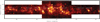 |
Fig. 1 Location of the eight LOSs observed in [N II], RRL, and [C II], indicated + signs, superimposed on a moment 0 integrated intensity map of the Hnα RRL GBT Diffuse Ionized Gas Survey (GDIG; Anderson et al. 2021). None of the LOS intersect the locations of the brightest compact emission, although many intersect larger ionized zones. |
[N II], RRL, and [C II] LOSs.
2.1 SOFIA [N II] observations
The [N II] line at 1461.1338 GHz (λ = 205.178μm) (Brown et al. 1994) was observed using GREAT (Heyminck et al. 2012; Risacher et al. 2016; Durán et al. 2021) onboard SOFIA (Young et al. 2012) as part of the Guest Observer Cycle 7 campaign (proposal ID 07_0009; PI Langer). GREAT was configured with the 4GREAT-HFA (Durán et al. 2021) configuration to observe four lines, [N II] 205 micron, [O I] 63 micron, CO(5–4), and CO(8–7). The observations were made on four flights from June 24 to 27, 2019, from Christchurch, NZ as part of SOFIA’s southern deployment. The [N II] line was observed with the 4G3 pixel of the 4GREAT receiver, and the corresponding half–power beamwidth for the [N II] observations was 19.7" at 1461.1338 GHz. The data were processed with the kosma_ calibrator version 18_06_2019 including atmospheric calibration (Guan et al. 2012). The spectra were calibrated to TA using a forward efficiency of 0.97 and [N II] calibrated to main beam temperature with ηmb = 0.706. First to third order baselines were removed from the delivered data products.
Each ON position observation used an OFF position at the same longitude with b = 0.°4, in order to balance baseline quality with the need to have the OFF position as far above the plane as possible. However, as [C II] and [N II] are widespread throughout the Galaxy, and finding a clean OFF position for proper calibration could be a challenge for observationsof the inner Galaxy. Therefore, every OFF position was checked for [N II] emission by observing each LOS at b = +0.°4 using an OFF position at b = 0.°8. Observations of the Scutum arm in [N II] (Langer et al. 2017) followed a similar approach but also observed secondary and tertiary OFF positions and found that [N II] emission at b ≥ 0.°8 is either absent or relatively weak.
In Fig. 2, we plot [N II] for the LOSs at b = 0.°0, along with the [C II] observations from Herschel HIFI GOT C+ survey (Pineda et al. 2013; Langer et al. 2014). [N II] was detected with high signal-to-noise at five ON positions, with weaker signal-to-noise, at G027.0+0.0, and marginally detected at two velocities for G021.7+0.0, and was not detected at G025.2+0.0. In Appendix A, we plot the [N II] spectra for the first OFF positions at b = 0.°4.
Whenever there was [N II] emission at the b = 0.°4 position we corrected the spectra in the ON position by fitting a Gaussian to the spectrum and adding it to the b = 0.°0 spectrum. Four of the eight LOS had no emission in the OFF position at the level of the rms noise, while three had weak emission, and only G023.5+0.0 had strong emission in the OFF position. Two examples of the before and after correction spectra are shown in Appendix A, one for the strongest source, G023.5+0.0, and one for a typical source, G026.1+0.0. This procedure minimizes the introduction of noise into the target spectra at b = 0.°0. We then refit the baselines for these b = 0.°0 LOS with a third order polynomial setting a window based on the observed emission. The typical rms [N II] noise per 2.0 km s−1 channel is 0.17 K.
2.2 Hydrogen recombination lines
We observed RRLs along all eight LOS in our sample using the Versatile GBT Astronomical Spectrometer (VEGAS) on the GBT in X-band (8 – 10 GHz) in the position switching observing mode. The angular resolution of the GBT in X-band is 84". We used the same lines and procedures as described in Pineda et al. (2019), as follows. For each observed direction, we simultaneously measured seven Hnα RRL transitions, H87α to H93α, using the techniques discussed in Bania et al. (2010); Anderson et al. (2011); Balser et al. (2011), and averaged all spectra together to increase the signal-to-noise ratio using TMBIDL (Bania et al. 2016). All the lines in the band (two polarizations per transition) were averaged together to increase the signal-to-noise ratio and the average frequency is 9.17332 GHz. The GBT data were calibrated using a noise diode fired during data acquisition, and are assumed to be accurate to within 10% (Anderson et al. 2011). The data were later corrected with a third-order polynomial baseline. We converted the intensities from an antenna temperature to main-beam temperatureusing a main beam efficiency of 0.94. The typical rms noise of this data is 2.3 mK when smoothed to a 2 km s−1 channel. The eight RRL lines are plotted in Fig. 2 along with [C II] and [N II].
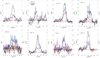 |
Fig. 2 Main beam temperature, Tmb (K) versus velocity for [N II] (red) and [C II] (blue) (right axis and scale) and the corresponding Hnα RRL spectra(black) Tmb (mK) (left axis and scale) for eight LOSs (G020.9+0.0 to G028.7+0.0) at b = 0.°0. [N II] was not detected at G025.2+0.0, and was marginally detected towards G021.7+0.0 at two velocities centered on ~25 and 67 km s−1. |
2.3 GREAT versus PACS 205 μm data
The Herschel Space Observatory open tme key program, Galactic Observations of Terahertz C+ (GOT C+) conducted a sparse survey of velocity resolved [C II] along ~500 LOS throughout the disk (Langer et al. 2010, 2014; Pineda et al. 2013) using the HIFI instrument. Goldsmith et al. (2015) did a follow up survey in [N II] of 149 LOS observed in [C II] by GOT C+. All 149 LOS were observed with Herschel PACS in both fine structure transitions of [N II], 3P2–3P1 at 121.898 μm, with a resolving power of ≃1000 and 3P1–3P0 at 205.178 μm with a resolving power ≃2000. PACS is an array of 25 pixels and its very low spectral resolution provides no velocity information for Galactic LOS, in contrast to the high spectral resolution of HIFI. [N II] was detected in 116 LOS at 205 μm and in 96 of these at 122 μm, where LOS here means the average of the 25 PACS pixels with an effective angular resolution ~47". Details of the PACS data reduction are found in Goldsmith et al. (2015), where it was noted that the 205 μm data had calibration uncertainties due to a red filter leak. With the availability of [N II] from SOFIA GREAT it became possible to calibrate the PACS 205 μm observations.
To compare the PACS intensities with those of the spectrally resolved [N II] data, Pineda (2021, private communication) computed intensities at different angular resolutions by averaging the PACS array pixels weighted with a Gaussian function with FWHM corresponding to the resolution of SOFIA/GREAT and Herschel/HIFI. They compared the weighted intensities of the PACS observations with the ten LOS observed with HIFI (Goldsmith et al. 2015; Langer et al. 2016), seven LOS observed with GREAT (this paper), and one position in the Scutum arm (Langer et al. 2017). The half-power beam width of GREAT at 205 μm is ≃20", while the PACS and HIFI beamwidths are ≃ 15" and 16", respectively. The PACS weighted pixel average at 205 μm is lower by ~30%, on average compared with the HIFI and GREAT spectrally resolved 205 μm intensities. This difference could be due to the different beam sizes, but more likely is a result of the calibration of the PACS 205 μm data affected by the red filter leak (cf. Goldsmith et al. 2015).
In this paper, we have adopted the correction factor suggested by the comparison of PACS with the spectrally resolved data and scaled the PACS 205 μm intensities by 1.3. In Table 2, we list the integrated intensities for seven LOSs observed with GREAT with those of PACS* where PACS* = 1.3 × PACS from Goldsmith et al. (2015). Table 2 lists the LOS, the scaled value of PACS, PACS*, converted to (K km s−1) (see Goldsmith et al. 2015), the integrated [N II] intensity observed with GREAT in (K km s−1), and their ratio. The intensities measured with PACS scaled and GREAT agree reasonably well for the seven positions where [N II] is detected with GREAT. For five of the six LOS I(GREAT)/I(PACS*) ranges from 0.8 to 1.3, which is what we would expect if the spatial distribution across the PACS pixels does not vary much. However, the GREAT intensity for LOS G027.0+0.0 is only about 0.6 that observed by PACS. Along this LOS Pineda (2021, private communication) found that the ratio in the inner 47" of the array is much smaller than the average over the array, which suggests that the emission is non-uniform over the PACS array, and probably explains the difference between the GREAT and PACS intensities. G021.7 is one of the weaker sources in [N II] detected with PACS. We have marginal detections, S/N ~ 3 at two velocities, and here use the total integrated intensity which yields a firmer detection, and has about 74% of the intensity detected with PACS. In the case of G025.2+0.0 we do not detect any [N II] and the 3-σ upper limit is only ~50% of the PACS detection. We have no explanation for the failure to detect [N II] along this LOS, but note that the [C II] is particularly weak which would be consistent with a weak [N II] emission.
Comparing PACS and GREAT 205 μm integrated intensities.
3 Properties of the [N II] and [C II] Gas
In this section, we use the [N II], [C II], and RRL lines to derive the properties of the ionized gas. The RRL antenna temperatures are plotted in milli-Kelvin (left axis) while the main beam temperatures of [C II] and [NII] are plotted in Kelvin (right axis). The RRL emission was clearly detected in seven of the eight LOSs with high signal-to-noise, the exception is G025.2+0.0 where there is a marginal detection at VLSR = 92 km s−1. While all eight LOSs are detected in both [N II] transitions using PACS (Goldsmith et al. 2015), only six are clearly detected in the 205 μm GREAT observations with good S/N. [N II] was marginally detected at G021.7+0.0 and not detected at G025.2+0.0. In contrast, every LOS has detected [C II] emission.
Here, we will use the spectral information combining RRL, [N II], and [C II] emission to derive characteristics of the gas, where possible, such as density, kinetic temperature, turbulent velocity dispersion, column density, and fraction of ionized nitrogen. The analysis of [C II] in particular is complicated by foreground or self-absorption of lower excitation gas containing C+. In principle [N II] spectra may also be affected by foreground absorption, and absorption has been detected in [N II] against continuum sources (Persson et al. 2014). However, the abundance of gas phase nitrogen is typically a factor of 2.5 smaller than carbon (Meijerink & Spaans 2005) and absorption of bright [N II] emission is likely to be less important. We see no clear evidence of absorption in our [N II] data. In contrast to H+ and N+ which are confined to highly ionized gas, C+ is widespread throughout the Milky Way and can be found in many low density, and hence low excitation foreground environments which are capable of absorbing high excitation [C II] emission. For example, [N II] and [C II] are comparable in intensity forseveral LOSs, and [N II] is even brighter than [C II] in G028.7+0.0 peaking at a local minimum in [C II]. Similar behavior was seen in other LOS where [C II] and [N II] were spectrally resolved (Goldsmith et al. 2015; Langer et al. 2016) and possibly result from foreground absorption.
3.1 Kinetic temperature and velocity dispersion
The kinetic temperature of the ionized gas is a critical parameter in calculating the properties of the gas as the collisional de-excitation rate coefficients for the fine structure levels of [N II] are temperature dependent (Tayal 2011), as are those of [C II] (Tayal 2008). The temperature is also an important constraint for modeling the heating and cooling of the gas, distinguishing whether collisional ionization is important or not. Finally, the temperature and density determine the thermal pressure of the gas and factor into whether the gas is thermally confined or will dissipate and on what time scale.
In their derivation of n(e) and N(N+) Goldsmith et al. (2015) adopted a fixed canonical temperature, 8000 K, characteristic of warm ionized gas. Whereas Pineda et al. (2019) used a fit to the temperature as a function of galactocentric distance derived from the ratio of the hydrogen RRL line-to-continuum emission measurements in H II regions (e.g., Balser et al. 2015), which is independent of n(e) and proportional to  . Balser et al. (2015) derived electron temperatures for a large sample of H II regions across the Galaxy and find that they range from ~4500 K to ~13 000 K with a fit, Te = 4446 + 467Rgal (kpc). The [N II] emission studied here are all located in a rather narrow range of Galactic longitude, ~20° to 30°, corresponding to Rgal ~ 4–6 kpc, which would imply a characteristic temperature ~6300–7300 K, using the results in Balser et al. (2015). However, the temperature gradient derived by Balser et al. (2015) may not apply to the D-WIM regions studied here, which have much lower electron densities than H II regions and therefore may have different characteristic temperatures.
There are a number of other techniques to derive the kinetic temperature of the gas. One is from excitation analysis of two or more levels which have different excitation energies comparable to, or larger than, the kinetic temperature. However, this approach does not work in the hot highly ionized gas as the two fine structure lines of [N II] arise from levels with excitation energies ~70 and 188 K above the ground state. These are much lower than the kinetic temperature and so the intensities of these lines are insensitive to temperature in ionized regions with temperatures greater than several hundred Kelvin. Another approach is to compare line widths of species with different mass that emit from the same volume, where the larger the mass contrast the larger the difference in thermal linewidth and thus more readily to determine the thermal temperature.
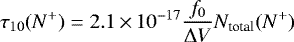
Here we take advantage of the factor of 14 difference in mass of N+ and H+ and their different line widths ΔV (RRL) and ΔV [N II], to derive the thermal and turbulent line widths, and then the thermal temperature. In using these line widths to derive the thermal andturbulent velocity dispersion, we neglect the contribution of velocity gradients, opacity, and pressure broadening. The [N II] opacity at the peak is adapted from Langer et al. (2016),
 (1)
(1)
where ΔV is in km s−1, and f0 is the fractional population in the ground state. For a column density N(N+) = 2 × 1017 cm−2 (see Table 2 Goldsmith et al. 2015), Tth = 8000 K, ΔV = 10km s−1, and f0 ≥ 0.5, typical for n(e) = 10–35 cm−3, the opacity τ < 0.25, and opacity broadening can be neglected (a similar result is shown in Fig. 15 in Goldsmith et al. 2015).
We cannot rule out line broadening due to systematic motions as we do not have maps in [N II] with which to determine the velocity field. We believe that pressure broadening is not likely to be important because there is little evidence of non-Gaussian line shapes for strong lines, in addition a calculation of pressure broadening in a fully ionized hydrogen plasma is beyond the scope of this paper. A further uncertainty is that the beam widths of the RRL and [N II] observations are quite different, which could alter the line shape for non-uniform regions. In the PACS observations, at many LOSs, the [N II] emission is roughly constant across the ~48" × 48" array (~1 pc2 at a distance of ~4 kpc), whereas for other LOS it is non-uniform (Goldsmith et al. 2015). This difference can be seen in Fig. 7 of Goldsmith et al. (2015) which compares the HIFI observations to PACS with different pixel averaging. Here we assume that the different RRL and [N II] beamsizes do not significantly affect the line shape, which is less prone to error than the peak intensities. The largest uncertainty, in our view, is the fitting of [N II] lines with multiply blended components, as seen in G023.5+0.0 and in several LOS in Langer et al. (2016).
The solutions are derived in Appendix B and for N+ and H+ are given by,
![Mathematical equation: \begin{equation*}\Delta V_{\textrm{th}}(\textrm{H}^+) = \bigg (\frac{M_{\textrm{N}}}{M_{\textrm{N}}-M_{\textrm{H}}}\bigg)^{0.5}[\Delta V_{\textrm{obs}}^2(H^+)-\Delta V_{\textrm{obs}}^2(\textrm{N}^+)]^{0.5}\, ${km\,s$^{-1}$}$\end{equation*}](/articles/aa/full_html/2021/07/aa40223-20/aa40223-20-eq9.png) (2)km s−1
(2)km s−1
 (3)km s−1
where, ΔVobs, ΔVth, and ΔVturb are the observed, thermal, and turbulent Full Width Half Maximum (FWHM) line widths, respectively, and MH and MN are the hydrogen and nitrogen atomic mass, respectively. In the positions without detection of [N II] we can place a strict upper limit on the thermal temperatures from the width of the hydrogen RRL lines.
We fit a Gaussian to the RRL and [N II] lines to derive ΔV which is the Full Width at Half Maximum, FWHM. In some LOS the RRL and [N II] lines have a single peak and similar line shape consistent with only one component. Other LOS spectra show structure that is suggestive of two (or more) components, and we have fit these with two Gaussians. In the case of [N II] the number of components we can fit is limited by the noise level to one or two Gaussians. In Table 3, we list the Gaussian fits to the RRL and [N II] spectra along with the 1-σ rms error where Tp is the peak temperature, Vp the velocity of the Gaussian peak, and ΔV, the full width half maximum of the Gaussian.
In Table 4, we list the upper bound on the H+ temperature, Tupper(H+) derived from the RRL Gaussian fits solution to ΔVobs and Eq. (B.3). We derive, where possible, the thermal and turbulent linewidths using Eqs. (2) and (3), and the thermal temperature of H+. The H+ thermal temperatures derived from [N II] and RRLs lie in the range 3200–8500 K. The two main sources of error for the derived physical parameters are the intensity of the 205 μm emission (that of the 122 μm line is much smaller (see Table 2 Goldsmith et al. 2015) and the temperature, Tth because of the dependence of the electron collisional rate coefficients on the population of the [N II] levels (see Fig. 3). We also list the 1-σ rms errors for the solutions. There is no solution for the one LOS without detectable [N II] emission, G025.2+0.0. We also list the thermal and turbulent linewidths, which are typically the same order of magnitude in H+, but for N+ the broadening is dominated by turbulence.
Spectral line Gaussian parameters.
3.2 Electron density and N+ column densities
In the optically thin limit, which likely applies to [N II] (Goldsmith et al. 2015), we can solve exactly for the electron density, n(e), and N+ column density, N(N+), given the temperature of the ionized gas, and the intensities of the 122 and 205 μm lines. Goldsmith et al. (2015) adopted a fixed kinetic temperature of 8000K as typical of the temperature of the ionized gas, whereas we use the kinetic temperatures derived from the line widths in the five LOS observed in [N II] 205 μm.
There was not, nor currently is there, a capability to observe a spectrally resolved 122 μm line. Therefore, to calculate the electron density from the ratio of the 122–205 μm lines we use the PACS data from Goldsmith et al. (2015), but the 205 μm data will be scaled by 1.3 to account for the revised calibration discussed in Sect. 2.3.
The electron density can be obtained from the ratio of the 122 and 205 μm intensities, and in intensity units of W m−2 sr−1, we have (Eq. (19) in Goldsmith et al. 2015),
 (4)
(4)
where fi is the fractional population of level i (as defined in Eq. (6) of Goldsmith et al. 2015) and I is in units of W m−2 sr−1. In Fig. 3, we plot I122∕I205 as a function of n(e) for temperatures from 2000 K to 20 000 K, corresponding to the range of temperatures appropriate to the ionized gas. It can be seen that the values ofn(e) are sensitive to the kinetic temperature to about 20% at the low end of the density range, n(e) ~ 10 cm−3, and about 50% at the high end, n(e) ~35 cm−3 over the range considered here. This sensitivity is not due to the excitation energy of the fine-structure levels, which are negligible compared to the kinetic temperature, but to the temperature dependence of the collisional de-excitation rate coefficients (Tayal 2011). We derived values of n(e) for the six LOS with [N II] 205 μm detections with GREAT at high S/N using these temperature sensitive equations and they are listed in Table 5 along with the distance from the Galactic center, Rgal in kpc, calculated following the approach in Pineda et al. (2019, see Sect. 3.2), and the kinetic temperature. The electron densities we derived using the Tkin (K) determined in this paper are generally smaller by 50% than the values derived by Goldsmith et al. (2015) with a fixed Tkin (K) = 8000 K. The contributions to this reduction are the use of the calibration update described above which increases the PACS 205 μm intensity, and to generally lower temperatures derived for each region, which change the collisional de-excitation rate coefficients, as seen in Fig. 3.
The column density of N+ can be calculated from the intensity of the 205 μm line given Tkin (K) and n(e). We use the GREAT [N II] spectra to calculate the column densities, except for G025.2+0.0 where we do not have a detection and G021.7 where the detection is marginal. In the optically thin limit the column density of N(+) is given by,
 (5)
(5)
where f1 is the fractional population of the 3P1 level (Eq. (6) in Goldsmith et al. 2015) and the values of N([N II]) are given inTable 5 along with those from Table 2 in Goldsmith et al. (2015). The ratio of the column densities from both calculations vary considerably with NGREAT([N II])/NPACS([N II]) ranging from 0.5 to 2, which reflects the differences in calibration, electron density, and kinetic temperature. In Table 5, we also list the average size of the [N II] emission region defined as,
 (6)
(6)
In the following sections, we derive the hydrogen ion column density and, assuming N+ and H+ occupy the same volume, the fractional abundance of N+, x(N+).
Ionized gas parameters.
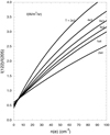 |
Fig. 3 Intensity ratio of the 122–205 μm lines in W m−2 sr−1, versus electron density for kinetic temperatures Tkin (K) ranging from 2000 K to 20 000 K. The curves are labeled by Tkin (K) and employ the collisional de-excitation rate coefficients of Tayal (2011). |
Electron densities and N+ column densities.
H+ column densities and N+ fractional abundance.
3.3 H+ and N+ column densities
The H+ column densities, N(H+), were derivedfrom the RRL lines using the approach described in Pineda et al. (2019) and are listed in Table 6, along with N(N+) from our analysis of the GREAT data. Also listed in Table 6 are the distance from the Galactic center, Rgal, electron density, n(e), kinetic temperature, Tkin, the integrated intensity of the [N II] observed with GREAT used to derive N(N+). From N(N+) and N(H+) we derive the fractional abundance of nitrogen ions, x(N+) and these are listed in Table 6. For reference we also list the solutions for n(e) and N(N+) derived by Goldsmith et al. (2015) using the PACS pixel averaged intensities of the 122 and 205 μm lines.
3.4 Fractional abundance of N+
The fractional abundances of metals as a function of Galactic radius are important parameters for understanding the baryonic lifecycle of the Galaxy. The nitrogen abundance distribution depends on the star formation history of the Galaxy because it is produced by primary and secondary nucleosynthesis in intermediate and massive stars (Johnson 2019). Optical observations have traditionally been used to trace metallicity in the solar neighborhood, but extinction by grains makes this approach more difficult to probe the inner Galaxy. The infrared observations of [C II], [N II], and [O I] are useful probes of the metallicity because they are not readily absorbed by dust and can probe the inner Galaxy where much of star formation takes place.
Using the derived column densities of N+ and H+ we can evaluate the fractional abundance of nitrogen in the singly ionized state. In Table 6 we list the fractional abundances x(N+) for all LOSs where we have detected [N II] and RRL lines and plot them as a function of Rgal in Fig. 4. The fractional abundance of N+ ranges from 1 to 3 × 10⁻⁴, which implies an enhanced nitrogen abundance at a Galactic radius about 4.3 kpc, which is an average distance for the [N II] emission, and corresponds to the inner edge of the Milky Way’s molecular ring.
The average value of x(N+) ~ 1.9 × 10⁻⁴ at Rgal ≃ 4.3 kpc is about 2.6 times the nitrogen abundance in the local ISM, ~7.2 × 10⁻⁵ (Meijerink & Spaans 2005), indicating significant enhancement in metallicity in the inner Galaxy. Pineda et al. (2019) analyzed the nitrogenabundance in the ten LOSs observed with HIFI in the Goldsmith et al. (2015) survey, using RRLs to derive N(H+). The HIFI data cover a much wider range in Rgal, 0–13 kpc, which made it possible to derive an abundance gradient, 12 + log(N+/H+) = 8.40–0.076Rgal. In the HIFIdata (in Table 3 Pineda et al. 2019) there are four data points at ~4.4 kpc, whose average fractional abundance is 1.4 × 10⁻⁴, about 25% lower than the value derived here.
All the conclusions about the abundance of nitrogen, whether derived from visual or far-infrared observations, assume that nitrogen is entirely in the singly ionized state. However, as discussed in Sect. 4, this depends on the density and temperature of the ionized gas, and the intensity of the extreme UV (EUV) field (photon energies > 13.6 eV) which regulate the ionization distribution (Langer et al. 2015). If nitrogen is in neutral (N) or highly ionized states (mainly N2+) then the x(N+) values calculated here and in Pineda et al. (2019) are only lower limits. Indeed there is evidence for doubly ionized nitrogen from observations of [N III] at 57 μm in diffuse regions of Carina (Mizutani et al. 2002), which could be associated with the D-WIM. The presence of N2+ and higher ionization states would result in an underestimate of the fractional abundance of nitrogen. However, without observationsof [N III] along the LOSs studied here, we cannot say whether this effect is important here.
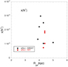 |
Fig. 4 Fractional abundance of N+, x(N+), derived from [N II] and the RRL emission lines. The values derived from GREAT are shown in black, while those from HIFI (in Table 3 Pineda et al. 2019) that are at the same Galactic latitude are plotted in red. |
[C II] emission fraction from highly ionized gas.
3.5 [C II] Emission from highly ionized gas
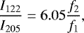
In principle, the [N II] emission can be used to determine how much [C II] arises from highly and weakly ionized gas because, as discussed above, [N II] exists only in highly ionized gas such as the D-WIM, WIM, or H II regions. It can be shown that over a wide range of electron densities that the [N II] intensity predicts how much [C II] should arise from the highly ionized gas as discussed for the Milky Way (e.g., Goldsmith et al. 2015; Langer et al. 2016) and in extragalactic sources (e.g., Croxall et al. 2017). For effectively optically thin emission the intensity of [C II] for ionized gas, Iion ([C II]) is given by Eq. (4) in Langer et al. (2016),
![Mathematical equation: \begin{equation*}I_{\textrm{ion}}(\textrm{[CII]})=0.675\frac{f_{3/2}}{f_1}\frac{x({\textrm{C}^+})}{x({\textrm{N}^+})}\ I_{\textrm{ion}}(\textrm{[NII]})\,\, {(\textrm{K\, km\,s}^{-1})}\,\,\end{equation*}](/articles/aa/full_html/2021/07/aa40223-20/aa40223-20-eq14.png) (7)
(7)
where f3∕2 and f1 are the fractional populations of the 2P3∕2 and 3P1 levels of C+ and N+, respectively, and x(C+) and x(N+) are the fractional abundances of carbon and nitrogen ions. In Fig. 5, we plot the ratio of the population of the levels f3∕2 (C+) to f1 (N+) as a function of electron density for electron temperatures in the range 2,000 to 10 000 K, which are most appropriate for the regions observed in Hnα RRL and [N II]. The ratio uses the collisional rate coefficients for electrons given by Tayal (2008, 2011), and the Einstein Aul are from Schöier et al. (2005). The ratio f3∕2 (C+) to f1 (N+) is remarkably insensitive to electron density and temperature over the range shown in Fig. 5.
We calculate Iion([C II]) in Eq. (6) using the values of n(e) given in Table 7. Here, for simplicity, we assume that all the carbon and nitrogen are in singly ionized states so x(C+)/x(N+) is just the elemental carbon to nitrogen ratio (which may not be valid in the presence of a strong EUV flux). The gas phase abundances of carbon and nitrogen in the inner Galaxy are larger than that in the solar neighborhood (Rolleston et al. 2000; Esteban & García-Rojas 2018). In the solar neighborhood, x(C) ≈ 1.4 × 10⁻⁴ and x(N) ≈ 5.2 × 10⁻⁵, yields a x(C/N) ratio of 2.7. Esteban & García-Rojas (2018) find a nitrogen Galactic radial gradient, log(N/H) = −3.79−0.059Rgal, for Rgal > 6 kpc, where RG is in kpc. Their results are based onoptical observations and so cannot directly probe the inner Galaxy. Extrapolating their relationship to the average radius for [N II] emission, RG ≈ 4.3 kpc, yields x(N) ≈ 9.0 × 10⁻⁵. For carbon, Rolleston et al. (2000) derived a fractional abundance relationship as a function of Galactic radius, which has been rewritten by Pineda et al. (2013) as x(C+) = 5.5 × 10−410−0.07RG, and has a value of 2.7 × 10⁻⁴ at 4.3 kpc, giving a ratio x(C/N) = 3.0, close to the value of 2.9 adopted by Goldsmith et al. (2015). Instead of the extrapolation of the optical results to the inner Galaxy we also have the study of [N II] and RRL in the inner Galaxy by Pineda et al. (2019) who derived a slightly different slope from measurements of Rgal = 0–13.2 kpc. They found that log(N/H) = −3.6–0.076Rgal, which gives x(N) = 1.1 × 10⁻⁴ at Rgal = 4.5 kpc, about 30% higher than the Esteban & García-Rojas (2018) value. Combining the N+ results from Pineda et al. (2019) and C+ from Rolleston et al. (2000) yields a carbon to nitrogen ratio, x(C/N) = 2.33, about 20% smaller than the value based on Esteban & García-Rojas (2018) and adopted by Goldsmith et al. (2015). Here we adopt the lower value for the C+ to N+ ratio using the results of Pineda et al. (2019) combined with Rolleston et al. (2000) which yields a more conservative estimate of the [C II] emission predicted to arise from the highly ionized gas using Eq. (7).
In Table 7 for each LOS we list the observed line intensities, Itot ([C II]) and Itot ([N II]) in K km s−1, the calculated [C II] ion intensity, Iion([C II]) using Eq. (7), and the fraction of [C II] emission arising from the ionized and neutral gas. The ratio of f3∕2/f1 used in Eq. (7) is calculated using the values of n(e) and Tkin(e) derived here (Tables 5 and 6, respectively), although as shown in Fig. 5 this ratio is not sensitive to either parameter.
For five of the six LOS in which [N II] was detected, the intensity of [C II] in the highly ionized gas traced by [N II] is a significant source of [C II], representing 50% to 80% of the total observed [C II] in these LOS. In one LOS, G028.7+0.0, the estimated [C II] emission from the ionized gas is greater than the observed [C II] intensity. This result is similar to what has been seen in other LOS in which [N II] has been detected (Goldsmith et al. 2015; Langer et al. 2016; Croxall et al. 2017). The fact that the predicted [C II] from the highly ionized region is large suggests that a significant fraction of the observed [C II] comes from the highly ionized dense ionized warm interstellar medium (D-WIM). This result is significant because it indicates that the dense WIM emits [C II] comparable to that from PDRs and CO-dark H2 clouds.
In G028.7+0.0, the predicted [C II] from the ionized gas is greater than the observed [C II] and this deficiency in [C II] emission is likely due to foreground absorption at ~103 km s−1 where [N II] peaks, but [C II] shows a clear local minimum. Foreground absorption of [C II] is seen in other LOS (Langer et al. 2016, 2017) and so appears to be a common feature of the [C II] emission. There is also evidence from [13 C II] detections that [C II] has moderate to high opacity in bright [C II] sources (Guevara et al. 2020; Kirsanova et al. 2020). Evidence of deep foreground absorption was established by Graf et al. (2012) from observations of [C II] and [13 C II] providing direct evidence of large column densities of cold foreground [C II] capable of absorbing background [C II]. However, whether absorption of [C II] can explain all of the emission deficiency or not, the very large fraction of [C II] that appears to arise from the highly ionized gas suggests that a significant fraction of Galactic [C II] emission is absorbed by lower excitation foreground gas.
There is one other potential effect on using [N II] to calculate the contribution of highly ionized gas to the [C II] budget, namely the possibility that the EUV field, or X-rays, produces doubly ionized nitrogen, N2+, or even higher ionization states, as seen in the detection of [N III] towards highly ionized regions (e.g., Mizutani et al. 2002) and in H II – PDR models (Abel et al. 2005; Kaufman et al. 2006). We discussed the effect of having highly ionized nitrogen on modifying results that measure the fractional abundance of nitrogen in Sect. 3.3. However, the effect of EUV and/or X-rays producing multiply ionized states is less important in calculating the ratio of C+ to N+ because these ionization processes produce both multiply ionized nitrogen and carbon (Langer & Pineda 2015), thus preserving, to first order, the carbon to nitrogen ratio derived from C+ and N+.
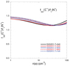 |
Fig. 5 Ratio of the population of the levels f3∕2(C+) to f1 (N+) as a function of electron density for kinetic temperatures in the range 2000–10 000 K. |
4 Discussion
The dense WIM (D-WIM) represents a newly identified state of the ISM with properties different from those of other highly ionized components of the ISM. For example, the temperatures we derived for the dense warm ionized gas range from 3400 K to 8500 K, comparable to the temperatures derived for dense H II regions and the low density WIM. Whereas the D-WIM electron densities are much larger than those of the WIM and much lower than in H II regions. We do not yet know the role of the D-WIM in the lifecycle of the ISM, for example, how it forms and evolves. Here we outline some properties of the D-WIM and discuss the likely ionization process sustaining N+.
4.1 Dense ionized gas component in the ISM
The [N II] emission presented here and in the survey by Goldsmith et al. (2015) primarily trace dense ionized gas rather than the WIM which has a density too low to produce the observed intensities. Furthermore, the widespread distribution seen in the PACS survey indicates that the D-WIM is a distinct component of the interstellar medium associated with [C II] emission. All the [N II] detections are associated with CO emission, as can be seen in Fig. 6 which compares the [N II] spectra towards the six LOS with the 12CO(J = 1−0) spectra from the GOT C+ survey (Pineda et al. 2013; Langer et al. 2014). However, not all the CO detections have [N II] emission characteristic of the D-WIM. In addition, in most cases where [N II] and 12CO are detected there is a velocity shift of [N II] with respect to CO, which might indicate a dynamical evolution, although we cannot rule out that some of it could be the result of CO absorption.
We can also see in the GDIGS maps (Fig. 1) that the [N II] LOS do not intercept the brightest emission, probably characteristic of compact H II sources, but rather are primarily located at the edges of the Hnα emission. The velocity shift between [N II] and CO is consistent with the D-WIM being associated with star-forming regions which are themselves associated with molecular gas clouds. This shift indicates that the D-WIM gas traced by [N II] is likely undergoing dynamical evolution, probably a result of energy input from nearby H II regions seen in the GDIGS survey shown in Fig. 1. However, without maps of [N II] we cannot describe the dynamics of the ionized gas. What is clear is that, unlike the widespread WIM which fills large volumes of the ISM, the D-WIM likely occupies a relatively narrow layer associated with star-forming regions.
The D-WIM could be a density enhancement in the WIM, as pulsar dispersion measurements suggest that the WIM is clumpy (see review by Haffner et al. 2009). However, the [N II] spectra presented here are associated in velocity space with [C II] and CO, so it seems unlikely that the D-WIM is associated with dense clumps in the WIM.
Another aspect of the D-WIM is that its thermal pressure P = n(e)Tkin(H+) ranges from ~3 × 10⁴ to 2 × 10⁵ (K cm−3), which is much higher than that of the traditional low density WIM, P ~ 800 (K cm−3) assuming a WIM uniform electron density, n(e) ~ 0.1 cm−3 and temperature, Tkin ~ 8000 K. At these pressures the D-WIM would dissipate rapidly unless it was either formed continuously or gravitationally bound to a molecular cloud. The expansion would take place on a time scale of the size of the D-WIM layer divided by the sound speed of hydrogen. From Table 5, the size of the N+ layer, ⟨ L⟩ (N+) = N(N+)/n(e), ~ 1011 km and the sound speed is ~5–10 km s−1, yielding a dissipation time ~300 yr.
4.2 Ionization of nitrogen
The presence of dense ionized nitrogen bears on the ionizing environment as only three processes are important in converting N → N+; these are electron collisional ionization, proton charge transfer, and extreme ultraviolet (EUV) photoionization. In the absence of EUV the first two processes are temperature sensitive but the fractional abundance of N+ is essentially independentof electron density as electron recombination is the dominant loss mechanism in a fully ionized gas (unless the temperature is so high that N+ can be collisionally ionized to N2+). If EUV photoionization dominates the production of N+ then the fractional abundance is sensitive to the electron density through the recombination mechanism. Thus, knowledge of the density and temperature of the dense ionized gas is essential to understand the formation and destruction of nitrogen ions. Furthermore, the hardness of the EUV, its intensity as a function of wavelength will determine whether higher ionization states exist due to photoionization of N+ → N2+.
Geyer & Walker (2018) addressed the ionization of the D-WIM based solely on electron collisional ionization of N and found that they required a kinetic temperature of ~19 000 K to explain the presence of dense ionized gas as given by the PACS results (Goldsmith et al. 2015). A high kinetic temperature is necessary for collisional ionization due to the large ionization potential for e + N → N+ + 2e of 14.534 eV. The kinetic temperatures we derive are clearly in conflict with their conclusions. However, we note that they neglected to include proton charge exchange and EUV photoionization of nitrogen as possible production of N+. We have previously discussed electron collisional and proton charge exchange ionization of nitrogen and its sensitivity to the temperature of the gas (Langer et al. 2015). Below we consider each of these processes separately to understand the likely source of nitrogen ionization in the D-WIM.
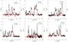 |
Fig. 6 Main beam temperature, Tmb (K), versus velocity for [N II] spectra (red) and 12CO(1–0) (black) for the six LOS where [N II] was clearly detected. |
4.2.1 Collisional ionization of nitrogen
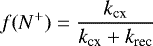
If we consider that the only processes controlling the ionization balance of nitrogen are electron collisional ionization, e + N → N+ + 2e, and electronic recombination (electronic + di-electronic), N+ + e → N + hν, then we have for the fractional abundance f(N+),
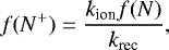 (8)
(8)
independent of the electron abundance and only dependent on the temperature through the reaction rate coefficients for ionization, kion, and electron recombination, krec. Substituting for the conservation of nitrogen, f(N+) + f(N) = 1, we have
 (9)
(9)
The reaction rate coefficients for electron collisional ionization are derived from thermally averaged cross-sections and we use the fits derived by Voronov (1997). The recombination rate coefficients for nitrogen are from Nahar & Pradhan (1997). In Fig. 7, we plot the solutions for electron collisional ionization of nitrogen in terms of f(N+) as a function of kinetic temperature of the plasma, Tkin (K), for temperatures up to 3 × 10⁴ K. We neglect ionization to higher ion states because the effect is unimportant due to the high ionization potential for N+ → N2+ of 29.6 eV. As can be seen in this figure electron collisional ionization is negligible below 104 K, and it requires a temperature > 1.6 × 10⁴ K for nitrogen to be 50% ionized, and over 2.5 × 10⁴ for nitrogen to be essentially fully ionized.
Proton charge exchange ionization of nitrogen, p + N → N+ + H, is more important than electron collisional ionization at low temperatures because the ionization barrier is the difference in ionization potential between H+ (13.598 eV) and N (14.534 eV), ΔIP = 0.936 eV, or in units of Kelvins, 1.09 × 10⁴ K. If the only important collisional processes are proton charge exchange and electron collisional ionization, then we can solve for f(N+) in a similar approach to Eq. (9), but replacing kion with the charge exchange collisional reaction rate coefficient, kcx,
 (10)
(10)
where we use the fits to kcx (N+ + H → N + H+) as a function of Tkin given by Kingdon & Ferland (1996) multiplied by exp(-ΔIP/Tkin) to solve for the H+ + N rate coefficients. In Fig. 7, we plot the fractional abundance, f(N+), when only proton exchange and electron recombination are important (red line). It can be seen that proton charge exchange is much more effective than electron collisional ionization in producing N+ and begins to ionize the nitrogen measurably above 5000 K. By 104 K the nitrogen is about 40% ionized, but reaches a maximum of about 50% at 16 000 K. We also plot f(N+) when both electrons and proton reactions are considered (black curve), showing how the combined processes keep nitrogen partially ionized above 104 K, but still require temperatures of order 20 000 K to reach a nearly fully ionized state. In order to sustain nearly fully ionized nitrogen in the H+ plasma at the temperatures we measured in [N II], Tkin ≤ 104 K, requires EUV photoionization.
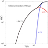 |
Fig. 7 Fractional abundance of ionized nitrogen, f(N+), when the only operative processes are electron collisional ionization and recombination (blue) as a function of the plasma temperature, Tkin (K), compared to f(N+) when the only collisional processes are proton charge exchange and recombination (red). In a realistic case both processes occur simultaneously and the corresponding behavior for f(N+) is plotted asthe black curve. |
4.2.2 Photoionization of nitrogen
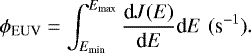
Here we explore how EUV photons can keep nitrogen ionized in the D-WIM regions with moderate electron densities. Young hot stars are sources of ultraviolet radiation that impact the interstellar environment by ionizing atoms and molecules, dissociating molecules, and heating the dust and gas. The ionization potentials for carbon and nitrogen are 11.2603 and 14.5341 eV, respectively. Thus, carbon is readily photoionized by far-ultraviolet photons (λ > 912 Å) while nitrogen photoionization requires extreme ultraviolet photons (λ < 912 Å). The EUV radiation produces highly ionized gas that manifests itself as a surrounding or nearby H II region. Furthermore, the EUV from bright H II sources can leak through holes or clumpy regions of PDRs and sustain a highly ionized gas (Anderson et al. 2015; Luisi et al. 2016). The photoionization rate of nitrogen by the EUV field is
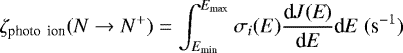 (11)
(11)
where dJ(E)∕dE is the EUVspectral energy distribution in units of photons cm−2 s−1 eV−1, σ(E) is the photoionization cross sectionin cm2, and Emim and Emax are the minimum and maximum energies, respectively, in eV.
Whereas the EUV flux from a cluster of massive stars decreases with energy (Abel et al. 2005; Kaufman et al. 2006), the cross section for photoionization of nitrogen is relatively flat from threshold to ~25 eV (Samson & Angel 1990) except for several very narrow resonances. In addition, the flux of EUV photons decreases with energy and at 20 eV is roughly a third of that at the Lyman limit at 13.6 eV (Abel et al. 2005; Kaufman et al. 2006; Sternberg et al. 2003), decreasing to about 10% at 25 eV. Thus, if we restrict the integral to Emin = 14.534 to 20 eV, to a good approximation, we can take σ(E) to be constant σ0 ≃ 1.1 × 10⁻¹⁷ cm2, and
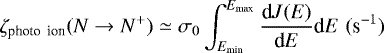 (12)
(12)
where term in the integral is just the EUV photon flux between Emin and Emax,
 (13)
(13)
Thus the nitrogen ionization rate is given by,
 (14)
(14)
More sophisticated approaches can be found in the models of the H II to PDR transition (Abel et al. 2005; Abel 2006; Kaufman et al. 2006).
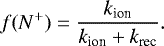
Using these approximations in the balance equation for photoionization of nitrogen and electron recombination of N+, and neglecting other processes yields a fractional ionization,
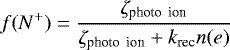 (15)
(15)
and the solution depends on both electron density, n(e), and temperature, Tkin (K). To have nearly fully ionized nitrogen we need ζphoto ion > 5 × krecn(e), or  4.5 × 10¹⁷krecn(e).
In Fig. 8, we plot ϕEUVmin (photons cm−2 s−1) as a function of temperature for n(e) = 10 cm−3, a representative lower limit on density for the D-WIM, such that the lower bound for the EUV photon flux can easily be scaled to other densities. To have a highly ionized nitrogen plasma requires an EUV photon flux ≳ a few × 106 photons cm−2 s−1 at n(e) = 10 cm−3 and scales with density. EUV fluxes of this order are associated with massive star-forming regions (Sternberg et al. 2003; Abel et al. 2005; Kaufman et al. 2006).
4.3 [C II]Emission from the D-WIM
The question of the origin of [C II] underlies an important and longstanding quest to understand the composition of the interstellar medium, how [C II] emission influences it via cooling the gas, how its emission is affected by star formation heating and ionizing the ISM, and how reliable [C II] emission is as a measure of the star formation rate in galaxies. H I 21-cm, CO mm and submm rotational lines, and the C+ far-infrared (FIR) fine structure line, [C II], are among the most important gas tracers that reveal the structure, dynamics, and evolution of galaxies. Whereas the CO is confined to the shielded regions of molecular clouds and N+ only in highly ionized gas, C+ is found in many of the phases of the ISM in both weakly and highly ionized regions. The weakly ionized phases are diffuse H I clouds, diffuse molecular clouds without CO, the so called CO-dark H2 clouds, and PDRs bounding dense molecular clouds. The highly ionized phases with [C II] emission are the WIM, with low electron densities, n(e) ≲ 0.1 cm−3, and high temperatures, Tkin ~ 8000 K, dense H II regions, the Dense WIM (D-WIM), and X-ray dominated regions (XDRs). Disentangling the [C II] contribution from different phases of the ISM is an important goal given the critical importance of [C II] in studying Galactic structure, and the star formation rate.
Carbon, with its ionization potential of 11.26 eV, is readily ionized by far-ultraviolet (FUV) radiation (λ < 912Å) that is pervasive throughout the ISM. Therefore, C+ can be found in weakly and highly ionized gas. In contrast, atomic nitrogen with an ionization potential of 14.5 eV only exists in highly ionized gas that is bathed in extreme ultraviolet (EUV) or X-rays, or is in a hot enough plasma where collisional ionization and proton charge exchange can keep it ionized (Langer et al. 2015, 2016; Langer & Pineda 2015). In Sect. 3.5, we showed that the [N II] emission implies that the D-WIM gas emits a significant fraction of the total [C II] along the observed LOSs. This result is consistent with prior studies of Galactic and extragalactic [N II] and [C II] (Goldsmith et al. 2015; Langer et al. 2016; Croxall et al. 2017).
The conclusions regarding the [C II] emission from the D-WIM rest on a number of assumptions, as discussed in Sect. 3.5, such as the local gas phase nitrogen to carbon abundance ratio, and the foreground opacity, but less so on temperature and density over the range of conditions derived for the D-WIM. In fact, as discussed in Sect. 3.5 there is clear evidence for foreground absorption of [C II] (Langer et al. 2016) taken as part of the PACS [N II] survey (Goldsmith et al. 2015), and in the SOFIA GREAT Scutum arm observations (Langer et al. 2016). In contrast, there is little or no evidence of foreground absorption of [N II] in the HIFI or GREAT data, and using Eq. (1) we estimate that the foreground WIM has an opacity in [N II] ≲0.1. However, unlike [N II], [C II] is also absorbed by the low density diffuse atomic and molecular clouds. An estimate of the degree of absorption was obtained by Langer et al. (2016) who reconstructed the likely [C II] intensity before absorption by fitting the line wings and shoulders of some [C II] lines. He found that the reconstructed [C II] spectra intensity increased by ~50% to 75%. Thus, as the [C II] LOS observed with SOFIA GREAT do not appear to have large opacities or be significantly absorbed, within a factor of two, and are associated with molecular CO gas (Pineda et al. 2013; Langer et al. 2014), it implies that the [N II] regions contribute a significant fraction of the observed [C II].
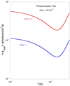 |
Fig. 8 EUV photon flux required to maintain an ionized fraction of 50%, N+/N = 1, (blue curve) and 83%, N+/N = 5, (red curve) for a density of n(e) = 10 cm−3, when the only loss processes is electron recombination as a function of the plasma temperature, Tkin (K). The curves are proportional to density. |
5 Summary
The dense WIM is a recent addition to the known highly ionized interstellar medium components (e.g., WIM, H II, hot ionized medium (HIM)). The N+ fine structure lines at 205 and 122 μm are important probes of the D-WIM as, in contrast to [C II], they arise only in highly ionized gas due to having an ionization potential above the Lyman limit. The nature and origins of the D-WIM are unclear. We do not yet understand how it formed, is heated, and can survive against its thermal pressure. Nor is it clear why it is more prominent in the inner Galaxy (− 60° ≤ l ≤ 60°), and what is its actual contribution to the [C II] Galactic emission. In this paper we have attempted to shed more light on the D-WIM by characterizing its temperature, electron density, N+ column density, and fractional abundance with respect to the H+ column density. We have done so by observing spectrally resolved [N II] 205 μm emission with SOFIA GREAT towards eight LOS in the inner Galaxy (l ~ 20° to 30°) along with hydrogen RRLs observed with the GBT.
We detected eight [N II] components in six of the eight LOS observed and all are associated with [C II] emission, however not all [C II] components have [N II] features. In addition, we had two marginal detections along G027.1+0.0, both aligned with [C II]. It is important to evaluate the role of [N II] in producing [C II] throughout the Galaxy for interpreting the use of [C II] and [N II] as tracers of the ISM and the baryonic lifecycle. The PACS survey found a very high correlation between [C II] and [N II] detections, > 95% of 70 LOS, in the inner Galaxy (−30° to +30°), but a weaker correlation in the outer Galaxy. Overall [N II] was detected in 116 LOS out of 149 surveyed. However, much less is known about the overall association of [N II] components with [C II] components which requires spectroscopically resolved emission. Combining the association of [N II] components observed here and nine of the ten LOS observed with Herschel HIFI (excluding the Galactic Center) studied by Langer et al. (2016), we find that only about 60% of the [C II] components have detectable [N II] emission, which is likely due to the lower sensitivity of the single pixel spectroscopic survey compared to the 25 pixel PACS array.
Our analysis of line widths reveals that the D-WIM has temperatures in the range ~3400–8500 K, similar to that of the low density WIM, but not the very high temperatures (~19 000 K) suggested by Geyer & Walker (2018) from modeling the nitrogen ion fraction of the D-WIM by electron collisional ionization. We find that the inclusion of proton charge exchange increases the ionization fraction, but only photoionization by extreme ultraviolet radiation can explain a fully ionized dense N+ gas with temperatures consistent with those derived from the comparison of [N II] and H RRL line widths.
We recalculated the electron density and N+ column density using the approach in Goldsmith et al. (2015) but using the derived Tkin(K) for each region rather than adopting a fixed temperature of 8000K or the temperature gradient for the Galaxy derived from dense H II regions. We find somewhat lower electron densities, n(e) ~ 10–30 cm−3, about half those found by Goldsmith et al. (2015). The column densities of N+ determined from the [N II] 205 μm line are of order 1017 cm−2 and they occupy a thin layer about 1016 cm thick.
The fractional abundance of ionized nitrogen, x(N+) = N(N+)/N(H+), was determined for six [N II] sources located at Rgal ~ 4.3 kpc and have an average value, x(N+) ~ 1.9 × 10⁻⁴ with some degree of scatter. This value is about 35% larger than that derived using Herschel HIFI data, x(N+) ~ 1.4 × 10⁻⁴, from four sources at a similar Rgal (Pineda et al. 2019).
The observations of the RRL, [N II], and [C II] emission from highly ionized regions indicates that a significant fraction of the [C II] emission from the inner Galaxy arises from highly ionized gas, ~0.5, and that the emission from weakly ionized gas such as CO-dark H2 clouds and PDRs contributes less than 50% of the [C II] in contrast to the large fractions previously calculated. Further, the foreground absorption of [C II] seems to be the best explanation for the observed [C II] deficit. To estimate the [C II] arising from the dense WIM we have assumed that all the nitrogen is singly ionized. However, multiple ionized nitrogen resulting from EUV photoionization only makes this discrepancy worse as the fractional abundance of N+ to C+ now depends on the photoionization of these ions into higher ionization states. Our analysis reveals that the thermal pressure, n(e)Tkin, in the D-WIM is of order 105 (K cm−3), far exceeding the pressure of the WIM, ~103 (K cm−3), which presumably is outside the D-WIM. On the other side of the D-WIM is likely to be a transition to an atomic hydrogen layer and then a PDR.
Finally, the observations of the D-WIM to date consist mainly of isolated LOSs that probe the ionized gas in the plane. To understand its formation and evolution, its physical and dynamical state, and what it says about this widespread ISM component will require larger scale maps of the Galaxy.
Acknowledgements
We thank an anonymous referee for a careful reading of the manuscript and numerous suggestions that have improved the interpretation of the observations and the readability of the paper. This research is based in part on observationsmade with the NASA/DLR Stratospheric Observatory for Infrared Astronomy (SOFIA). SOFIA is jointly operated by the Universities Space Research Association, Inc. (USRA), under NASA contract NNA17BF53C, and the Deutsches SOFIA Institut (DSI) under DLR contract 50 OK 0901 to the University of Stuttgart. We thank the SOFIA support teams that made these observations possible. The Green Bank Observatory is a facility of the National Science Foundation operated under cooperative agreement by Associated Universities, Inc. The National Radio Astronomy Observatory is a facility of the National Science Foundation operated under cooperative agreement by Associated Universities, Inc. Herschel is an ESA space observatory with science instruments provided by European-led Principal Investigator consortia and with important participation from NASA. LDA and ML acknowledge support from NSF grant AST1812639 to LDA. We also thank West Virginia University for its financial support of GBT operations, which enabled some of the observations for this research. This research was performed in part at the Jet Propulsion Laboratory, California Institute of Technology, under contract with the National Aeronautics and Space Administration ©2020 California Institute of Technology. USA Government sponsorship acknowledged.
Appendix A [N II] at OFF positions
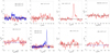 |
Fig. A.1 Main beam temperature, Tmb (K), versus velocity for [N II] spectra (red) at the OFF positions for eight LOSs from 20.°9 to 28.°7 at b = 0.°4. Superimposed on the [N II] spectra are the corresponding [C II] spectra (blue) from Herschel’s GOT C+ survey. [C II] was observed by GOT C+ at only two OFF positions above the plane, l = 20.°9 and 26.°1, at b = +0.°50. |
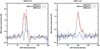 |
Fig. A.2 Main beam temperature, Tmb (K), versus velocity for [N II] for two of the four LOS where we had to correct the spectra for emission in the OFF position at b = 0.°4. The black line is the uncorrected spectrum at b = 0.°0, the blue line is the emission at b = 0.°4, and the red line is the corrected spectrum at b = 0.°0. |
In Fig. A.1, we plot [N II] for the OFF positions at b = 0.°4. There are only two [C II] OFF positions above the plane at b = 0.°5 that have [C II] spectra (the other GOT C+ HIFI OFF positions were observed below the plane). These [C II] OFF positions are not used here but are shown to indicate that [C II] is widespread above the plane, in most cases more so than [N II]. Four OFF positions (b = 0.°4) had no detectable [N II] at the level of the three times the rms noise (G020.9+0.4, G021.7+0.4, G024.3+0.4, and G025.2+0.4), one had strong emission (G023.5+0.4), and the remaining three had weak emission (G026.1+0.4, G027.0+0.4, and G028.7+0.4).
For the four LOS with [N II] emission in the OFF position we corrected the b = 0.°0 spectra by adding back the emission. In Fig. A.2, we show two examples, one for G023.5+0.0, which has the strongest emission at b = 0.°4, and one for a representative LOS, G026.1+0.0, which has weak emission at the OFF position, b =0.°4. The smallcorrection seen for the [N II] spectrum at G026.1+0.0 is typical of the other two LOS with weak emission, whereas at G023.5+0.0 the correction is significant.
Appendix B Thermal and turbulent linewidths derivation
The velocity dispersion of the RRL and [N II] lines can be written as,
 (B.1)
(B.1)
where, ΔVo, ΔVth, and ΔVturb are the observed, thermal, and turbulent Full Width Half Maximum (FWHM) line widths, respectively. For each species, we can write the thermal line width as,
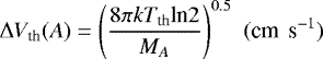 (B.2)
(B.2)
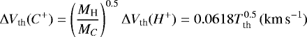
where A labels H+, C+, or N+, yielding,
 (B.3)
(B.3)
 (B.4)
(B.4)
 (B.5)
(B.5)
We assume that the [N II] (and where we use [C II]) emission arises from the same region as the RRL lines so that we can write Eq. (B.1) for both the H II and [N II] lines and, assuming that they have the same turbulent velocity dispersion and thermal temperature, ΔVturb(H+) = ΔVturb(N+). The solution for the thermal and turbulent velocity dispersions for RRL and [N II] lines, take the form,
![Mathematical equation: \begin{equation*}\Delta V_{\textrm{th}}(H^+)=\bigg (\frac{M_{\textrm{N}}}{M_{\textrm{N}}-M_{\textrm{H}}}\bigg)^{0.5}[\Delta V_{\textrm{o}}^2(H^+)-\Delta V_{\textrm{o}}^2(N^+)]^{0.5}\, (\textrm{km\,s}^{-1})\,\end{equation*}](/articles/aa/full_html/2021/07/aa40223-20/aa40223-20-eq29.png) (B.6)
(B.6)
 (B.7)
(B.7)
In the positions without detection of [N II] we can place a strict upper limit on the thermal temperatures from the width of the hydrogen RRL lines.
References
- Abel, N. P. 2006, MNRAS, 368, 1949 [NASA ADS] [CrossRef] [Google Scholar]
- Abel, N. P., Ferland, G. J., Shaw, G., & van Hoof, P. A. M. 2005, ApJS, 161, 65 [NASA ADS] [CrossRef] [Google Scholar]
- Accurso, G., Saintonge, A., Bisbas, T. G., & Viti, S. 2017a, MNRAS, 464, 3315 [NASA ADS] [CrossRef] [Google Scholar]
- Accurso, G., Saintonge, A., Catinella, B., et al. 2017b, MNRAS, 470, 4750 [NASA ADS] [Google Scholar]
- Anderson, L. D., Bania, T. M., Balser, D. S., & Rood, R. T. 2011, ApJS, 194, 32 [NASA ADS] [CrossRef] [Google Scholar]
- Anderson, L. D., Deharveng, L., Zavagno, A., et al. 2015, ApJ, 800, 101 [NASA ADS] [CrossRef] [Google Scholar]
- Anderson, L. D., Luisi, M., Liu, B., et al. 2021, ApJS, 254, 28 [CrossRef] [Google Scholar]
- Balser, D. S., Rood, R. T., Bania, T. M., & Anderson, L. D. 2011, ApJ, 738, 27 [NASA ADS] [CrossRef] [Google Scholar]
- Balser, D. S., Wenger, T. V., Anderson, L. D., & Bania, T. M. 2015, ApJ, 806, 199 [NASA ADS] [CrossRef] [Google Scholar]
- Bania, T. M., Anderson, L. D., Balser, D. S., & Rood, R. T. 2010, ApJ, 718, L106 [NASA ADS] [CrossRef] [Google Scholar]
- Bania, T., Wenger, T., Balser, D., & Anderson, L. 2016, TMBIDL: Single dish radio astronomy data reduction package [Google Scholar]
- Bennett, C. L., Fixsen, D. J., Hinshaw, G., et al. 1994, ApJ, 434, 587 [CrossRef] [Google Scholar]
- Brown, J. M., Varberg, T. D., Evenson, K. M., & Cooksy, A. L. 1994, ApJ, 428, L37 [NASA ADS] [CrossRef] [Google Scholar]
- Cooksy, A. L., Blake, G. A., & Saykally, R. J. 1986, ApJ, 305, L89 [NASA ADS] [CrossRef] [Google Scholar]
- Croxall, K. V., Smith, J. D., Pellegrini, E., et al. 2017, ApJ, 845, 96 [NASA ADS] [CrossRef] [Google Scholar]
- Durán, C. A., Güsten, R., Risacher, C., et al. 2021, IEEE Trans. Terahertz Sci. Technol., in press [arXiv:2012.05106] [Google Scholar]
- Esteban, C., & García-Rojas, J. 2018, MNRAS, 478, 2315 [NASA ADS] [CrossRef] [Google Scholar]
- Gerin, M., Ruaud, M., Goicoechea, J. R., et al. 2015, A&A, 573, A30 [NASA ADS] [CrossRef] [EDP Sciences] [Google Scholar]
- Geyer, M., & Walker, M. A. 2018, MNRAS, 481, 1609 [Google Scholar]
- Goldsmith, P. F., Y"i"ld"i"z, U. A., Langer, W. D., & Pineda, J. L. 2015, ApJ, 814, 133 [NASA ADS] [CrossRef] [Google Scholar]
- Graf, U. U., Simon, R., Stutzki, J., et al. 2012, A&A, 542, A16 [NASA ADS] [CrossRef] [EDP Sciences] [Google Scholar]
- Grenier, I. A., Casandjian, J.-M., & Terrier, R. 2005, Science, 307, 1292 [Google Scholar]
- Guan, X., Stutzki, J., Graf, U. U., et al. 2012, A&A, 542, L4 [NASA ADS] [CrossRef] [EDP Sciences] [Google Scholar]
- Guevara, C., Stutzki, J., Ossenkopf-Okada, V., et al. 2020, A&A, 636, A16 [CrossRef] [EDP Sciences] [Google Scholar]
- Haffner, L. M., Dettmar, R.-J., Beckman, J. E., et al. 2009, Rev. Mod. Phys., 81, 969 [NASA ADS] [CrossRef] [Google Scholar]
- Heyminck, S., Graf, U. U., Güsten, R., et al. 2012, A&A, 542, A1 [NASA ADS] [CrossRef] [EDP Sciences] [Google Scholar]
- Hoyle, F., & Ellis, G. R. A. 1963, Aust. J. Phys., 16, 1 [CrossRef] [Google Scholar]
- Johnson, J. A. 2019, Science, 363, 474 [NASA ADS] [CrossRef] [EDP Sciences] [Google Scholar]
- Kaufman, M. J., Wolfire, M. G., & Hollenbach, D. J. 2006, ApJ, 644, 283 [Google Scholar]
- Kingdon, J. B., & Ferland, G. J. 1996, ApJS, 106, 205 [NASA ADS] [CrossRef] [Google Scholar]
- Kirsanova, M. S., Ossenkopf-Okada, V., Anderson, L. D., et al. 2020, MNRAS, 497, 2651 [CrossRef] [Google Scholar]
- Kurtz, S. 2005, in IAU Symposium, 227, Massive Star Birth: A Crossroads of Astrophysics, eds. R. Cesaroni, M. Felli, E. Churchwell, & M. Walmsley, 111 [Google Scholar]
- Langer, W. D., & Pineda, J. L. 2015, A&A, 580, A5 [NASA ADS] [CrossRef] [EDP Sciences] [Google Scholar]
- Langer, W. D., Velusamy, T., Pineda, J. L., et al. 2010, A&A, 521, A17 [NASA ADS] [CrossRef] [EDP Sciences] [Google Scholar]
- Langer, W. D., Velusamy, T., Pineda, J. L., Willacy, K., & Goldsmith, P. F. 2014, A&A, 561, A122 [NASA ADS] [CrossRef] [EDP Sciences] [Google Scholar]
- Langer, W. D., Goldsmith, P. F., Pineda, J. L., et al. 2015, A&A, 576, A1 [NASA ADS] [CrossRef] [EDP Sciences] [Google Scholar]
- Langer, W. D., Goldsmith, P. F., & Pineda, J. L. 2016, A&A, 590, A43 [NASA ADS] [CrossRef] [EDP Sciences] [Google Scholar]
- Langer, W. D., Velusamy, T., Goldsmith, P. F., et al. 2017, A&A, 607, A59 [NASA ADS] [CrossRef] [EDP Sciences] [Google Scholar]
- Luisi, M., Anderson, L. D., Balser, D. S., Bania, T. M., & Wenger, T. V. 2016, ApJ, 824, 125 [NASA ADS] [CrossRef] [Google Scholar]
- Meijerink, R., & Spaans, M. 2005, A&A, 436, 397 [NASA ADS] [CrossRef] [EDP Sciences] [Google Scholar]
- Mizutani, M., Onaka, T., & Shibai, H. 2002, A&A, 382, 610 [NASA ADS] [CrossRef] [EDP Sciences] [Google Scholar]
- Nahar, S. N., & Pradhan, A. K. 1997, ApJS, 111, 339 [NASA ADS] [CrossRef] [Google Scholar]
- Oberst, T. E., Parshley, S. C., Nikola, T., et al. 2011, ApJ, 739, 100 [NASA ADS] [CrossRef] [Google Scholar]
- Persson, C. M., Gerin, M., Mookerjea, B., et al. 2014, A&A, 568, A37 [NASA ADS] [CrossRef] [EDP Sciences] [Google Scholar]
- Pineda, J. L., Langer, W. D., Velusamy, T., & Goldsmith, P. F. 2013, A&A, 554, A103 [NASA ADS] [CrossRef] [EDP Sciences] [Google Scholar]
- Pineda, J. L., Horiuchi, S., Anderson, L. D., et al. 2019, ApJ, 886, 1 [CrossRef] [Google Scholar]
- Planck Collaboration XIX. 2011, A&A, 536, A19 [NASA ADS] [CrossRef] [EDP Sciences] [Google Scholar]
- Reynolds, R. J. 1991, in The Interstellar Disk-Halo Connection in Galaxies, ed. H. Bloemen, 144, 67 [CrossRef] [Google Scholar]
- Risacher, C., Güsten, R., Stutzki, J., et al. 2016, A&A, 595, A34 [NASA ADS] [CrossRef] [EDP Sciences] [Google Scholar]
- Rolleston, W. R. J., Smartt, S. J., Dufton, P. L., & Ryans, R. S. I. 2000, A&A, 363, 537 [NASA ADS] [Google Scholar]
- Rubin, R. H. 1989, ApJS, 69, 897 [NASA ADS] [CrossRef] [Google Scholar]
- Samson, J. A. R., & Angel, G. C. 1990, Phys. Rev. A, 42, 1307 [NASA ADS] [CrossRef] [Google Scholar]
- Schöier, F. L., van der Tak, F. F. S., van Dishoeck, E. F., & Black, J. H. 2005, A&A, 432, 369 [NASA ADS] [CrossRef] [EDP Sciences] [Google Scholar]
- Sternberg, A., Hoffmann, T. L., & Pauldrach, A. W. A. 2003, ApJ, 599, 1333 [NASA ADS] [CrossRef] [Google Scholar]
- Tayal, S. S. 2008, A&A, 486, 629 [NASA ADS] [CrossRef] [EDP Sciences] [Google Scholar]
- Tayal, S. S. 2011, ApJS, 195, 12 [NASA ADS] [CrossRef] [Google Scholar]
- Velusamy, T., Langer, W. D., Pineda, J. L., & Goldsmith, P. F. 2012, A&A, 541, L10 [NASA ADS] [CrossRef] [EDP Sciences] [Google Scholar]
- Velusamy, T., Langer, W. D., Goldsmith, P. F., & Pineda, J. L. 2015, A&A, 578, A135 [NASA ADS] [CrossRef] [EDP Sciences] [Google Scholar]
- Voronov, G. S. 1997, Atomic Data Nuclear Data Tables, 65, 1 [NASA ADS] [CrossRef] [Google Scholar]
- Young, E. T., Becklin, E. E., Marcum, P. M., et al. 2012, ApJ, 749, L17 [NASA ADS] [CrossRef] [Google Scholar]
All Tables
All Figures
|
Fig. 1 Location of the eight LOSs observed in [N II], RRL, and [C II], indicated + signs, superimposed on a moment 0 integrated intensity map of the Hnα RRL GBT Diffuse Ionized Gas Survey (GDIG; Anderson et al. 2021). None of the LOS intersect the locations of the brightest compact emission, although many intersect larger ionized zones. |
| In the text | |
|
Fig. 2 Main beam temperature, Tmb (K) versus velocity for [N II] (red) and [C II] (blue) (right axis and scale) and the corresponding Hnα RRL spectra(black) Tmb (mK) (left axis and scale) for eight LOSs (G020.9+0.0 to G028.7+0.0) at b = 0.°0. [N II] was not detected at G025.2+0.0, and was marginally detected towards G021.7+0.0 at two velocities centered on ~25 and 67 km s−1. |
| In the text | |
|
Fig. 3 Intensity ratio of the 122–205 μm lines in W m−2 sr−1, versus electron density for kinetic temperatures Tkin (K) ranging from 2000 K to 20 000 K. The curves are labeled by Tkin (K) and employ the collisional de-excitation rate coefficients of Tayal (2011). |
| In the text | |
|
Fig. 4 Fractional abundance of N+, x(N+), derived from [N II] and the RRL emission lines. The values derived from GREAT are shown in black, while those from HIFI (in Table 3 Pineda et al. 2019) that are at the same Galactic latitude are plotted in red. |
| In the text | |
|
Fig. 5 Ratio of the population of the levels f3∕2(C+) to f1 (N+) as a function of electron density for kinetic temperatures in the range 2000–10 000 K. |
| In the text | |
|
Fig. 6 Main beam temperature, Tmb (K), versus velocity for [N II] spectra (red) and 12CO(1–0) (black) for the six LOS where [N II] was clearly detected. |
| In the text | |
|
Fig. 7 Fractional abundance of ionized nitrogen, f(N+), when the only operative processes are electron collisional ionization and recombination (blue) as a function of the plasma temperature, Tkin (K), compared to f(N+) when the only collisional processes are proton charge exchange and recombination (red). In a realistic case both processes occur simultaneously and the corresponding behavior for f(N+) is plotted asthe black curve. |
| In the text | |
|
Fig. 8 EUV photon flux required to maintain an ionized fraction of 50%, N+/N = 1, (blue curve) and 83%, N+/N = 5, (red curve) for a density of n(e) = 10 cm−3, when the only loss processes is electron recombination as a function of the plasma temperature, Tkin (K). The curves are proportional to density. |
| In the text | |
|
Fig. A.1 Main beam temperature, Tmb (K), versus velocity for [N II] spectra (red) at the OFF positions for eight LOSs from 20.°9 to 28.°7 at b = 0.°4. Superimposed on the [N II] spectra are the corresponding [C II] spectra (blue) from Herschel’s GOT C+ survey. [C II] was observed by GOT C+ at only two OFF positions above the plane, l = 20.°9 and 26.°1, at b = +0.°50. |
| In the text | |
|
Fig. A.2 Main beam temperature, Tmb (K), versus velocity for [N II] for two of the four LOS where we had to correct the spectra for emission in the OFF position at b = 0.°4. The black line is the uncorrected spectrum at b = 0.°0, the blue line is the emission at b = 0.°4, and the red line is the corrected spectrum at b = 0.°0. |
| In the text | |
Current usage metrics show cumulative count of Article Views (full-text article views including HTML views, PDF and ePub downloads, according to the available data) and Abstracts Views on Vision4Press platform.
Data correspond to usage on the plateform after 2015. The current usage metrics is available 48-96 hours after online publication and is updated daily on week days.
Initial download of the metrics may take a while.