| Issue |
A&A
Volume 651, July 2021
|
|
|---|---|---|
| Article Number | A29 | |
| Number of page(s) | 22 | |
| Section | Planets and planetary systems | |
| DOI | https://doi.org/10.1051/0004-6361/202039668 | |
| Published online | 06 July 2021 | |
Observations of distant comet C/2011 KP36 (Spacewatch): photometry, spectroscopy, and polarimetry
1
Astronomical Institute of the Slovak Academy of Sciences,
05960
Tatranská Lomnica,
Slovak Republic
e-mail: This email address is being protected from spambots. You need JavaScript enabled to view it.
2
Main Astronomical Observatory of the National Academy of Sciences,
27 Akademika Zabolotnoho St.,
03143
Kyiv,
Ukraine
3
Astronomical Observatory of Taras Shevchenko National University of Kyiv,
3 Observatorna St.,
04053
Kyiv,
Ukraine
4
University of Maryland,
College Park,
MD,
USA
5
Crimean Astrophysical Observatory,
Nauchnij,
Crimea
6
Special Astrophysical Observatory of the Russian Academy of Science,
Karachai-Cherkessia,
Nizhnij Arkhyz
369167,
Russia
Received:
13
October
2020
Accepted:
12
April
2021
Abstract
Aims. The main objective of our study is to obtain new observational results for the active long-period comet C/2011 KP36 (Spacewatch). This comet has unusual orbital properties and moves at distances larger than 5 au from the Sun.
Methods. We carried out extensive observations of comet C/2011 KP36 (Spacewatch) at the 6-m BTA telescope of the Special Astrophysical Observatory of the Russian Academy of Sciences with the focal reducer SCORPIO-2. We obtained quasi-simultaneous long-slit spectra in the visible, as well as photometric and linear polarimetric images with the g-sdss and r-sdss filters on November 25, 2016 when the heliocentric and geocentric distances of the comet were 5.06 au and 4.47 au, respectively. We modeled the behavior of the color and polarization in the coma, considering the dust as an ensemble of polydisperse nonspherical particles.
Results. Two strong jet-like structures in solar and antisolar directions and two short and narrow jet features in the perpendicular direction were revealed in the coma. Our simulations showed that the latter two jets originated from the same active area. We determined the orientation of the rotation axis of the nucleus and the position of three active areas. High activity of the comet was characterized by Afρ values of 1065 ± 11 cm in the g-sdss filter and 1264 ± 17 cm in the r-sdss filter. The comet was found to be rich in CO+, while there was no clear detection of CN, C3, C2, and N2+. The dust color g–r varies over the coma from about 0.2m to 0.7m, and the linear polarization degree from about −1% to −6% at the phase angle 9.6°. The color of the nucleus of comet C/2011 KP36 (Spacewatch) is ultrared, B – R = 1.9m ± 0.3m.
Conclusions. The high variability of the observed characteristics over the coma of comet C/2011 KP36 (Spacewatch) indicates significant and variable activity of the nucleus with, probably, numerous small active areas. Together with the three identified large active areas, they are characterized by different combinations of water ice, CO2 ice, and refractory dust and sizes of their particles, which are in the micron-size range.
Key words: comets: general / comets: individual: C/2011 KP36 (Spacewatch) / polarization / scattering / methods: miscellaneous
© ESO 2021
1 Introduction
The object C/2011 KP36 (Spacewatch) was discovered within the Spacewatch project by T. H. Bressi on May 21, 2011 at the Steward Observatory (Kitt Peak) using the Spacewatch 0.9 m telescope. It was originally classified as asteroid 2011 KP36 (Bressi et al. 2011). The detected object of 20.4 magnitude moved at distances of 12.43 au and 11.48 au from the Sun and the Earth, respectively. However, on April 19, 2012 (at about 10.8 au), it started to display a cometary appearance; it was diffuse, with a coma 6′′ in diameter and a faint tail 9′′ in the direction of position angle PA ≈ 10° (Bressi et al. 2012). As a result, the object was named comet C/2011 KP36 (Spacewatch) (hereafter 2011KP36) (Buzzi et al. 2012). The current orbital parameters of the comet are summarized in Table 1, which displays the unique orbital properties of the object. The orbital calculations showed that 2011KP36 is a long-period comet with a perihelion distance of q = 4.88 au (the perihelion passage was on May 26, 2016) and an aphelion distance of Q = 71.94 au, which is twice the aphelion distance of Neptune (aN = 30.33 au). Thus, its highly eccentric, moderately inclined orbit extends beyond the orbit of Neptune. Given the unique orbital properties of 2011KP36, it is very important to correctly classify this object.
According to the NASA/Horizons service, comet 2011KP36 belongs to the Jupiter family of comets (JFCs). However, JFCs are defined as having a Tisserand parameter with respect to Jupiter 2 < TJ < 3 and a traditional constraint of orbital period P < 20 yr (a < 7.4 au) (Dones et al. 2004). Since comet 2011KP36 has a Tisserand parameter of TJ = 2.64 and P = 238 yr, it cannot belong to the JFCs. Bauer et al. (2013) attributed this comet to the group of scattered disk objects (SDOs), but it cannot be a scattered disk object as its perihelion is < 30 au. Given its eccentricity (e = 0.873), orbital period, and semi-major axis together with its Tisserand parameter, object 2011KP36 can be classified either as a Halley-type comet with orbital periods between 20 and 200 yr or a long-period comet with 7.4 < a < 40 au (Dones et al. 2004). For both types, the Tisserand parameter is TJ < 2. However, we lean to the conclusion made by Y. R. Fernández1 that comet 2011KR36 belongs to the “group of long-period comets that are nearly Halley-type” (LPC-HT) that have 200 < P < 250 yr and TJ < 2, despite the fact that for this comet TJ = 2.64.
There are not many publications regarding comet 2011KP36, because of the lack of extensive observational data. According to Bauer et al. (2013), the diameter of the cometary nucleus is 55.1 ± 19.4 km, the geometric albedo pV = 0.101 ± 0.062, and the absolute magnitude HV = 9.4m. A significant level of activity of the comet at large heliocentric distances resulted in rather high dust production, Afρ = 1435 cm at r = 8.478 au and 1141 cm at 8.212 au (Sárneczky et al. 2016). The slope parameter describing the profile of the coma brightness was negative for the first observation (−0.19) and positive for the second date (0.03), which suggests variations in matter production. However, observation of comet 2011KP36 before perihelion on July 18, 2015, at distances r = 5.38 au and Δ = 4.49 au, showed a fairly high level of activity: Afρ = 4444 cm within the aperture of ρ ≈ 104 km centered on the optocenter of the comet (Garcia et al. 2020).
In this paper, we present the results and analysis of optical observations of comet 2011KP36 obtained at a post-perihelion distance of 5.06 au. The paper is organized as follows: specific details of our observations and data reduction are described in Sect. 2; the results obtained from spectroscopy, photometry, and polarimetry and their comprehensive analysis are given in Sects. 3–9; the results of numerical modeling of the spatial variations of polarization and color are presented in Sect. 10; discussion of the results and a summary are given in Sect. 11.
Current orbital parameters of comet C/2011 KP36 (Spacewatch).
2 Observations and data reduction
We observed comet 2011KP36 on November 25, 2016, after the perihelion passage when the heliocentric and geocentric distances of the comet were 5.06 au and 4.47 au, respectively. For observations, the multimode focal reducer SCORPIO-2 attached to the prime focus of the 6-m Big Telescope Alt-azimuth (BTA) of the Special Astrophysical Observatory of the Russian Academy of Sciences (SAO RAS) was used. The instrument is described in detail by Afanasiev & Moiseev (2011) and Afanasiev & Amirkhanyan (2012). The observations of the comet were conducted in the packet mode, which allowed us to make a sequence of exposures to obtain direct CCD images (hereafter called Image), spectra with a long slit (Sp), and imaging linear polarimetry (ImageLP). We used the CCD chip E2V-42-90 with 2K × 4K square pixels of 16 μm corresponding to 0.18′′ (584 km px−1) on the sky plane without binning. The full field of view of the CCD is 6.1′ × 6.1′. The telescope was tracked on the comet to compensate for its apparent motion during the exposure. The transparency of the sky during the night was very good, but sometimes there were passing clouds. Therefore, the seeing ranged from 1.2′′ (for most exposures) to 2.6′′, that is from 3 890 to 8 429 km at the comet, as determined from the full width at half maximum (FWHM) of the observed standard stars.
Photometry and polarimetry of comet 2011KP36 were performed through the Sloan Digital Sky Survey (SDSS) g-sdss (the central wavelength λ0 and FWHM are λ4650/1300 Å) and r-sdss (λ6200/1200 Å) broadband filters (see Table 2). Observations of the twilight sky through the same filters were also performed to provide flat-field corrections. To increase the signal-to-noise ratio (S/N) of the measured signal, we applied a 2 × 2 binning to the original polarimetric and photometric images prior to reduction and analysis. Therefore, the scale was 0.36′′/px. The background sky was estimated using an area in the image free from contamination from the coma and background stars. The S/N varied on average from about 50 in the near-nucleus coma to about 7 in the outer region of the coma, at a distance of 85 000 km.
We derived spectra of the comet with a long-slit mask. We used the transparent grism VPHG940@600 as a disperser in the spectroscopic mode of the SCORPIO-2. The slit of 6.1 arcmin × 1.0 arcsec was placed on the nucleus position in the sky and oriented along the velocity vector of the comet. The obtained spectra covered the wavelength range 3500–7000 Å and had a dispersion of 1.16 Å px−1. The spectral resolution of spectra, defined by slit width, was 7 Å. We applied 1 × 2 binning to all spectroscopic images. The wavelength calibration was made using the spectrum of a He–Ne–Ar lamp. We used a smoothed spectrum of an incandescent lamp to provide flat-field corrections for the spectral data.
To provide an absolute flux calibration of the photometric and spectral measurements, we observed spectrophotometric standard stars Feige 56 (Oke 1990). The spectral atmospheric transparency values for the SAO RAS were taken from Kartasheva & Chunakova (1978). We made standard reduction manipulations regarding the obtained spectroscopic data. We used the regions of the slit that were free of the cometary coma to estimate the level of the sky background, which was then subtracted from the image.
For measurements of the degree of linear polarization of the comet, we used the dichroic polarization analyzer (called POLAROID), which was positioned in three fixed positions at angles +60°, 0°, and − 60° (Afanasiev & Amirkhanyan 2012). Using the intensities measured at these angles, we calculated the Stokes parameters q and u, normalized to the total intensity, at each point of the image. To determine the instrumental polarization and the correction for the zero-point of the position angle of the polarization plane, we observed the polarized and nonpolarized standard stars with well-known large interstellar polarization taken from the lists of Hsu & Breger (1982), Schmidt et al. (1992), and Heiles (2000). Typically, the instrumental polarization was less than 0.1%. The errors in the measured polarization degree of the comet varied between 0.12% and 1.1%.
The specialized software packages in the IDL (Interactive Data Language) environment developed in the SAO RAS were used to perform the primary reductions of the observational data. This included bias frame subtraction, division of the science frames by flat fields, removing the traces of cosmic rays from calibration images (bias, dark, and flat images), and preparation of images for processing. The parts of the image free of the cometary coma and faint stars were used to estimate the level of sky background using the procedure of building a histogram of counts in the image. The maximum count was chosen as the background sky level, which was then subtracted from the image. To increase the S/N, the individual images were stacked together and summed using a robust averaging method (Rousseeuw & Bassett 1990). We used this method because it is more stable in respect to random errors and allows us to calculate an unbiased average of the measured values (Maronna et al. 2017).
In the case of long-slit spectroscopy, the data reduction included the bias frame subtraction, removal of cosmic ray tracks, flat-field correction with the spectrum of a built-in lamp with a continuous spectrum, geometrical correction along the slit, correction of the spectral line curvature, sky background subtraction, spectral wavelength calibration, and the presentation of data with uniform scale spacing along the wavelengths. The night-sky spectrum was removed using its level measured in each column over the zones free of the cometary coma.
A detailed description of processing the photometric, spectral, and polarimetric data and the method for calculating polarization parameters with SCORPIO-2 can be found in Afanasiev & Amirkhanyan (2012), Afanasiev et al. (2014), Ivanova et al. (2009, 2017, 2019), and Rosenbush et al. (2017).
Information about the observations of comet 2011KP36 is presented in Table 2, where we list the observation date (the mid-cycle time, UT), the heliocentric (r) and geocentric (Δ) distances, the phase angle of the comet (α), the position angle of the scattering plane (φ), the filter or grating, the total exposure time (Texp), the number of observation cycles (N), and the mode of the observations.
Log of the observations of comet C/2011KP36 (Spacewatch).
3 Spectrum of the comet
One of the goals of our program of distant comet observations is to study the energy distribution in the cometary spectra and search for possible molecular emissions. To increase the S/N, we coadded the available spectra and collapsed the counts in the spatial direction within ± 25′′ from the optocenter. Figure 1 shows a stepwise transformation of the observed spectrum of comet 2011KP36 (a) to the continuum (a, b) and emission spectrum (c). The derived energy distribution in the observed cometary spectrum along dispersion is shown in Fig. 1 a (black line). Since the Solar spectrum (Neckel & Labs 1984) has very high resolution, it was convolved with an appropriate instrumental profile to the cometary spectrum resolution and normalized to the flux of the comet around 5000 Å. The obtained spectrum is superimposed on the observed spectrum of the comet (red line). To isolate the emission spectrum of the comet (Fig. 1 c), we subtracted the fitted continuum (Fig. 1 b) from the observed spectrum.
Figure 2 presents the 3880–5200 Å wavelength range of the observed spectrum of comet 2011KP36 in an enlarged scale, where the strongest emissions of CN, C3, C2, and CO+ are expected. There is also the calculated spectrum of CO+. The emissions (2, 0), (1, 0), (2, 1), and (1, 1) of the vibrational transitions of CO+ (A2Π–X2Σ) band system are clearly seen in Fig. 2. However, the spectrum does not show any emission features from the CN, C3, C2 carbon-bearing molecular species. Therefore, using the transmission curves for the Hale-Bopp (HB) narrowband filters (Farnham et al. 2000), we only determined upper limits to the fluxes of these emissions and their production rates. For this, we used the same technique that was applied to the spectrum of comet C/2014 A4 (SONEAR) (Ivanova et al. 2019). These values have been computed with an aperture of 1.56′′ (5057 km). In Table 3, we provide the results of our calculations, where λ/Δλ is the central wavelength with the bandpass of the appropriate narrowband comet HB filters (Farnham et al. 2000), F is the full flux inside a specified aperture, and Q is the gas production rate.
The CN emissions were observed in comets even at larger heliocentric distances. For example, CN was observed in Chiron at a record heliocentric distance of 11.3 au (Bus et al. 1991), at 9.8 au in comet C/1995 O1 (Hale-Bopp) (Rauer et al. 2003), at 6.8 au in comet C/2002 VQ94 (LINEAR) (Korsun et al. 2006, 2008), and in comet 29P/Schwassmann-Wachmann 1 at r > 5.5 au from the Sun (Korsun et al. 2008; Ivanova et al. 2016, 2018). There are only two cases when C3 emission was observed at large heliocentric distances, namely, at 7.0 au in comet C/1995 O1 (Hale-Bopp) (Rauer et al. 2003) and in comet C/2002 VQ94 at 6.8 au (Korsun et al. 2006). The emission bands from C2 molecules (Swan bands) were only once detected at a relatively large heliocentric distance, 4.7 au, in comet C/1995 O1 (Hale–Bopp) (Rauer et al. 1997).
So far, CO+ has only been detected in comet 29P/Schwassmann-Wachmann 1, at r ≤ 6.2 au (Larson 1980; Cochran et al. 1982; Korsun et al. 2008; Ivanova et al. 2016, 2018) and in comet C/2002 VQ94 (LINEAR) at heliocentric distances from 6.8 to 8.36 au (Korsun et al. 2006, 2008, 2014).
The spectrum of comet 2011KP36 (Fig. 1) shows that the dust reflectivity, S(λ), is almost constant to approximately 5300 Å, and then gradually increases (Fig. 1b). We determine S(λ) as the ratio of the comet spectrum Fc(λ) to the scaled Solar spectrum Fsun(λ): S(λ) = Fc(λ)∕Fsun(λ). We follow A’Hearn et al. (1984), employing the normalized gradient of reflectivity:
 (1)
(1)
where S(λ1) and S(λ2) correspond to the dust reflectivity at wavelengths λ1 and λ2 under the condition λ2 > λ1. We express S′(λ1, λ2) in percent per 1000 Å. We used central wavelengths of g-sdss and r-sdss filters for λ1 and λ2. As a result, we obtained the spectral gradient of reflectivity, which is equal to 11.9 ± 2% per 1000 Å in the wavelength range 4650–6200 Å. Most distant comets are redder than the Sun, with average values from 10 to 22% per 1000 Å (Storrs et al. 1992; Kulyk et al. 2018; Ivanova et al. 2019).
Upper limits to the emission fluxes and production rates for undetected species CN, C2, and C3 in the spectrum of comet C/2011 KP36 (Spacewatch).
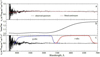 |
Fig. 1 Long-slit spectrum of comet C/2011 KP36 (Specewatch) derived on November 25, 2016. (a) Energy distribution in the observed spectrum of the comet (black line) and the scaled Solar spectrum taken from Neckel & Labs (1984) (red line); (b) polynomial fitting of the cometary spectrum/Solar spectrum ratio; and (c) emission spectrum of the comet derived by subtracting the fitted continuum from the observed spectrum and the transmission curves of the g-sdss and r-sdss filters. |
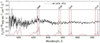 |
Fig. 2 Emissions of CO+ identified in the observed spectrum of comet C/2011 KP36 (Spacewatch). Calculated spectra of CO+ emissions are displayed at the bottom of the plot. |
4 Dust coma morphology
4.1 Observed morphology of the comet
We constructed intensity maps (Fig. 3 a) by stacking all the photometric images obtained with the same g-sdss filter (top panel) and separately with the r-sdss filter (bottom panel). The relative intensities of adjacent contours of isophots differ by a factor of  . The cometary coma is strongly asymmetric and elongated along the velocity vector of the comet that is close to the solar and antisolar directions. Its shape is very similar to the coma that Korsun et al. (2016) observed in comet P/2011 P1 (McNaught) at a heliocentric distance of 5.43 au.
In order to reveal the low-contrast structures in the dust coma of comet 2011KP36, the images were treated with digital filters (see Figs. 3b–e). We applied a combination of four numerical techniques and visual inspection: a rotational gradient method (Larson & Sekanina 1984), 1/ρ profile, azimuthal average, and renormalization methods (Samarasinha & Larson 2014). The two first techniques enabled us to remove the bright background from the cometary coma and highlight the low-contrast features. Division by azimuthal average is very effective to separate brighter broad jets. The different enhancement techniques affect the image in different ways, and to exclude spurious features the enhanced images were compared to each other. This means that we applied each technique to all individual frames separately, as well as to the same composite image, to evaluate whether revealed features are real or not. We also studied the change in the jet structure due to the shift in the comet’s optocenter. Previously, this technique was used to pick out structures in several comets with good results (Ivanova et al. 2009, 2016, 2017, 2018, 2019; Rosenbush et al. 2017; Picazzio et al. 2019).
In processed images, we revealed two strong jet-like structures close to the solar and antisolar directions of the coma, labeled as J1 and J2 in Fig. 3b, and two faint, short, and narrow jet features in the direction almost perpendicular to the Sun-comet direction, marked as J3 and J4 in this figure. The position angles (PA), measured counterclockwise from the north through the east, of the J1, J2, J3, and J4 are 261°, 103°, 188°, and 8°, respectively, while for the direction to the Sun PA = 241.5°. The J1 and J2 jets were bounded by the boundary of the cone swept out due to the rotation of the nucleus. Most probably, the observed coma in comet 2011KP36 was formed due to the activity of several isolated areas located on the cometary nucleus. Observation of this comet before perihelion passage on July 18, 2015 showed a similar morphology of the coma resembling corkscrews (Garcia et al. 2020).
4.2 Modeling the dust structures
The presence of jet-like structures in the coma can be an indication of localized active areas on the nucleus surface of comet 2011KP36. In order to reproduce the observed jet morphology, we used a simple geometrical model, the theoretical description of which is given in Appendix A. Recently this model was used for modeling the dust jets and fan in comet 2P/Encke (Rosenbush et al. 2020). The proposed model accounts for the orientation of the nucleus spin axis and its rotation period, the location of the active source on the nucleus, and the relative position of the Sun, Earth, and the comet. We assume that the nucleus is spherical and that the outflow of matter occurs radially from the active area and with a constant velocity only under the Sun’s illumination. Dispersion of the velocities of particles ejected from the nucleus and their acceleration under Solar radiation are not taken into account. A sequence of calculated model jets projected onto the plane of the sky shows the motion of the ejected matter and jet evolution in time. Such an approach is valid at small distances from the cometary nucleus. In the case of comet 2011KP36, this distance did not exceed 8000 km.
Since Solar radiation pressure (SRP) affects particles at any distance, it is important to know how much particle trajectories deviate at distances up to 8000 km due to the acceleration of the particles by SRP compared to the uniform motion that is considered in the proposed model. Vincent et al. (2010) estimated the effect of SRP on dust particles of about 1 micron in size that formed steady structures. According to their calculations, the ratio of SRP to Solar gravity, β, is equal to 0.4. For aheliocentric distance of about 5 au, at which we observed comet 2011KP36, the acceleration of particles by SRP for β = 0.4 should be 9.6 × 10⁻⁵ m s−2. If the particle ejection velocity is 0.1 km s−1, then a typical time to cover the distance of 8000 km is 8 × 10⁴ s. During this time, the deviation due to the acceleration of particles by SRP should be about 320 km, which does not affect the position of the particle in our image because this deviation corresponds to approximately 1/3 of a pixel, and, thus, has no noticeable effect on the shape of the jets.
The model calculations showed that the presence of three active areas on the nucleus of comet 2011KP36 was necessary to reproduce the observed jet structure. Under the assumption of continuous ejection of the dust particles, we studied the conditions, which can lead to the observed jet-like structures. The results of our modeling are shown in Fig. 4. We have found that the projected spin axis of the nucleus lies nearly in the sky plane (an inclination is approximately 15°) and is located along the direction J1–J2. In this case, active areas Source 1 and Source 2 form J1 and J2 jets, respectively. Jets J3 and J4 are formed by a single active area, Source 3, located near the equator of the cometary nucleus. The visible separation into two features, J3 and J4, is a result of the nucleus rotation and the projection of the particle flow ejected from the nucleus. The active area Source 3 has a lower activity compared to the other two areas, Source 1 and Source 2, located in the polar zones of the cometary nucleus.
The coordinates of the north pole of the rotation axis could not be accurately determined from a single image, but the model allowed us to obtain two solutions that gave a similar picture of the jets (see Fig. 4). There is a distinction in the direction of the rotation axis and, accordingly, in the latitudes of the active areas on the nucleus that form the observed jets J1 and J2. The coordinates of the rotation axis of the nucleus and the location of the active areas on the cometary nucleus are presented in Table 4.
We also simulated the case when the axis of rotation lies in the sky plane and is directed along jets J3–J4, that is, the axis of rotation is perpendicular to the one that provided the first solution. In this case, the more powerful jets J1 and J2 are no longer located in the equatorial region, and jet J1 coincides with the direction to the Sun. However, the simulation shows that in this case the observed configuration of the jets is poorly reproduced, and some important features of the jet profiles (see Sect. 9.2) cannot be reproduced. Besides, if the rotation axis is located in the picture plane and jets J3 and J4 are formed in different areas of the nucleus, then it is difficult to explain the relationship between the color variations in jets J3 and J4 (see Sect. 9.2).
Analysis of the surface brightness distribution in the coma shows that the second solution 2 from Table 4 is more likely. According to the measurements (Fig. 3b), jet J3 has a higher intensity compared to jet J4, although our modeling shows that they are formed by a single active area, Source 3 on the nucleus. This may be explained by the fact that the ejection of matter in the J4 direction occurred earlier, when the active area came out of the shadow during the rotation of the nucleus. In this case, the active area is less heated and, thus, less active. Similarly, if we analyze the geometry of jets J1 and J2, we see that they deviate from the rotation axis of the nucleus. The outflow rate of matter increases as the active areas Source 1 and Source 2 are heated, which corresponds to the visible displacement of jets J1 and J2 in the image towards the direction of nucleus rotation. Such conditions of the projection of jets on the picture plane do not allow us to estimate the emission velocity of matter. However, it is possible to determine a characteristic scale, which is the product of the rotation period and the velocity of material outflow. For the date of observations, it was (1.33 ± 0.12) × 104 km.
Figure 5 schematically represents various locations of active areas on the cometary nucleus during its rotation (Pn is the full period of nucleus rotation) as seen by an observer and the corresponding images of model jets on the plane of sky. The illuminated nucleus hemisphere is in the observer’s field of view. The model assumes that when the active area is on the illuminated side of the nucleus, an intense outflow of matter from this region occurs, forming the jets as shown in Fig. 5. Since we assume that there is no outflow of matter from the active areas on the night (dark) side of the nucleus, modeled jets are not formed at that time and we see gaps in the model jets, while the visible part of the jet moves away from the nucleus.
In Fig. 4a, one can see a wave structure in the J4 jet. The origin of this structure can be explained by precession of the spin axis; as a result, the position of the rotation axis of the nucleus periodically changes in space. The cause of precession is the presence of an external torque that acts on the nucleus. Such an external torque may be the jet force arising due to asymmetrical ejection of matter from the surface of the nucleus (Whipple & Sekanina 1979). The wave structure formed by the equatorial active area Source 3 can be described by the expression
 (2)
(2)
where Y and X are the distances along the rotation axis and perpendicular to it, ε is the angular radius of precession, Lp is the characteristic length of the precession that is equal to the product of the dust velocity and the precession period, and φ is the initialangle for a given moment of observation. Using the optimization method based on the least squares criterion applied to points of the observed wave structure and Eq. (2), we calculated the parameters of Eq. (2) for the wave structure in jet J4, namely the amplitude of precession ε = 6.0° ± 0.6° and the characteristic length Lp = (3.0 ± 0.15) × 104 km. The modeled wave structure is shown in Fig. 4b.
The wave structure of the J4 jet, produced by the active area Source 3, is better visible at its remote part on the g-sdss image (Fig. 4). The reasons for this may be the overlapping of the substance ejected from the rotating nucleus at different times and an increase of the wave amplitude with distance from the nucleus (according to Eq. (2)). At the same time, the J3 jet, produced by the same active area as J4, does not show the presence of a wave structure. We suggest that the J4 jet was formed by a cold active area, when Source 3 entered the hemisphere illuminated by the Sun. Although the J3 jet was formed by the same area, but it was already heated for half the period of the nucleus rotation. The change in the temperatureof the active area leads to changes in the characteristics of the dust particles in jets, which makes J3 brighter than J4 and affects the color of jets J3 and J4 (see Sect. 9.2). It is quite admissible that the dispersion of the sizes (and the velocities) of the dust particles increases for the jet arising from the heated area. This leads to a smearing of the wave structure in the entire J3 jet. The wave structure is not observed in the g-ssds image of the J4 jet (3b) due to much lower surface brightness in this filter and, hence, a low S/N.
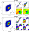 |
Fig. 3 Intensity maps of comet C/2011 KP36 (Spacewatch) in the g-sdss and r-sdss filters. (a) Direct images of the comet with the isophots differing by a factor |


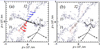 |
Fig. 4 Images of comet C/2011 KP36 (Spacewatch) in the r-sdss filter processed by a rotational gradient method. (a) Comparison of the observed (gray contours) and model jets: J1 is shown by red circles, J2 by blue circles, J3 and J4 by black circles. (b) Comparison of the observed and the modeled wave structure in the J4 jet (black). Directions to the Sun (⊙), north (N), east (E), and the negative velocity vector of the comet (V) are also provided. Negative distance is in the solar direction, and positive distance is in the antisolar direction. |
Best solutions for the coordinates of the north rotation pole of the nucleus of comet C/2011 KP36 (Spacewatch) and the cometocentric latitudes of the active areas.
5 Surface brightness profiles of dust
To describe the dust brightness as a function of cometocentric distance, we derived the radial profiles of the surface brightness for each jet-like structure observed in the g-sdss and r-sdss images of the multicomponent coma of comet 2011KP36 (Fig. 6). The cuts were made from the photometric center of the comet along the structures J1, J2, J3, and J4 and through the coma in the directions with the position angles 56°and 236°, namely, between jets J3 and J2 in the antisolar direction and between J1 and J3 in the solar direction. The individual curves show variations of the average flux in the 3 × 3 px size aperture with increasing cometocentric distance ρ. The brightness profiles are affected by seeing effects; therefore, the near-nucleus region (up to ~ 2240 km) was excluded from the analysis. Both plots show a slow flattening of the surface brightness profile beyond ~ 20 000 km. We manually selected the linear segment at the profile, and it was linearly approximated in the log–log plane. The distance ranges were fixed for all jets and the coma, and the method of determination of the slope of the radial profiles was the same for each structure. In Table 5, we present the best-fitting slopes to the linear fit of the radial brightness profiles in the g-sdss and r-sdss images of comet 2011KP36 for the range approximately 3.7< logρ < 4.2, which is between 5500 km and 16 500 km projected radial distance from the nucleus. Except for a limited central region, the profiles along the jets are flatter than the canonical profile 1/ρ expected in the case of a steady and isotropic emission of long-lived grains. Dust brightness profiles versus ρ in log–log representation are relatively well fitted, within error bars, with the slopes being between 0.55 and 0.79. The profiles in the solar direction (jets J1, J3, and the coma C1, PA = 236°) are steeper than those (jets J2, J4, and the coma C2, PA = 56°) in the antisolar direction (J2). Furthermore, steeper profiles are observed in the r-sdss filter.
Examining Fig. 6 and Table 5, we can see that the brightness varies not according to ρ−1 expected in the case of isotropic emission of dust from the nucleus. Actually, for a steady-state and free expansion of long-lived grains, the n value in the dependence I ∝ 1∕ρn should be –1. In this equation, I is the brightness of the coma and n is the dimensionless slope in log I versus logρ dependence,which describes the brightness variations with cometocentric distance ρ. For most comets, especially for the outer regions of the coma, the radial profiles of surface brightness are steeper than described by n = –1. However, in some cases (e.g., O’Dell et al. 1988), radial profiles of surface brightness can be flatter, that is, ∣ n∣ < 1. According to Jewitt (1991), such flat profiles may be a consequence of the time-variable emission from the nucleus. Therefore, we can assume that there is no steady state and free expansion of the dust from the nucleus of comet 2011KP36 that forms the coma and jets.
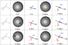 |
Fig. 5 Schematic representation of the nucleus of comet C/2011 KP36 (Spacewatch) together with the rotational axis as viewed from the Earth and the model jets obtained during various phases of the nucleus rotation assumed for the moment of observations on November 25, 2016. The red spot is the active area located at the north hemisphere of the nucleus at the cometocentric latitude +75° (Source 1), and the active area at the south hemisphere at latitude −78° (Source 2) is depicted as a blue spot. The active area at the south hemisphere at latitude −5° (Source 3) is depicted as a black spot. The bright area is the area illuminated by the Sun at the moment of observation. A full period of the nucleus rotation is denoted by Pn and T denotes the rotational phase as a part of the rotation period. The arrows indicate the direction to the Sun (⊙), north (N), east (E), and anti-velocity vector of the comet in projection on the sky (–V). |
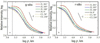 |
Fig. 6 Observed surface brightness profiles of comet C/2011 KP36 (Spacewatch) in log–log representation for flux calibrated images acquired in g-sdss (a) and r-sdss (b) bands. The individual solid curves are cross-cuts measured from the photometric center of the comet through the coma along jets J1, J2, J3, and J4, while the cuts through the coma centered in the antisolar (PA = 56°) and solar (PA = 236°) directions are marked as the dashed lines. The innermost data points that may be affected by seeing, bounded by a vertical dotted line, were not considered. Short black lines represent the canonical profile, in which the brightness varies with cometocentric distance ρ as I ∝ 1∕ρ. |
Power index n in the dependence I ∝ 1∕ρn measured in the g-sdss and r-sdss images of comet C/2011 KP36 (Spacewatch).
6 Contribution of the nucleus to the total brightness
Previous studies of comets, for example those of comet Encke (Rosenbush et al. 2020), showed that light scattered by the nucleus, especially if it is as large as that of comet 2011KP36, can strongly affect the observed characteristics of the coma at the first few thousand kilometers from the nucleus. Therefore, we decided to determine the possible contribution of the nucleus brightness to the total brightness of the coma of comet 2011KP36. For this, we used the method of fitting the model surface brightness to the observed images developed by Lamy et al. (2011), which was already successfully applied by us to comet 2P/Encke in Rosenbush et al. (2020).
The observed brightness distribution in the near-nucleus region is a sum of the fluxes from the coma and nucleus. We defined the contribution of each of these two components using a seeing-convolved image of a model comet that possessed the same image scale and point spread function (PSF) as the observed profiles. The visible brightness distribution from a point source was determined as the average from several images of field stars. We have compared the brightness profile of the comet with the averaged profile of field stars (Fig. 7), which is a proxy for the PSF of the telescope. In this case, the model brightness distribution of the comet can be represented by a two-dimensional convolution,
 (3)
(3)
where ⊗ is the convolution operator. We have adopted a relatively simple model of the coma, in which its surface brightness Icoma varies according to the power law
 (4)
(4)
where n is the power exponent in the model coma, and kc is the scaling factor for the coma in the model. The angular size of the nucleus at the distance of the comet is much smaller than the resolution of the telescope. Therefore, we represent the nucleus brightness Inucl using the Dirac delta function δ(ρ) and in the adopted model it can be written as
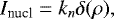 (5)
(5)
where Inucl is the brightness of the cometary nucleus, equal to the PSF scaled by the factor kn. To take into account the real resolution (seeing) during the observations, we use the averaged star profile, which corresponds to the PSF of the telescope. Thus, we have created images of model comets that possess the same image scale and PSF as the observed data, so that model profiles and real profiles can be directly compared.
In Fig. 7, we compare the radial cross-cuts through the intensity images derived in the g-sdss and r-sdss filtersfrom the optocenter of the comet along jets J1 and J2, J3, and J4, and a field star. The fluxes of the comet and star have been normalized to unity to compare how the profiles change with the distance from the nucleus and to search for any distinctions between the profiles. It turned out that the surface brightness profiles of comet 2011KP36 measured in the g-sdss and r-sdss images significantly differ. In the r-sdss filter, the profiles are only slightly more extended than the instrumental PSF at distances to approximately 10 000 km, with little of the extension in the solar direction, while there is a larger excess of brightness in the “wings” of the comet profiles. At the same time, the spatial brightness profiles of the comet in the g-sdss filter significantly exceed the star profile in all directions, but an especially large excess of brightness is observed in the solar direction, including the near-nucleus region. This implies that the contribution of the nucleus to the total coma brightness for the central pixels of the image in the g-sdss filter is much smaller than in the r-sdss filter.
To account for the significant asymmetry of the coma of comet 2011KP36, the model was upgraded. Two power exponent parameters were introduced: n− and n+ for the solar and antisolar directions, respectively. The parameters kc, kn, n−, and n+ were determined by the least squares method, minimizing the residuals between the model and observed profiles of stars. For analysis, we selected two brightness profiles located along jet J1 (position angle PA = 8°) and jet 4 (PA = 226°) and two profiles of the coma outside the jets (PA = 56° and 146°). All these profiles pass through the optocenter, forming solar–antisolar directions. The results of the model computations for the g-sdss and r-sdss images are given in Table 6. This table presents the position angle of profile PA; the power exponents n− and n+; the coefficient of proportionality for the nucleus kn in the model, determined by the least squares method minimizing the residuals between the modeled and observed profiles; the fraction of the comet’s flux from the nucleus to the central pixel intensity f0; the fraction of the central pixel in the total brightness of the nucleus fn; the fraction of the comet’s flux from the nucleus to the integral intensity of the coma with radius 5000 km fn (5000); and the error (obs-model) that is the root-mean-square (RMS) error of the difference between the observed and modeled brightness distribution.
The results of our modeling are also shown in Fig. 8. Here we show the observed and modeled brightness profiles centered at the central pixel along four different directions, including jets J1 and J4 and cross-cuts through the ambient coma. Model calculations of spatial profiles along four directions in the coma give close values of the nucleus contribution to the total intensity of the central pixel, with an average value of 0.17 ± 0.03 for the g-sdss image. For the r-sdss image, the contribution of the nucleus is significantly higher, on average 0.42 ± 0.05, hence, there is a strong dependence on the transmission band of the filter. Table 6 also shows that the nucleus contribution to the comet flux within a circular aperture of a radius of 5000 km is considerably higher in the r-sdss filter. Therefore, for the central pixel in the g-sdss filter, the nucleus magnitude is about 1.9m fainter thanthe total magnitude, whereas in the r-sdss filter this value is only about 0.9m. If we take the 5000 km near-nucleus area of the coma, the nucleus magnitude is 2.0m (g-sdss) and 1.0m (r-sdss) fainter than the integral magnitude of the selected area. Apparently, this large difference can be explained by the extremely red color of the nucleus of comet 2011KP36 that we found in Sect. 7.1.
As Table 6 shows, the power exponents for spatial coma profiles in different directions are smaller than 1 for both filters, that is ∣ n∣ < 1, which are close to the powerindex n obtained in Sect. 5 for distances between 5500 km and 16 500 km (Table 5). This may indicate similar physical processes at small and medium distances from the nucleus.
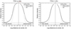 |
Fig. 7 Normalized surface brightness profiles of comet C/2011 KP36 (Spacewatch) and a field star (dotted line) measured in the g-sdss and r-sdss images. Profiles are taken across the central region of the comet along jets J1 and J2 located in the solar and antisolar directions (solid line) and jets J3 and J4 located close to perpendicular to the solar-antisolar direction (dashed line). |
Model parameters for different spatial brightness profiles in the g-sdss and r-sdss filters.
7 Characteristics of the nucleus and dust coma
7.1 Nucleus
The only estimates of geometric albedo (pv = 0.101 ± 0.062) and diameter of the nucleus of comet 2011KP36 (D = 55.1 ± 19.4 km) were derived by Bauer et al. (2013) from the Wide-field Infrared Survey Explorer (WISE) observations in the thermal infrared range and subsequent modeling. The absolute magnitude of the comet (Hv (1,1,0) = 9.4m ± 0.3m) based on discovery and astrometric observations was provided by the Minor Planet Center (MPC)2.
Taking into account the contribution of the nucleus to the integral intensity of the coma, we have estimated the nucleus magnitude in the g-sdss filter, mg = 17.29m ± 0.26m, and in the r-sdss filter, mr = 15.93m ± 0.15m. Thus, the derived color, g – r = 1.36m ± 0.30m, shows that the nucleus of comet 2011KP36 is very red. Given the error in mg, the nucleus color may be in the range 1.0m–1.7m within 1σ. The error in mg is quite large, which may be caused by a small contribution of the nucleus and, perhaps, the molecular emission component to the g-sdss image, as well as by the rather strong asymmetry of the coma. Since the ratio of cometary spectrum to the Solar spectrum increases by 20% in the red range, the color should have a noticeable positive excess. Therefore, we concluded that the nucleus color of comet 2011KP36 most likely has a value closer to the lower limit of the permissible values, between 1.0m and 1.4m.
Classification of comets and related bodies according to their colors in the B, V, and R photometric bands was carried out by Jewitt (2015). To compare our results with those of Jewitt, we need to convert the g – r color in the SDSS photometric system to the B – R color in the Johnson–Cousins system. We used the obtained spectrum of comet 2011KP36 and the transmission curves corrected for the CCD sensitivity in the g-sdss, r-sdss, B, and R filters that were taken from the website3 of the 6-m BTA telescope of the SAO RAS. We convolved the cometary spectrum within the transmission curves for each filter. Correction coefficients to convert magnitude from the SDSS system to the Johnson-Cousins system for comet 2011KP36 were calculated using the ratio of fluxes in pairs of filters from different photometric systems. As a result, the color of the cometary coma in the SDSS photometric system is g–r = 0.65m ± 0.07m (see Table 7), which corresponds to B – R = 1.22m in the Johnson–Cousins system. The color of the cometary nucleus in the Johnson–Cousins system is B – R = 1.9m ± 0.3m, confirming that the nucleus of comet 2011KP36 is ultrared.
In his paper, Jewitt (2015) noted that the colors of the nucleus and the dust coma of a given object can be intrinsically different, or the difference can be caused by the change of the particles with time since release from the nucleus. Moreover, Jewitt showed that the mean optical colors of the dust in short-period and long-period comets are identical within the uncertainties of measurement and there is no evidence for ultrared matter. We compared the obtained color of the nucleus of comet 2011KP36, but not the color of the cometary coma, with the data (median or mean B – R color) presented in Table 10 from Jewitt (2015). It turned out that the B – R color of the nucleus of comet 2011KP36 is close within the measurement error to the colors of Kuiper belt objects (1.5m–1.7m).
To estimate the diameter of the cometary nucleus, we used the nucleus magnitude in the r-sdss filter, since it is more accurate. This value was corrected for the Sun and Earth distances of the comet, and we derived the absolute magnitude of the comet, Hr (1,1,0) = 9.15m ± 0.15m. Using the color of the Sun, we transformed the value Hr in the r-sdss filter to the absolute value HV in the filter V and obtained HV = 9.43m ± 0.15m. Assuming the same geometric albedo of 0.101 ± 0.062 obtained for 2011KP36 by Bauer et al. (2013) and taking into account the spectral gradient of reflectivity, we have estimated the diameter of the nucleus of comet 2011KP36 to be D = 47.3 ± 17.5 km. Here, the error includes both the albedo error and the absolute magnitude error. The obtained values of the absolute magnitude and diameter are consistent with those (HV = 9.4m, D = 55.1 km) obtained by Bauer et al.
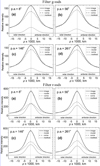 |
Fig. 8 Modeled and observed brightness profiles in comet C/2011 KP36 (Spacewatch) in the g-sdss and r-sdss filters along the directions with the position angles of 8° (jet J4, plot a), 56° (coma C1, plot b), 146° (coma C2, plot c), and 261° (jet J1, plot d). The observed and modeled profiles are designated by a black solid line and a dotted line, respectively. The coma profile is shown by a dashed line, and the calculated profile for the comet nucleus by a gray solid line. Negative distance is in the solar direction, and positive distance is in the antisolar direction. |
Characteristics of the dust coma of comet C/2011 KP36 (Spacewatch) determined by different methods.
7.2 Dust coma
Using photometric images of comet 2011KP36, we calculated the integrated magnitudes of the coma in the g-sdss and r-sdss spectral bands, and then g–r color for the comet. The coma magnitude was measured in a circular aperture centered on the central brightness peak defined by the isophots. The aperture radius was 7′′, which corresponds to 22 694 km on the comet. The cometary magnitude was calculated by the expression
![Mathematical equation: \begin{equation*}m_{\textrm{c}}=-2.5\log \left[\frac{I_{\textrm{c}} (\lambda)}{I_{\textrm{s}} (\lambda)} \right] + m_{\textrm{s}} - 2.5\log\,p(\lambda)\Delta M,\end{equation*}](/articles/aa/full_html/2021/07/aa39668-20/aa39668-20-eq8.png) (6)
(6)
where mc is the apparent magnitude of the comet calculated for the aperture of radius ρ, Ic and Is are the measured fluxes of the comet and the standard star in counts, respectively, ms is the standard star magnitude, p(λ) is the sky transparency that depends on the wavelength, and ΔM is the difference between the airmass of the comet and star. The apparent magnitudes of comet 2011KP36 obtained in the g-sdss and r-sdss filters and theirs errors are given in Table 7.
We used the obtained magnitudes of comet 2011KP36 to calculate the parameter Afρ that characterizes the relative dust production rate (A’Hearn et al. 1984). For the calculation of the quantity Afρ, we used the formula proposed by Mazzotta Epifani et al. (2010):
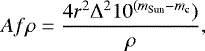 (7)
(7)
where A is the albedo of the cometary dust grains, f is the filling factor in the aperture equal to the fraction of area covered by the dust, ρ is the aperture radius at the comet measured in centimeters, and mSun is the magnitude of the Sun. The heliocentric distance r is in astronomical units and the geocentric distance Δ is in centimeters. For measurements, we chose the aperture radius ρ = 7′′. The obtained Afρ values are 1065 ± 11 cm for g-sdss and 1264 ± 17 cm for the r-sdss filters. In Table 7, we present our results together with the results derived by Sárneczky et al. (2016) and Garcia et al. (2020) in the pre-perihelion period of comet 2011KP36. Comparison of the Afρ parameter for comet 2011KP36 before and after perihelion passage shows that the Afρ value obtained by Garcia et al. (2020) before perihelion (313 days) at r = 5.38 au is 4444 cm, while our observations at almost the same heliocentric distance, r = 5.06 au, but after perihelion (183 days), give an average value Afρ ≈ 1164 cm, which is approximately four times lower. Although the comet was at similar heliocentric distances, the interval between these observations was more than 16 months. It is natural to assume that during this time some nonstationary processes (e.g., outbursts, seasonal effects, or perhaps both) occurred in the comet4, which could significantly change the dust production rate.
One of the characteristics of dust is the normalized gradient of reflectivity, which can be calculated from the photometric data as follows (Jewitt & Meech 1986):
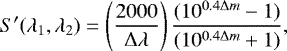 (8)
(8)
where S′ is the normalized gradient of reflectivity in percent per 1000 Å, Δλ = λ2–λ1 is the difference in the effective wavelengths of the g-sdss (λ4650/1300 Å) and r-sdss (λ6200/1200 Å) filters, and Δm is the difference between the comet color and the Sun color. The obtained S′ value of the reflectivity gradient for comet 2011KP36 is given in Table 7.
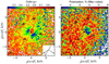 |
Fig. 9 g – r color map (left panel) and polarization map in the r-sdss filter (right panel) of comet C/2011 KP36 (Spacewatch) observed on November 25, 2016 at the phase angle 9.6°. Corresponding scale bars in magnitude for the color map and in percentage for the polarization map are displayed at the top of the images. The location of the optocenter is marked by a black cross, jets by black lines, and the possible shell and arcs are indicated by white dotted lines. The arrows point in the direction to the Sun (⊙), north (N), east (E), and the negative velocity vector of the comet as seen in the observer’s plane of sky (V). Negative distance is in the solar direction, and positive distance is in the antisolar direction. |
8 Distribution of color and polarization over the coma
From the observations of comet 2011KP36 in two different filters, g-sdss (λ4650/1300 Å) and r-sdss (λ6200/1200 Å), we were ableto create a g – r color map to search for small-scale features in the coma and in the detected jets. Using the central brightness peak in the coma defined from the isophots with an accuracy of 0.05 px, the flux calibrated images of the comet in both bands were carefully centered on the same position and added each set of images together. After this, we converted each pixel in the summed images into the apparent magnitude and created the final g – r color map by subtracting the two sets of images from each other (Fig. 9a, left panel). An average error in the magnitude measurements is 0.03m. From the color map, one can see that the dust color in the coma area of about 10 000 km is very red; on average the color index is ~0.8m near the optocenter. There are two areas of blue color (~0.2m) on both sides of the nucleus, approximately along jets J3 and J4.
The distribution of the degree of linear polarization over the coma in the r-sdss filter is shown in Fig. 9b (right panel). In all areas of the coma, the polarization degree is negative, which means that the plane of polarization is parallel to the scattering plane. The figure shows that there is a complex structure of the coma in polarized light, with areas of high and low polarization, indicating the presence of different dust particles. A region of higher negative polarization, approximately –5%, is seen in the innermost coma, up to distances of about 3000–8000 km, depending on the direction. There is also an area of low polarization, –(1–2)%, which is located between jets J2 and J4. It seems to us that there are also several structural features with a higher polarization. There is a shell with the polarization degree –(4–6)% located in the antisolar direction at distances of approximately 24 000 km to 43 000 km from the optocenter. Besides, there are two almost parallel arcs with the higher –(5–6)%) polarization at distances of about 35 000 and 53 000 km in the solar direction.
Comparison of the color and polarization maps in Fig. 9 shows that there is no unambiguous relationship between the changes of color and the degree of polarization. The near-nuclear region is characterized by a high degree of polarization and red color. The color in the coma region with low polarization –(1–2)% varies from 0.2m to 0.7m. The shell in the antisolar direction is characterized by a high degree of polarization –(5–6)% and significant color changes, from 0.2m to 0.6m. Such a complex relationship between color and polarization indicates dust particles of various compositions and sizes released from the surface and active areas of the cometary nucleus. According to our measurements, the integrated degree of polarization measured with a circular aperture is practically independent from the aperture radius within the error limits.
The map of the polarization vectors in the coma presented by the position angles of the polarization plane is shown in Fig. 10. These polarization angles are measured within the coma area of 10 000 × 10 000 km2. The orientation of the vectors indicates the direction of the local polarization plane, and their length indicates the degree of polarization. In general, the polarization vectors have been found almost parallel to the scattering plane. The mean value of the position angle in the coma is about 62 ± 6°, and the polarization plane is parallel to the scattering plane (φ = 61.49°). Although Fig. 10 demonstrates some deviations, reaching 3°–4°, they are within the limits of the 1σ uncertainty.
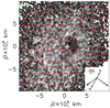 |
Fig. 10 Distribution of the polarization vectors in the coma of comet C/2011 KP36 (Spacewatch). The orientation of the vectors indicates the direction of the local polarization plane, and the length of the vectors marks the degree of polarization. The arrows point in the direction to the Sun (⊙), north (N), east (E), and the negative velocity vector of the comet as seen in the sky plane (V). Negative distance is in the solar direction, and positive distance is in the antisolar direction. |
9 Spatialvariations of color and polarization
9.1 Profiles of color and polarization
Digital processing of the images of comet 2011KP36 revealed four jet-like structures in the coma (see Fig. 3). To investigate whether there are any polarimetric and color trends along these jets, we have taken scans from the photometric center of the comet along the J1, J2, J3, and J4 jets. Additionally, the cuts were made through the coma in the directions between the J4 and J2 jets (PA = 56°, the antisolar direction) and J3 and J1 (PA = 236°, the solar direction). For this, we estimated the observed color and polarization with a 3 × 3 px size aperture (or 3501 × 3501 km at the comet), starting from the photometric center of the comet.
Figure 11 (top panel) shows the cuts across the g – r color map. In the near-nucleus region, the color index is about 0.7m. At distances around 12 000 km from the photocenter, the dust color sharply drops to ~0.3m. Starting from these distances, the g – r color index of the dust slightly increases along the jets and the coma with increasing distance from the nucleus, especially in the solar direction, suggesting some evolution of the dust particles.
As was shown in Sect. 7.1, the nucleus of comet 2011KP36 is large and very red. The contribution of the nucleus brightness to the brightness profiles in the g-sdss and r-sdss filters was shown in Fig. 8. Based on the profiles shown in this figure, we accounted for the contribution of the nucleus color to the coma color profiles. The radial profiles of the dust color without the nucleus contribution along the measured directions are presented in Fig. 11. Corrected for the contribution of the nucleus, the color index g – r decreases sharply from about 0.7m in the innermost near-nucleus coma to on average ~ 0.4m. The figure (top panel) also shows that the nucleus affects the color profiles to a distance of about 15 000 km. From this distance, the nucleus does not affect the color of the dust.
The observed radial profiles of polarization across the jet structures and the coma are shown in Fig. 11 (bottom panel). On the average, in the near-nucleus coma, the maximum (negative) polarization is –5.2%. In the first quadrant, there is an area (blue color in polarization map, Fig. 9 b) with the minimum degree of polarization, – (1–1.8)%, within the range of distances 8000–15 000 km. Between 25 000 km and 40 000 km, a shell with an average degree of polarization of about –4% is observed. Furthermore, with increasing distance up to ~ 90 000 km in the antisolar direction, the polarization degree varies between –1% and –4%, depending on the direction. In the solar direction, the degree of polarization slightly increases (in absolute value) with wave-like variations up to –(2–5)%. Also, there are arcs in which the polarization increased up to –5.2%.
The observed degree of polarization is a combination of the polarization of the dust coma and the nucleus. To the best of our knowledge, polarization of cometary nuclei has only been measured so far for comet 2P/Encke (Boehnhardt et al. 2008) and the main-belt comet 133P/Elst-Pizarro (Bagnulo et al. 2010). In these cases, the polarization appeared to be –0.85% and –1.4% at the phase angle α = 10°. According to Bagnulo et al. (2017), the phase-angle dependence of polarization of the cometary nucleus is similar to that for F-type asteroids. Thus, the polarization of the nucleus of 2011KP36 most likely is lower than the observed polarization in the near-nucleus area of the coma and should be taken into account when calculating the polarization of the cometary dust.
Taking into account the contribution of the nucleus to the integral intensity of the coma (Sect. 7.1, Fig. 8), we evaluated the nucleus input in the polarization of the dust coma. For this, we used the ratio of fluxes k(ρ) = Fnucl(ρ)∕Fdust coma(ρ) in the cuts along jets J1, J2, J3, and J4, and the cuts through the coma in the antisolar (PA = 56°) and solar (PA = 236°) directions inthe r-sdss filter. Computation of the dust coma polarization free from the nucleus polarization was performed according tothe expression
 (9)
(9)
where Pobs(ρ) is the observed polarization along the cuts, and Pnucl is the polarization of the nucleus. The detailed derivation of this equation is presented by Kiselev et al. (2020). We assumed that the polarization of the cometary nucleus is close to the averaged polarization for nuclei of 2P/Encke (Boehnhardt et al. 2008) and 133P/Elst-Pizarro (Bagnulo et al. 2010); Pnucl = –(1.2 ± 0.17)% at the phase angle 10°. Using the technique described by Kiselev et al. (2020), we estimated the uncertainty in the coma polarization after correction for the nucleus contribution; the maximum absolute error is ΔPdust coma ≈ 1%. Figure 11 (bottom panel, red lines) shows the variations of the dust coma polarization with distance from the nucleus after removing the nucleus contribution. Within the innermost area of the coma, polarization of the dust coma after removing the nucleus contribution is approximately –7 ± 1%, while the observed polarization is –5.2 ± 0.2%. At the distances larger than ~8000 km from the optocenter of the coma, the contribution of the nucleus polarization to the coma polarization is negligible.
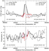 |
Fig. 11 Radial profiles across the g – r color (top panel) and polarization (bottom panel) maps of comet C/2011 KP36 (Spacewatch). The individual curves are scans measured from the photometric center of the comet through the J1, J2, J3, and J4 jets and the coma in different directions: the solid black line is the cuts along the J1and J2; the dotted line is the cuts along the J3 and J4; the solid gray line is the cuts across the nucleus and coma in the directions with PA = 56° and PA = 236°. The radial profiles of the dust color without the nucleus contribution are marked by colored lines. Zero point is at the photometric center of the comet. Vertical dashed lines show the size of the seeing disc during the observations. Negative distance is in the solar direction, and positive distance is in the antisolar direction. |
9.2 Fourier analysis of spatial variations of color
An active area on the nucleus, rotating in and out of sunlight, would drive a variable outflow of matter that would appear in the coma as time-dependent variations in the profiles of brightness, color, and polarization. We carried out a Fourier analysis of the spatial variations in color and polarization along jets J1 and J2. For this, we took into account the spatial location of the investigated jets and the projection conditions of the jets onto the sky plane. In jets J3 and J4, we see a substance on the line of sight ejected at different times. Therefore, the spatial frequencies for these jets are determined unreliably. In the case of color, the spatial frequency spectra for the profiles of independent jets J1 and J2 are similar in the region up to 1 × 10⁴ km−1 where the most significant components are located (Fig. 12a). This provides evidence for the fact that color index fluctuations for these profiles should be caused by a single factor, namely, the rotation of the nucleus. The main components of spatial frequencies are shown in Table 8. The table shows the amplitudes, frequencies, and distances in the jet structures that correspond to a given spatial frequency. Since the angle between the geocentric vector of the comet and the rotation axis of the nucleus is about 75°, the indicated distance corresponds to the spatial distance in jets J1 and J2. There is a frequency of 7.5 × 10⁻⁵ km−1 for the J1 jet corresponding to a characteristic length of 1.33 × 10⁴ km, which is equal to the product of the rotation period of the nucleus and the velocity of the matter outflow. This spatial frequency is also present in the amplitude spectrum for the J2 jet, but its amplitude is lower than the 2.5σ level, therefore we cannot draw reliable conclusions about its existence. The same value ((1.33 ± 0.12) × 104 km) is also determined from the geometric model of jets (see Sect. 4.2).
The second important peak in the spatial frequency spectrum is apparently related to the precession of the nucleus. The characteristic periods 3.07 × 10⁴ km for the J1 jet and 3.22 × 10⁴ km for the J2 jet are close to the period of the wave structure of the J4 jet. Small dissimilarities in the values of the periods may be explained by both possible errors and differences in the velocities of matter ejections from different active areas. The other peaks in thefrequency spectrum are explained by combinations of basic frequencies related to the nucleus rotation (fr) and precession (fp). For the J1 jet: 0.5fp = 1.63 × 10⁻⁵ km−1, 2fp = 6.52 × 10⁻⁵ km−1, fr –fp = 4.23 × 10⁻⁵ km−1 ≈ 4.56 × 10⁻⁵ km−1 and for the J2 jet: 0.5fp = 1.55 × 10⁻⁵ km−1 ≈ 1.81 × 10⁻⁵ km−1, fr –fp = 4.40 × 10⁻⁵ km−1 ≈ 4.65 × 10⁻⁵ km−1. Comparing the frequencies, it is necessary to take into account that the spatial frequency sampling step is approximately equal to 0.4 × 10⁻⁵ km−1.
Another approach can be used to analyze the J3 and J4 jets. The spatial color profiles of these jets should be influenced by the nucleus precession. Since the J4 jet forms when the active region comes out of the shadow,a lag in the J3 pattern by about half the period should be observed. Indeed, the maximum correlation between the spatial color profiles of jets J3 and J4 is observed when the J3 profile is shifted by +1.49 × 10⁴ km. However, in this case, it is necessary to take into account the difference in characteristic scales of the spatial profiles. For the J3 jet, the distance between the peaks is 1.1 times larger than between the corresponding peaks for the J4 jet. This could be explained by the fact that the J4 jet was formed by a cold area that had just left the shadow, while J3 was formed by a heated area before it entered the shadow. Presumably, the outflow velocity of gas and, accordingly, dust will be greater for the heated region. As a result, the characteristic scale for the J3 jet may be larger than in the observed profiles. The correlation coefficient for profiles outside the near-nucleus regions, taking into account the shift and the difference in scales, reaches 0.65, which may indicate a nonrandom nature of such behavior.
Figure 12 b shows the spatial g – r color profiles for jets J3 and J4, however, for the J3 jet profile, the distance scale is 1.1 times smaller and the shift is 1.49 × 10⁴ km. Since this shift corresponds to half the precession period, the precession scale, determined from the shift of the J3 and J4 jet scales, is 2.98 × 10⁴ km. This value is in good agreement with the values determined from the Fourier analysis of the color profiles for jets J1 and J2 and the wave structure in jet J4. We can conclude that the characteristic scale of the precession is (3.0 ± 0.15) × 104 km and the ratio of the periods of the precession and nucleus rotation is 2.26 ± 0.20.
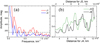 |
Fig. 12 (a) Single-sided amplitude spectrum of the spatial frequencies of color profiles for jets J1 and J2 in comet C/2011 KP36 (Spacewatch) observed on November 25, 2016. (b) Comparison of the spatial color profiles forthe J3 and J4 jets with different distance scales from the nucleus of the comet to demonstrate the correlation between the profiles. The dashed line shows the magnitude of the random signal at 2.5σ level. |
Main components of the spatial frequencies in color profiles for jets J1 and J2.
10 Characteristics of the coma dust particles from numerical modeling
This section describes our attempt to model the physical characteristics of the dust particles in the coma of 2011KP36 based on the approach we successfully used in Ivanova et al. (2019). As in Ivanova et al., we presented the dust particles as an ensemble of rough spheroids with a log-normal size distribution of particles, described by the effective radius, reff, and the effective variance veff = 0.1. The axes ratios of the spheroids ranged from –3 to 3 (i.e., the mixture included both prolate and oblate spheroids). The size of the spheroids was defined through the radius of a sphere of equal volume; we considered reff for a variety of values from 0.1 to 10 μm. Roughness was presented by a normal distribution of the spheroid surface slopes, defined by the standard deviation of the slope distribution taken to be equal to 0.2 in this study (for more detail, see Kolokolova et al. 2015). In our modeling, we took advantage of the library of pre-calculated kernels for computations of the light scattering characteristics of rough spheroids (Dubovik et al. 2006), which allowed us to quickly obtain brightness and polarization for a variety of dust compositions, size distributions, and spheroid shapes.
Our modeling included the following materials: silicates (forsterite), water ice (solid and porous), CO2 ice, tholin, ice tholin, Halley dust (a mixture of silicates, organics, and carbon that fits the in situ characteristics of the dust in comet Halley, see Kimura et al. 2003), considered as solid and of different porosity, and an intimate mixture of ice and Halley dust. The refractive indices of pure materials are listed in Ivanova et al. (2019). For the intimate mixtures and porous materials, we used the Maxwell Garnett mixing rule to determine the effective refractive index.
Following the approach described in Ivanova et al. (2019), we performed a survey of the polarization and color characteristics of dust of different compositions and particle size and their mixtures, trying to fit not only specific values of color and polarization but also to reproduce their trends in the coma. Unlike the case of comet C/2014 A4 (SONEAR) studied in Ivanova et al., where we observed very red color (about 0.8m) and an extremely high value of negative polarization, reaching –8% at the phase angle about 4°, in the case of 2011KP36, after the effects of the nucleus had been subtracted, the values of color and polarization were more regular. The color index stayed around 0.4m, which is typical for comets (Jewitt 2015), and the highest value of the negative polarization did not exceed –5%. This is rather high in comparison with regular comets, however, as was shown in Ivanova et al. (2019), at phase angles of 10°, this value can be reached if the dust represents a rather typical mixture of porous Halley dust particles with solid silicate particles (Kolokolova & Kimura 2010). To correctly characterize the particles in the 2011KP36 coma, we modeled not just specific values of color and polarization, but also the trends in their change in the coma. The modeling was done for all scansshown in Fig. 11, namely, for J1, J2, J3, J4, and the directions in the coma with PA = 56° and PA = 236°. We also separately modeled unusual features in the maps shown in Fig. 9: a blue color in the directions of J3 and J4, and an area of low polarization in the quadrant between J2 and J4.
Our modeling showed that a single material cannot describe the behavior of color and polarization in any direction in the coma. To fit the observed data, we had to use a mixture of two materials, and this was done by modeling all combinations of any two materials listed above, considering mixtures of all their sizes and combining them in different proportions from 1:9 to 9:1.
Among all the results we selected those that represented the combination of the observed values of color and polarization near the nucleus and far from the nucleus (at a distance of about 75 000 km). For the ‘blue’ features, we considered the values of the color and polarization at the maximum of the feature and at the distance where the values returned to regular ones.
Our modeling ended up with more than 20 different solutions for each direction. To select the realistic cases among them, we took into consideration the following conditions:
With distance from the nucleus, particles can become only smaller as a result of evaporation of volatile materials or/and fragmentation of particles;
The size of particles made of more volatile materials (i.e., CO2) diminishes faster than that of particles made of less volatile materials (e.g., water ice);
No material that was not present near the nucleus can appear at larger distances;
The ratio of different materials in the mixture should change in accordance with the change in particle size. For example, if the size of the particles does not change, the ratio should not change either. If refractory particles become smaller, which can result only from fragmentation, then the abundance of those particles (number density) should increase, changing the ratio correspondingly;
The results in different directions should be consistent. Therefore if among the numerous fitting combinations of materials we found that a specific combination of materials, for example, silicate and tholin, reproduced the data in one direction in the coma but not in any other, we excluded it from consideration.
The most consistent model of the dust in the different directions in the observed coma of 2011KP36 is presented in Table 9. The values of the color and polarization in the table show the median values from the range of values we considered. To account for the large oscillations in the values, we considered all values of color within ± 0.05m from the median value and all values of polarization within 0.5% from the median value for large distances from the nucleus. “HD+ice, 90%” in the table means an intimate mixture of Halley dust and water ice, with 90% of Halley dust in the mixture; from now on, we call the particles of this composition “icy Halley dust particles”.
Due to a large uncertainty in color and polarization caused by the oscillations, we have found other solutions, for slightly different sizes of particles, which provided a reasonable fit to the observations. Table 9 presents only one of them that fits the specific values of color and polarization shown in Cols. 2 and 3. However, all the good-fit solutions have the following in common:
The effective radius of the dust particles is in micron range;
A mixture of icy Halley dust particles with water ice is a dominant component of the coma;
The presence of CO2 ice is required to explain low polarization in the quadrant 0–90° and changes in color and polarization with the distance from the nucleus in this area.
Thus, the size of particles in Table 8 is not unique, but the composition of particles is determined quite reliably. Specifically, no other composition except a combination of CO2 ice and water ice could explain the observed combination of color and polarization and their trend with the distance from the nucleus in the quadrant between jets J2 and J4. On the other hand, no results that would include CO2 ice were found for the quadrant between J1 and J3, where a mixture of icy Halley dust particles and pure water ice particles were required to fit the observations.
Based on our modeling, we can assume that the low polarization area in the quadrant between J2 and J4 is caused by the ejection of a cloud of CO2 and water ice particles (outburst?). The rest of the coma is formed by water ice and icy Halley dust particles; this may indicate that these particles are more typical for the 2011KP36 nucleus.
We do not want to speculate what causes color and polarization oscillations in the coma, especially because they do not show any regularities: some increases in color correlate with increases in polarization, some of them anticorrelate, and the majority of them do notshow any type of correlation. This indicates that a variety of dust properties are responsible for those oscillations. Based on our modeling and general physical principles, we may assume that areas of less negative polarization indicate the presence of smaller particles or a smaller abundance of transparent (e.g., water ice) particles, and the areas of bluer color indicate either the presence of smaller particles or a larger abundance of water ice. In the wavelength range between g-sdss and r-sdss filters, which is between 4 650 Å and 6 200 Å, the imaginary part of the refractive index of water ice experiences a ten-fold increase, whereas for CO2 ice it only doubles (see Ivanova et al. 2019). Therefore, it is more likely that changes in color are caused by changes in the water ice abundance than in the CO2 abundance.
11 Discussion and conclusions
We present the results of an analysis of quasi-simultaneous spectroscopic, photometric, and polarimetric observations of the long-periodic (perihelion is q = 4.88 au) comet C/2011 KP36 (Spacewatch) derived at the 6-m telescope BTA of the SAO RAS. The main conclusions from this study are summarized below.
Spectra
The spectrum of comet 2011KP36 exhibits the presence of quite strong emission bands of the ion CO+, but there are no emissions of the typical cometary molecules CN, C3, and C2, and also N (Fig. 2). The reflectivity gradient (about 12% per 1000 Å) obtained over the wavelength range 4650–6200 Å (Fig. 1) differs significantly from those obtained for comets of the Jupiter family. According to Storrs et al. (1992), a mean value of about 22% per 1000 Å was found within the group of 18 ecliptic comets, with minimum and maximum values of 15% per 1000 Å and 37% per 1000 Å, respectively. Houpis & Mendis (1981a,b) showed that a CO or CO2-dominated surface of the cometary nucleus could explain not only the strong coma and tail activity at large heliocentric distances, but also the irregular activity of such comets at these distances. Comet 2011KP36 exhibits conspicuous activity at r > 5 au and emission bands of CO+. According to Womack et al. (2017), CO is difficult to photoionize beyond 5 au from the Sun, so detecting emissions of CO+ implies either an unusual ionization mechanism of CO or, more likely, a very large amount of CO in the coma. On the other hand, Ivanova et al. (2019) showed that for the CO-rich comet 29P/Schwassmann-Wachmann 1 (Gunnarsson 2003; Paganini et al. 2013), impact ionization by Solar wind particles is the main ionization mechanism at large heliocentric distances (more 5 au). This mechanism may also be applied to comet 2011KP36.
Composition and size of the dust particles in different directions in the coma of comet C/2011 KP36 (Spacewatch) modeled with the rough spheroid model.
Morphology
By applying different enhancement techniques to the original images of comet 2011KP36 in the g-sdss and r-sdssfiltersto make the faint coma visible, we have revealed four jet-like dust structures that are designated as J1 (PA = 261°), J2 (103°), J3 (188°), and J4 (8°) (Fig. 3). To explain these structural features in the coma, we modeled the continuous flow of dust particles from three discrete active areas using a geometrical model of jets (see Appendix A) and obtained the following results:
The projected rotation axis of the nucleus is located along the direction J1–J2 and lies nearly in the picture plane (an inclination of approximately 15°). The coordinates of the north pole of rotation axis are the following: right ascension RA = +280° and declination Dec = –60°.
-
Source 1, which forms the sunward-facing jet J1, is located on the illuminated north hemisphere of the nucleus at the cometocentric latitude φ = +78°. Jet J2 originates from active Source 2 and is located in the south hemisphere at latitude φ = –75° in the transition region between the night and day side of the nucleus, balancing between shadow and light during a significant part of the rotational period. The rotation of the nucleus leads to the formation of a cone of ejected material from Source 1, as well as from Source 2 in the solar and antisolar directions (Figs. 4 and 5). Our conclusion is supported by the data of Garcia et al. (2020), which indicate a morphology resembling corkscrews that transform into conical structures with increasing distance from the nucleus. According to Sekanina (1979), such a cone may be produced when a high-latitude source on the Sun-facing hemisphere is carried around the rotational pole. The axis of this cone slightly deviates from the sunward direction (about 19° for J1) and is shifted toward the projection of the rotation axis on the sky plane (Fig. 4). When the jets rotate, they form cone-like structures, with a change in brightness modulated by the rotation of the nucleus. This explains the quasi-periodic fluctuations in color (Fig. 11).
Two visible jets J3 and J4 are formed by a single active area (Source 3) on the surface, located near the equator of the cometary nucleus, φ = –5°. Considering the orientation of the nucleus rotation, it is evident that jets J3 and J4 form a ring around the nucleus over several revolutions of the nucleus, which we observe edge-on as the jets projected to the left and right of the nucleus. This phenomenon is demonstrated in Figs. 4 and 5. The lower activity of Source 3 compared to the other two active areas, located in the polar zones, may be explained by local features of the cometary nucleus.
Brightness profiles
We found that the radial profiles of the surface brightness of the dust coma in comet 2011KP36 (Fig. 6) are significantly less steep than the canonical 1/ρ for projected radial distance within the range of approximately 5000–20 000 km. The power index n was substantially smaller than unity and varied between 0.55 and 0.80. Moreover, spatial profiles of brightness showed a distinct asymmetry in the solar-antisolar direction, namely, there is a slight systematic difference in n for the sunward(J1 and J3 jets and sunward coma) and antisolar (J2, J4, and antisunward coma) directions. These effects may be caused by anisotropies in the dust ejection from the nucleus, resulting in a deviation from the spherical symmetry of the coma, or nonsteady activity (i.e., outbursts), which is characteristic for this comet. The dust in the sunward jets and the coma ejected from the sunward-facing surface of the nucleus had either a slightly different size distribution of the dust particles, or a slightly different velocity compared to the antisolar side.
In most comets, the surface brightness profiles are characterized by a slope with a power index n equal to or greater than 1. Jewitt & Meech (1987) concluded that several processes, including SRP, the sublimation of ice grains, and variable mass loss from the nucleus, may all give rise to coma profiles with gradients different from n = 1. Rather flat brightness profiles were observed previously in comet Encke (Sekanina & Schuster 1978; Djorgovski & Spinrad 1985; Rosenbush et al. 2020). The explanation for this (see also O’Dell et al. 1988) could be either the fragmentation of particles or an increase in their albedo, or the deceleration of particles with distance from the nucleus. Our modeling of the color and polarization distribution revealed neither fragmentation of dust particles nor evaporation of any dark material in the coma of comet 2011KP36. We suggest that the flatness of the brightness profile results not from changes in the particle properties as they move through the coma, but from the inhomogeneity of the coma, where at different distances from the nucleus we see the particles ejected at different times and from different active areas.
Nucleus and dust coma
Using a value for the geometric albedo of 0.101 ± 0.062 obtained for comet 2011KP36 by Bauer et al. (2013), we estimated the nucleus diameter to be D = 47.3 ± 17.5 km. We also used the method by Harris & Harris (1997) to approximate the object diameter and derived a D of about 45 km. The obtained values of the absolute magnitude and diameter are consistent with those (HV = 9.4m, D = 55.1 km) obtained by Bauer et al. (2013). However, if we accept a lower geometric albedo, for example, 0.08, which is the collective mean for the populations of Centaurs and SDOs as a whole (Bauer et al. 2013), we obtain a larger diameter, 53.1 ± 3.8 km, where the error includes only the absolute magnitude error. Thus, comet 2011KP36 apparently has the largest nucleus among the known comets.
The obtained values of the parameter Afρ, which characterizes the relative dust production rate in the comet, equal to 1065 ± 11 cm for the g-sdss and 1264 ± 17 cm for r-sdss filters, are typical for the distant comets (Storrs et al. 1992; Korsun et al. 2016; Kulyk et al. 2018; Ivanova et al. 2019). However, the reflectivity gradient of the dust coma of comet 2011KP36 (about 12% per 1000 Å) differs significantly from that obtained for comets of the Jupiter family and is close to the average value typical for the most distant comets (Storrs et al. 1992; Korsun et al. 2016; Kulyk et al. 2018; Ivanova et al. 2019).
We estimated the contribution of the nucleus to the integral intensity of the coma and based on this obtained the g – r color of the cometary nucleus, which appeared to be 1.4m ± 0.3m corresponding to B – R = 1.9m ± 0.3m; thus, the color of the nucleus of comet 2011KP36 is ultrared. Using a classification suggested by Jewitt (2015), comet 2011KP36 may be attributed to the Kuiper belt objects (their mean B – R colors ranged within 1.5m–1.7m).
There are many explanations for the ultrared color of the surfaces of distant objects. It is known that complex organic molecules can efficiently absorb optical light at shorter wavelengths, which can lead to a reddening of the object (Peixinho et al. 2020), although other compounds are capable of doing this too. For example, Brown et al. (2011) and Wong & Brown (2016) argue in favor of H2 S as the main reddening agent, rather than organic molecules. If the object is located beyond the H2 S sublimation line, thus are not depleted of H2S, it would experience radiation reddening. On the other hand, Kaňuchová et al. (2012) showed that it was possible to reproduce the whole range of colors observed on the outer Solar System small bodies with an appropriate combination of initial albedo, space weathering, and meteoritic bombardment. However, there is no evidence for ultrared matter in the small body populations in the inner Solar System. Jewitt (2015) presumed that in the process of evolution of an object, cometary activity can expose the inner neutral or blue material and leads to the disappearance of ultrared matter. Since the comet’s nucleus has an ultrared color, it is likely that comet 2011KP36 was relatively recently ejected from the Kuiper belt to the inner part of the Solar System. Accordingly, the activity of the nucleus has not yet had time to change its color to more neutral or blue.
Spatial variations of color and polarization
The observed color and polarization maps show a complex structure of the coma, however, the relationship between the changes of color and the degree of polarization is ambiguous. In the innermost coma (to distances of about 3000–15 000 km, depending on the direction), the dust is red (on average g–r ≈ 0.6–0.7m) and has a high negative polarization, approximately –5% at the phase angle 9.6°. After taking into account the nucleus contribution, the color in the near-nucleus area became 0.35m–0.45m, and the polarization degree varied from –1.5% to –4.5%. Farther from the nucleus, there are two areas of blue color (~ 0.2m) on both sides of the nucleus, approximately along jets J3 and J4, and an area of low polarization, –(1–2)%, which is located between jetsJ2 and J4. There are also several structural features with a higher polarization: a shell with a polarization degree of –(4–6)% located in the antisolar direction at distances of 24 000–43 000 km from the optocenter and two almost parallel arcs with a higher – (5–6)% polarization at distances of about 35 000 and 53 000 km in the solar direction.
In general, there is a certain correlation between the observed trends in color and polarization degree: an increase in color and polarization is observed with the distance from the nucleus; almost constant color and polarization are seen in jet J2, starting from approximately 30 000 km, while in other antisolar directions they slightly increase. In the solar direction, color and polarization increase with increasing distance from the optocenter of the comet. The inhomogeneity of the coma in color and, especially, polarization degree most likely is caused by the activity of different sources of dust on the nucleus, thus indicating inhomogeneity of the nucleus; the variations with the distance from the nucleus in different jets and the coma is a combined effect of temporal variations of the nucleus activity and changes in the dust particle properties on their way out of the nucleus.
Characteristics of the coma dust particles from numerical modeling
Using our observations of comet 2011KP36, we attempted to model the physical characteristics of the dust particles in the coma based on the approach we successfully used in Ivanova et al. (2019). Also in Ivanova et al. (2019), we presented the dust particles as an ensemble of rough spheroids with a log-normal size distribution of particles. Our modeling included the following materials: silicates (forsterite), water ice (solid and porous), CO2 ice, tholin, ice tholin, Halley dust, solid and of different porosity, and intimate mixtures of ice and Halley dust. As a result of modeling, we found that the coma is dominated by water ice and icy Halley dust particles. The low polarization area observed in the quadrant between J2 and J4 jets (see Fig. 9) most likely resulted from an ejection of a cloud of CO2 and water ice particles, which depolarize light due to multiple reflections. At the same time, two large (about 20 000 km) areas of blue color (g – r ≈ 0.2m) corresponding to jets J3 and J4, which represent a single jet “born" by one active area (Source 3), indicate the presence of a larger abundance of fine particles or/and of water ice.
In general, the high variability of the observed characteristics over the coma of comet 2011KP36 indicate significant and variable activity of the nucleus with, probably, numerous small active areas, in addition to the three identified large active areas. Different active areas may release a substance from the nucleus with a different ratio of water ice, CO2 ice, and refractory dust and sizes of their particles, although particles of the size of several microns may dominate in the lifted and ejected material.
Acknowledgements
We thank Alan Fitzsimmons for his thorough review and highly appreciate the comments and suggestions which significantly contributed to improving the quality of the publication. The observations at the 6-m BTA telescope were performed with the financial support of the Ministry of Education and Science of the Russian Federation (agreement No. 14.619.21.0004, project ID RFMEFI61914X0004). The authors express appreciation to the Large Telescope Program Committee of the RAS for the possibility of implementing the program of distant comets at the BTA. The researches by O.I., I.L., V.K., and V.R. are supported, in part, by the project 19BF023-02 of the Taras Shevchenko National University of Kyiv. OI thanks the Slovak Academy of Sciences grant VEGA 2/0023/18. This work was supported by the Slovak Research and Development Agency under the Contract no. APVV-19-0072. IL thanks the SAIA Programme for financial support. The researches by OI, VR, and NK were supported, in part, by the Ukrainian–Slovak joint research project for the period 2017–2019.
Appendix A Geometric method for calculating jet structures in cometary comas
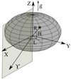 |
Fig. A.1 Coordinate system {XYZ} on the nucleus surface. |
To better understand how the active areas release matter from the nucleus and how the jets are formed, it is necessary to model the geometry of the viewing conditions and the rotation state of the nucleus. For this, we propose a simple geometrical model that takes into account the rotation of the cometary nucleus, the orientation of the nucleus spinaxis, the cometocentric latitude of active areas, and the relative position of the Sun, Earth, and comet. This model suggests that the nucleus is spherical, isolated active area releases gas and dust only under the Sun’s irradiation, and the outflow of matter occurs radially from the nucleus with a constant velocity. Dispersion of the velocities of the particles ejected from the active area and their acceleration under the Sun’s radiation are not considered. As a result, the proposed model allows us quickly to calculate the structure of the jets, select the possible parameters of the observed structures, and trace the formation and change in structural features of the cometary coma. The derived model parameters can be used as a zero approximation for more complex models.
Let us consider a coordinate system {XYZ} associated with the cometary nucleus (Fig. A.1). The Z-axis is directed along the rotation axis of the nucleus. The X-axis lies in the plane that passes through the Z-axis and the direction to the vernal equinox ⋎. The Y-axis complements the XZ-axis to form a right-handed coordinate system. The discrete active source on the nucleus surface is described by spherical coordinates: R is the distance from the nucleus center, L is the longitude measured from the plane passing through the vernal equinox, and B is the latitude. The rotation of the nucleus can be expressed as
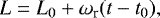 (A.1)
(A.1)
where L0 is the longitude at the initial moment of time t0, t is the current time, and ωr is the angular velocity of the nucleus rotation. The surface of the nucleus is described by the function R(L0, B). Coordinates of the active source in a rectangular coordinate system can be written as
![Mathematical equation: \begin{equation*}\left[\begin{array}{c}x \\y \\z \\\end{array}\right] =\left[\begin{array}{c}R\sin(L_0 + \omega_{\textrm{r}}(t-t_0))\cos B \\R\cos(L_0 + \omega_{\textrm{r}}(t-t_0))\cos B \\R\sin B \\\end{array}\right].\end{equation*}](/articles/aa/full_html/2021/07/aa39668-20/aa39668-20-eq14.png) (A.2)
(A.2)
To account for the precession of the cometary nucleus, let us consider a new coordinate system {X′ Y′ Z′} (Fig. A.2) associated with the parameters of the nucleus precession. The Z′ -axis is directed along the axis around which the precession of the nucleus occurs. The X′ -axis lies in the plane that passes through the Z′-axis and the direction to the vernal equinox ⋎. The Y′-axis complements the right-handed system.
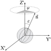 |
Fig. A.2 Coordinate system {X′ Y′ Z′} associated with the precession of the nucleus. |
The orientation of the rotational axis of the nucleus changes due to the precession. The angle of precession ψ is calculated by
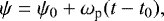 (A.3)
(A.3)
where ψ0 is the precession angle at the initial moment t0, ωp is the angular velocity of the precession, and t is the current time. The components of the unit vector n of the instantaneous angular momentum of nucleus rotation in the reference system {X′ Y′ Z′} are
 (A.4)
(A.4)
where ε is the angular radius of precession. Or, for any vector,
![Mathematical equation: \begin{equation*}\left[\begin{array}{c}x^{\prime} \\y^{\prime} \\z^{\prime} \\\end{array}\right] = rot_z(\varepsilon)rot_y(\psi)\left[\begin{array}{c}x \\y \\z \\\end{array}\right],\end{equation*}](/articles/aa/full_html/2021/07/aa39668-20/aa39668-20-eq17.png) (A.5)
(A.5)
where roty and rotz are the standard rotation matrices around the corresponding axes,
![Mathematical equation: \begin{eqnarray*}rot_y(\gamma) = \left[\begin{array}{ccc}\cos \gamma & 0 & \sin \gamma \\0 & 1 & 0 \\-\sin \gamma & 0 & \cos \gamma \\\end{array}\right],\nonumber \\rot_z(\gamma) = \left[\begin{array}{ccc}\cos \gamma & -\sin \gamma & 0 \\\sin \gamma & \cos \gamma & 0 \\0 & 0 & 1 \\\end{array}\right],\end{eqnarray*}](/articles/aa/full_html/2021/07/aa39668-20/aa39668-20-eq18.png) (A.6)
(A.6)
where γ is an angle of counterclockwise rotation of the coordinate system.
For a j particle that is ejected fromthe k active area with coordinates  , Bk, Rk and with a constant speed Vj at the moment tj, the coordinates in the system {X′ Y′ Z′} for the time t ≥tj are
![Mathematical equation: \begin{eqnarray*}&&\hskip-5pt \left[\begin{array}{c}x^{\prime}_j \\y^{\prime}_j \\z^{\prime}_j \\\end{array}\right] = rot_z(\varepsilon)~rot_y(\psi_0+\omega_{\textrm{p}}(t_j-t_0)) \nonumber \\&& \,{\times}\,\left\{\left[\begin{array}{c}R^k \sin(L_0^k+\omega_{\textrm{r}}(t-t_0))\cos B^k \\R^k \cos(L_0^k+\omega_{\textrm{r}}(t-t_0))\cos B^k \\R^k \sin B^k \\\end{array}\right] + \left[\begin{array}{c}V_{xj} \\V_{yj} \\V_{zj} \\\end{array}\right](t-t_j)\right\}.\end{eqnarray*}](/articles/aa/full_html/2021/07/aa39668-20/aa39668-20-eq20.png) (A.7)
(A.7)
Here Vxj, Vyj, and Vzj are the components of the velocity vector in the reference system {XYZ}, which are chosen so that the velocity vector is perpendicular to the nucleus surface with the k active area. Particle ejection is possible only when the active area is illuminated by the Sun, and then the cosine of the solar zenith distance for the given area must be greater than zero.
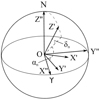 |
Fig. A.3 Transition from the coordinate system {X′ Y′ Z′} associated with the precession of the rotational axis of the nucleus to the equatorial cometocentric coordinate system {X′′ Y′′ Z′′}. |
The coordinates defined in the {X′ Y′ Z′} reference system must be converted to the equatorial coordinate system {X′′ Y′′ Z′′} (Fig. A.3). In this system, the X′′-axis is directed to the vernal equinox ⋎, the Z′′-axis is directed to the celestial pole N, and the Y′′-axis complements the right-handed system. The relationship between the reference system {X′ Y′ Z′} and the equatorial system {X′′ Y′′ Z′′} can be written as
![Mathematical equation: \begin{equation*}\bm{\rho_j}(t)=\left[\begin{array}{c}x^{\prime\prime}_j \\y^{\prime\prime}_j \\z^{\prime\prime}_j \\\end{array}\right] = rot_y(\delta_{\textrm{N}} - 90^{\circ})~rot_z(-\alpha_{\textrm{N}})\left[\begin{array}{c}x^{\prime}_j \\y^{\prime}_j \\z^{\prime}_j \\\end{array}\right],\end{equation*}](/articles/aa/full_html/2021/07/aa39668-20/aa39668-20-eq21.png) (A.8)
(A.8)
where αN and δN are the coordinates of the north pole of the cometary nucleus.
In the system {X′′ Y′′ Z′′}, the rectangular coordinates of the comet { ,
, ,
, } and the Sun {
 ,
, ,
, } are defined in a standard way,
![Mathematical equation: \begin{eqnarray*}{\bm r}_c=\left[\begin{array}{c}x^{\prime\prime}_{\textrm{c}} \\y^{\prime\prime}_{\textrm{c}} \\z^{\prime\prime}_{\textrm{c}} \\\end{array}\right] =\left[\begin{array}{c}\Delta\sin\alpha_{\textrm{c}}\cos\delta_{\textrm{c}} \\\Delta\cos\alpha_{\textrm{c}}\cos\delta_{\textrm{c}} \\\Delta\sin\delta_{\textrm{c}} \\\end{array}\right], \nonumber \\{\bm r}_S=\left[\begin{array}{c}x^{\prime\prime}_{\textrm{S}} \\y^{\prime\prime}_{\textrm{S}} \\z^{\prime\prime}_{\textrm{S}} \\\end{array}\right] =\left[\begin{array}{c}r\sin\alpha_{\textrm{S}}\cos\delta_{\textrm{S}} \\r\cos\alpha_{\textrm{S}}\cos\delta_{\textrm{S}} \\r\sin\delta_{\textrm{S}} \\\end{array}\right],\end{eqnarray*}](/articles/aa/full_html/2021/07/aa39668-20/aa39668-20-eq28.png) (A.9)
(A.9)
where Δ is the geocentric distance of the comet, r is the heliocentric distance of the Earth, and αc, δc αS, and δS are the right ascension and declination of the comet and the Sun, respectively. These vectors are used for determining the cometocentric vector of the Sun, which is necessary to find out the solar zenith distance for a given area on the cometary nucleus:
 (A.10)
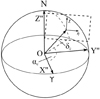 |
Fig. A.4 Relationship of the geocentric equatorial system with the coordinate system in picture plane. |
The position of the j particle in the picture plane is determined by unit vectors iN and iE, which are parallel to the directions to the north and east, respectively. The relationship of the geocentric equatorial system to the coordinate system in the picture plane is shown in Fig. A.4. The unit vectors iN and iE are determined from the equations
![Mathematical equation: \begin{equation*}\bm{i}_{\textrm{N}}=\left[\begin{array}{c}i^{x}_{\textrm{N}} \\i^{y}_{\textrm{N}} \\i^{z}_{\textrm{N}} \\\end{array}\right] =\left[\begin{array}{c}-\cos\alpha_{\textrm{c}}\sin\delta_{\textrm{c}} \\-\sin\alpha_{\textrm{c}}\sin\delta_{\textrm{c}} \\\cos\delta_{\textrm{c}} \\\end{array}\right],~\bm{i}_{\textrm{E}}=\left[\begin{array}{c}i^{x}_{\textrm{E}} \\i^{y}_{\textrm{E}} \\i^{z}_{\textrm{E}} \\\end{array}\right] =\left[\begin{array}{c}\sin\alpha_{\textrm{c}} \\\cos\alpha_{\textrm{c}} \\0 \\\end{array}\right].\end{equation*}](/articles/aa/full_html/2021/07/aa39668-20/aa39668-20-eq30.png) (A.11)
(A.11)
The coordinates χ and η of the j-particle in the picture plane are determined from the scalar product of unit vectors in the equatorial coordinate system:
![Mathematical equation: \begin{equation*}\left[\begin{array}{c}\chi_j(t) \\\eta_j(t) \\\end{array}\right] =\left[\begin{array}{c}\bm{\rho}_j(t)~\bm{i}_{\textrm{N}} \\\bm{\rho}_j(t)~\bm{i}_{\textrm{E}} \\\end{array}\right].\end{equation*}](/articles/aa/full_html/2021/07/aa39668-20/aa39668-20-eq31.png) (A.12)
(A.12)
In the proposed model, there is a restriction on the distance from the cometary nucleus, ρj ≤ 4 000 km. At larger distances, the acceleration of particles by SRP and the distribution of particle sizes should be taken into account.
References
- Afanasiev, V. L., & Moiseev, A. V. 2011, Balt. Astron., 20, 363 [NASA ADS] [Google Scholar]
- Afanasiev, V. L., & Amirkhanyan, V. R. 2012, Astrophys. Bull., 67, 438 [NASA ADS] [CrossRef] [Google Scholar]
- Afanasiev, V. L., Rosenbush, V. K., & Kiselev, N. N. 2014, Astrophys. Bull., 69, 211 [NASA ADS] [CrossRef] [Google Scholar]
- A’Hearn, M. F., Schleicher, D. G., Millis, R. L., et al. 1984, AJ, 89, 579 [NASA ADS] [CrossRef] [Google Scholar]
- Bagnulo, S., Tozzi, G. P., Boehnhardt, H., et al. 2010, A&A, 514, A99 [NASA ADS] [CrossRef] [EDP Sciences] [Google Scholar]
- Bagnulo, S., Belskaya, I., Cellino, A., et al. 2017, Eur. Phys. J. Plus, 132, 405 [CrossRef] [Google Scholar]
- Bauer, J. M., Grav, T., Blauvelt, E., et al. 2013, ApJ, 773, 22 [Google Scholar]
- Boehnhardt, H., Tozzi, G. P., Bagnulo, S., et al. 2008, A&A, 489, 1337 [NASA ADS] [CrossRef] [EDP Sciences] [Google Scholar]
- Bressi, T. H., McMillan, R. S., & Scotti, J. V. 2011, MPEC, 2011-L56 [Google Scholar]
- Bressi, T. H., Holmes, R., Vorobjov, T., et al. 2012, Central Bureau Electronic Telegrams, 3109 [Google Scholar]
- Brown, J. C., Potts, H. E., Porter, L. J., et al. 2011, A&A, 535, A71 [NASA ADS] [CrossRef] [EDP Sciences] [Google Scholar]
- Bus, S. J., A’Hearn, M. F., Schleicher, D. G., et al. 1991, Science, 251, 774 [NASA ADS] [CrossRef] [Google Scholar]
- Buzzi, L., Scotti, J. V., Gilmore, G., et al. 2012, MPEC, No. 2012-K12 [Google Scholar]
- Cochran, A. L., Cochran, W. D., & Barker, E. S. 1982, ApJ, 254, 816 [NASA ADS] [CrossRef] [Google Scholar]
- Djorgovski, S.,& Spinrad, H. 1985, ApJ, 90, 869 [CrossRef] [Google Scholar]
- Dones, L., Weissman, P. R., Levison, H. F., et al. 2004, Star Formation in the Interstellar Medium: In Honor of David Hollenbach, 323, 371 [Google Scholar]
- Dubovik, O., Sinyuk, A., Lapyonok, T., et al. 2006, J. Geophys. Res. (Atmos.), 111, D11208 [Google Scholar]
- Farnham, T. L., Schleicher, D. G., & A’Hearn, M. F. 2000, Icarus, 147, 180 [Google Scholar]
- Garcia, R. S., Gil-Hutton, R., & García-Migani, E. 2020, Planet. Space Sci., 180, 104779 [Google Scholar]
- Gunnarsson, M. 2003, A&A, 398, 353 [NASA ADS] [CrossRef] [EDP Sciences] [Google Scholar]
- Harris, A. W., & Harris, A. W. 1997, Icarus, 126, 450 [Google Scholar]
- Heiles, C. 2000, AJ, 119, 923 [NASA ADS] [CrossRef] [Google Scholar]
- Houpis, H. L. F., & Mendis, D. A. 1981a, Moon Planets, 25, 95 [Google Scholar]
- Houpis, H. L. F., & Mendis, D. A. 1981b, Moon Planets, 25, 397 [Google Scholar]
- Hsu, J.-C., & Breger, M. 1982, ApJ, 262, 732 [Google Scholar]
- Ivanova, A. V., Korsun, P. P., & Afanasiev, V. L. 2009, Solar Syst. Res., 43, 453 [Google Scholar]
- Ivanova, O. V., Luk’yanyk, I. V., Kiselev, N. N., et al. 2016, Planet. Space Sci., 121, 10 [Google Scholar]
- Ivanova, O., Rosenbush, V., Afanasiev, V., et al. 2017, Icarus, 284, 167 [Google Scholar]
- Ivanova, O. V., Picazzio, E., Luk’yanyk, I. V., et al. 2018, Planet. Space Sci., 157, 34 [Google Scholar]
- Ivanova, O., Luk’yanyk, I., Kolokolova, L., et al. 2019, A&A, 626, A26 [NASA ADS] [CrossRef] [EDP Sciences] [Google Scholar]
- Jewitt, D. 1991, IAU Colloq. 116: Comets in the post-Halley era, 19 [Google Scholar]
- Jewitt, D. 2015, AJ, 150, 201 [NASA ADS] [CrossRef] [Google Scholar]
- Jewitt, D., & Meech, K. J. 1986, ApJ, 310, 937 [Google Scholar]
- Jewitt, D. C., & Meech, K. J. 1987, ApJ, 317, 992 [Google Scholar]
- Kaňuchová, Z., Brunetto, R., Melita, M., et al. 2012, Icarus, 221, 12 [Google Scholar]
- Kartasheva, T. A., & Chunakova, N. M. 1978, Astrofizicheskie Issledovaniia Izvestiya Spetsial’noj Astrofizicheskoj Observatorii, 10, 44 [NASA ADS] [Google Scholar]
- Kimura, H., Kolokolova, L., & Mann, I. 2003, A&A, 407, L5 [NASA ADS] [CrossRef] [EDP Sciences] [Google Scholar]
- Kiselev, N., Rosenbush, V., Ivanova, O., et al. 2020, Icarus, 113768 [Google Scholar]
- Kolokolova, L., & Kimura, H. 2010, Earth Planets Space, 62, 17 [Google Scholar]
- Kolokolova, L., Das, H. S., Dubovik, O., et al. 2015, Planet. Space Sci., 116, 30 [Google Scholar]
- Korsun, P. P., Ivanova, O. V., & Afanasiev, V. L. 2006, A&A, 459, 977 [NASA ADS] [CrossRef] [EDP Sciences] [Google Scholar]
- Korsun, P. P., Ivanova, O. V., & Afanasiev, V. L. 2008, Icarus, 198, 465 [Google Scholar]
- Korsun, P. P., Rousselot, P., Kulyk, I. V., et al. 2014, Icarus, 232, 88 [Google Scholar]
- Korsun, P. P., Ivanova, O. V., Afanasiev, V. L., et al. 2016, Icarus, 266, 88 [Google Scholar]
- Kulyk, I., Rousselot, P., Korsun, P. P., et al. 2018, A&A, 611, A32 [NASA ADS] [CrossRef] [EDP Sciences] [Google Scholar]
- Lamy, P. L., Toth, I., Weaver, H. A., et al. 2011, MNRAS, 412, 1573 [Google Scholar]
- Larson, S. M. 1980, ApJ, 238, L47 [Google Scholar]
- Larson, S. M.,& Sekanina, Z. 1984, AJ, 89, 571 [Google Scholar]
- Maronna, R.A. & Yohai, V.J. 2017, Comput. Stat. Data Anal., 109, 64 [Google Scholar]
- Mazzotta Epifani, E., Dall’Ora, M., di Fabrizio, L., et al. 2010, A&A, 513, A33 [NASA ADS] [CrossRef] [EDP Sciences] [Google Scholar]
- Neckel, H., & Labs, D. 1984, Sol. Phys., 90, 205 [NASA ADS] [CrossRef] [Google Scholar]
- O’Dell, C. R., Robinson, R. R., Krishna Swamy, K. S., et al. 1988, ApJ, 334, 476 [Google Scholar]
- Oke, J. B. 1990, AJ, 99, 1621 [Google Scholar]
- Paganini, L., Mumma, M. J., Boehnhardt, H., et al. 2013, ApJ, 766, 100 [Google Scholar]
- Peixinho, N., Thirouin, A., Tegler, S. C., et al. 2020, The Trans-Neptunian Solar System, 307 [Google Scholar]
- Picazzio, E., Luk’yanyk, I. V., Ivanova, O. V., et al. 2019, Icarus, 319, 58 [NASA ADS] [CrossRef] [Google Scholar]
- Rauer, H., Arpigny, C., Boehnhardt, H., et al. 1997, Science, 275, 1909 [Google Scholar]
- Rauer, H., Helbert, J., Arpigny, C., et al. 2003, A&A, 397, 1109 [NASA ADS] [CrossRef] [EDP Sciences] [Google Scholar]
- Rosenbush, V. K., Ivanova, O. V., Kiselev, N. N., et al. 2017, MNRAS, 469, S475 [Google Scholar]
- Rosenbush, V., Ivanova, O., Kleshchonok, V., et al. 2020, Icarus, 348, 113767 [Google Scholar]
- Rousseeuw, P. J., & Bassett Jr, G. W. 1990, J. Am. Stat. Assoc., 85(409), 97 [Google Scholar]
- Samarasinha, N. H., & Larson, S. M. 2014, Icarus, 239, 168 [NASA ADS] [CrossRef] [Google Scholar]
- Sárneczky, K., Szabó, G. M., Csák, B., et al. 2016, AJ, 152, 220 [Google Scholar]
- Sekanina, Z. 1979, Icarus, 37, 420 [Google Scholar]
- Sekanina, Z., & Schuster, H. E. 1978, A&A, 68, 429 [Google Scholar]
- Schmidt, G. D., Elston, R., & Lupie, O. L. 1992, AJ, 104, 1563 [NASA ADS] [CrossRef] [Google Scholar]
- Storrs, A. D., Cochran, A. L., & Barker, E. S. 1992, Icarus, 98, 163 [Google Scholar]
- Vincent, J.-B., Böhnhardt, H., & Lara, L. M. 2010, A&A, 512, A60 [NASA ADS] [CrossRef] [EDP Sciences] [Google Scholar]
- Whipple, F. L., & Sekanina, Z. 1979, AJ, 84, 1894 [Google Scholar]
- Womack, M., Sarid, G., & Wierzchos, K. 2017, PASP, 129, 031001 [Google Scholar]
- Wong, I., & Brown, M. E. 2016, AJ, 152, 90 [Google Scholar]
The magnitudes graphs are available at http://www.aerith.net/comet/catalog/2011KP36/2011KP36.html
All Tables
Upper limits to the emission fluxes and production rates for undetected species CN, C2, and C3 in the spectrum of comet C/2011 KP36 (Spacewatch).
Best solutions for the coordinates of the north rotation pole of the nucleus of comet C/2011 KP36 (Spacewatch) and the cometocentric latitudes of the active areas.
Power index n in the dependence I ∝ 1∕ρn measured in the g-sdss and r-sdss images of comet C/2011 KP36 (Spacewatch).
Model parameters for different spatial brightness profiles in the g-sdss and r-sdss filters.
Characteristics of the dust coma of comet C/2011 KP36 (Spacewatch) determined by different methods.
Composition and size of the dust particles in different directions in the coma of comet C/2011 KP36 (Spacewatch) modeled with the rough spheroid model.
All Figures
|
Fig. 1 Long-slit spectrum of comet C/2011 KP36 (Specewatch) derived on November 25, 2016. (a) Energy distribution in the observed spectrum of the comet (black line) and the scaled Solar spectrum taken from Neckel & Labs (1984) (red line); (b) polynomial fitting of the cometary spectrum/Solar spectrum ratio; and (c) emission spectrum of the comet derived by subtracting the fitted continuum from the observed spectrum and the transmission curves of the g-sdss and r-sdss filters. |
| In the text | |
|
Fig. 2 Emissions of CO+ identified in the observed spectrum of comet C/2011 KP36 (Spacewatch). Calculated spectra of CO+ emissions are displayed at the bottom of the plot. |
| In the text | |
|
Fig. 3 Intensity maps of comet C/2011 KP36 (Spacewatch) in the g-sdss and r-sdss filters. (a) Direct images of the comet with the isophots differing by a factor |
| In the text | |
|
Fig. 4 Images of comet C/2011 KP36 (Spacewatch) in the r-sdss filter processed by a rotational gradient method. (a) Comparison of the observed (gray contours) and model jets: J1 is shown by red circles, J2 by blue circles, J3 and J4 by black circles. (b) Comparison of the observed and the modeled wave structure in the J4 jet (black). Directions to the Sun (⊙), north (N), east (E), and the negative velocity vector of the comet (V) are also provided. Negative distance is in the solar direction, and positive distance is in the antisolar direction. |
| In the text | |
|
Fig. 5 Schematic representation of the nucleus of comet C/2011 KP36 (Spacewatch) together with the rotational axis as viewed from the Earth and the model jets obtained during various phases of the nucleus rotation assumed for the moment of observations on November 25, 2016. The red spot is the active area located at the north hemisphere of the nucleus at the cometocentric latitude +75° (Source 1), and the active area at the south hemisphere at latitude −78° (Source 2) is depicted as a blue spot. The active area at the south hemisphere at latitude −5° (Source 3) is depicted as a black spot. The bright area is the area illuminated by the Sun at the moment of observation. A full period of the nucleus rotation is denoted by Pn and T denotes the rotational phase as a part of the rotation period. The arrows indicate the direction to the Sun (⊙), north (N), east (E), and anti-velocity vector of the comet in projection on the sky (–V). |
| In the text | |
|
Fig. 6 Observed surface brightness profiles of comet C/2011 KP36 (Spacewatch) in log–log representation for flux calibrated images acquired in g-sdss (a) and r-sdss (b) bands. The individual solid curves are cross-cuts measured from the photometric center of the comet through the coma along jets J1, J2, J3, and J4, while the cuts through the coma centered in the antisolar (PA = 56°) and solar (PA = 236°) directions are marked as the dashed lines. The innermost data points that may be affected by seeing, bounded by a vertical dotted line, were not considered. Short black lines represent the canonical profile, in which the brightness varies with cometocentric distance ρ as I ∝ 1∕ρ. |
| In the text | |
|
Fig. 7 Normalized surface brightness profiles of comet C/2011 KP36 (Spacewatch) and a field star (dotted line) measured in the g-sdss and r-sdss images. Profiles are taken across the central region of the comet along jets J1 and J2 located in the solar and antisolar directions (solid line) and jets J3 and J4 located close to perpendicular to the solar-antisolar direction (dashed line). |
| In the text | |
|
Fig. 8 Modeled and observed brightness profiles in comet C/2011 KP36 (Spacewatch) in the g-sdss and r-sdss filters along the directions with the position angles of 8° (jet J4, plot a), 56° (coma C1, plot b), 146° (coma C2, plot c), and 261° (jet J1, plot d). The observed and modeled profiles are designated by a black solid line and a dotted line, respectively. The coma profile is shown by a dashed line, and the calculated profile for the comet nucleus by a gray solid line. Negative distance is in the solar direction, and positive distance is in the antisolar direction. |
| In the text | |
|
Fig. 9 g – r color map (left panel) and polarization map in the r-sdss filter (right panel) of comet C/2011 KP36 (Spacewatch) observed on November 25, 2016 at the phase angle 9.6°. Corresponding scale bars in magnitude for the color map and in percentage for the polarization map are displayed at the top of the images. The location of the optocenter is marked by a black cross, jets by black lines, and the possible shell and arcs are indicated by white dotted lines. The arrows point in the direction to the Sun (⊙), north (N), east (E), and the negative velocity vector of the comet as seen in the observer’s plane of sky (V). Negative distance is in the solar direction, and positive distance is in the antisolar direction. |
| In the text | |
|
Fig. 10 Distribution of the polarization vectors in the coma of comet C/2011 KP36 (Spacewatch). The orientation of the vectors indicates the direction of the local polarization plane, and the length of the vectors marks the degree of polarization. The arrows point in the direction to the Sun (⊙), north (N), east (E), and the negative velocity vector of the comet as seen in the sky plane (V). Negative distance is in the solar direction, and positive distance is in the antisolar direction. |
| In the text | |
|
Fig. 11 Radial profiles across the g – r color (top panel) and polarization (bottom panel) maps of comet C/2011 KP36 (Spacewatch). The individual curves are scans measured from the photometric center of the comet through the J1, J2, J3, and J4 jets and the coma in different directions: the solid black line is the cuts along the J1and J2; the dotted line is the cuts along the J3 and J4; the solid gray line is the cuts across the nucleus and coma in the directions with PA = 56° and PA = 236°. The radial profiles of the dust color without the nucleus contribution are marked by colored lines. Zero point is at the photometric center of the comet. Vertical dashed lines show the size of the seeing disc during the observations. Negative distance is in the solar direction, and positive distance is in the antisolar direction. |
| In the text | |
|
Fig. 12 (a) Single-sided amplitude spectrum of the spatial frequencies of color profiles for jets J1 and J2 in comet C/2011 KP36 (Spacewatch) observed on November 25, 2016. (b) Comparison of the spatial color profiles forthe J3 and J4 jets with different distance scales from the nucleus of the comet to demonstrate the correlation between the profiles. The dashed line shows the magnitude of the random signal at 2.5σ level. |
| In the text | |
|
Fig. A.1 Coordinate system {XYZ} on the nucleus surface. |
| In the text | |
|
Fig. A.2 Coordinate system {X′ Y′ Z′} associated with the precession of the nucleus. |
| In the text | |
|
Fig. A.3 Transition from the coordinate system {X′ Y′ Z′} associated with the precession of the rotational axis of the nucleus to the equatorial cometocentric coordinate system {X′′ Y′′ Z′′}. |
| In the text | |
|
Fig. A.4 Relationship of the geocentric equatorial system with the coordinate system in picture plane. |
| In the text | |
Current usage metrics show cumulative count of Article Views (full-text article views including HTML views, PDF and ePub downloads, according to the available data) and Abstracts Views on Vision4Press platform.
Data correspond to usage on the plateform after 2015. The current usage metrics is available 48-96 hours after online publication and is updated daily on week days.
Initial download of the metrics may take a while.