| Issue |
A&A
Volume 650, June 2021
|
|
|---|---|---|
| Article Number | A33 | |
| Number of page(s) | 12 | |
| Section | Extragalactic astronomy | |
| DOI | https://doi.org/10.1051/0004-6361/202140597 | |
| Published online | 03 June 2021 | |
A systematic search for changing-look quasars in SDSS-II using difference spectra
Department of Physics, University of Bath, Claverton Down, Bath BA2 7AY, UK
e-mail: This email address is being protected from spambots. You need JavaScript enabled to view it.
Received:
17
February
2021
Accepted:
16
April
2021
Abstract
Context. ‘Changing-look quasars’ (CLQs) are active galactic nuclei (AGN) showing extreme variability that results in a transition from type 1 to type 2 AGN. The short timescales of these transitions present a challenge to the unified model of AGN and the physical processes causing these transitions remain poorly understood. CLQs also provide interesting samples for the study of AGN host galaxies since the central emission disappears almost entirely.
Aims. Previous searches for CLQs have utilised photometric variability or SDSS classification changes to systematically identify CLQs; this approach may miss lower luminosity CLQs. In this paper, we aim to use spectroscopic data to asses if analysis difference spectra can be used to detect further CLQs that have been missed by photometric searches.
Methods. We searched SDSS-II DR 7 repeat spectra for sources that exhibit either a disappearance or appearance of both broad line emission and accretion disc continuum emission by directly analysing the difference spectrum between two epochs of observation.
Results. From a sample of 24 782 objects with difference spectra, our search yielded six CLQs within the redshift range 0.1 ⩽ z ≤ 0.3, including four newly identified sources. Spectral analysis indicates that changes in the accretion rate can explain the changing-look behaviour. While a change in dust extinction fits the changes in the spectral shape, the timescales of the changes observed are too short for obscuration from torus clouds.
Conclusions. Using difference spectra was shown to be an effective and sensitive way to detect CLQs. We recover CLQs an order of magnitude lower in luminosities than those found by photometric searches and achieve higher completeness than spectroscopic searches relying on pipeline classification.
Key words: galaxies: active / accretion / accretion disks
© ESO 2021
1. Introduction
Active galactic nuclei (AGN) are known to be variable on timescales of months to years (e.g. MacLeod et al. 2010). Their variability is generally associated with instabilities in the accretion disc. AGN are also found in two general types, type 1 and 2, the first of which shows strong broad emission lines and continuum emission, while the latter shows neither. These two types are generally explained as being due to orientation effects (Antonucci 1993; Urry & Padovani 1995). Only a small subset of AGN show continuum variability strong enough so that accretion disc emission appears or disappears entirely, accompanied with an appearance or disappearance of broad line emission. These objects are commonly referred to as ‘changing-look quasars’ (CLQs). In this paper, we define changing-look behaviour to be a clear transition between AGN types, irrespective of luminosity.
Changing-look quasars are relatively rare, but a notable well-researched example from the last 40 years is NGC 4151 (e.g. Osterbrock 1977; Antonucci & Cohen 1983; Penston & Perez 1984; Lyutyi et al. 1984; Shapovalova et al. 2010), which has been observed ‘flickering’, as it transitioned back and forth between classification types. The first CLQ with quasar luminosity1, SDSS J015957.64+003310.5 (hereafter referred to as J0159+0033), was identified by LaMassa et al. (2015). Subsequently, a number of similar objects have been identified (e.g. Runnoe et al. 2016; Ruan et al. 2016; MacLeod et al. 2016, 2019; Gezari et al. 2017; Yang et al. 2018; Ross et al. 2018; Stern et al. 2018).
There are a number of proposed scenarios that could explain changing-look behaviour. A popular explanation is that the observational variability is caused by a significant change in the accretion rate onto the central black hole. This drop in ionising flux causes a dimming of the broad line emission, while the narrow line region (NLR) remains unchanged due to the longer light travel time. Such a sudden change in ionising flux could be caused by instabilities in the disc or accretion state transitions (Noda & Done 2018). Such a change could either be gradual, with AGN transitioning from high to low accretion states, or stochastic, with objects experiencing repeated extreme changes in accretion (e.g. Penston & Perez 1984; Elitzur et al. 2014). Alternatively, the movement of an isolated dust cloud in the torus can cause a change in extinction along the line of sight that would produce extreme broad line variability (Nenkova et al. 2008). This mechanism is disfavoured for some cases (e.g. J0159+0033, LaMassa et al. 2015) based on the timescale of the transition, but it could be responsible for some changing-look behaviour. Another alternative explanation for changing-look behaviour are tidal disruption events (TDEs; e.g., Eracleous et al. 1995; Merloni et al. 2015). Merloni et al. (2015) propose that a luminous flare caused by the tidal disruption of a star near a supermassive black hole (SMBH) could have led to the observations of changing-look behaviour in J0159+0033. TDEs, however, cannot explain NLR emission on large scales ionised by the AGN. Studying changing-look behaviour can therefore give insights into accretion disc physics (Noda & Done 2018), the structure of the obscuring torus (Nenkova et al. 2008), as well as the incidence of TDEs.
To date there have been four systematic searches for CLQs, yielding a total of 50 CLQs (Ruan et al. 2016; MacLeod et al. 2016, 2019; Yang et al. 2018). These data sets provide an invaluable resource for analysing the likely physical mechanisms causing changing-look behaviour. Previous systematic CLQ searches have used either changes in the classification of objects in survey pipelines or on large photometric changes to identify objects of interest.
This focus on spectral classification changes and photometric variability favours the most obvious CLQs. In this work, we aim to assess the novel method of using difference spectra to identify CLQs, and to detect additional CLQs missed by previous searches of repeat spectra from SDSS-II. We directly measure broad emission and continuum variability shown in the difference between two epochs, and use them as sample selection criteria.
The outline of this paper is as follows. Section 2 presents the method of using difference spectra to identify CLQ. Section 3 presents the results of the search, describing a sample of six CLQs, including four newly identified sources, the spectral decomposition method used to separate the host galaxy and the quasar components, and the emission line fitting procedure used to measure the broad emission lines and estimate the mass of the central SMBH. Section 4 investigates variable accretion rate and variable obscuration as explanations for the six CLQs. Section 5 summarises and makes concluding comments. Where needed, we adopt a flat Λ cold dark matter cosmology, where H0 = 69.6 km s−1 Mpc−1 and ΩM = 0.286.
2. SDSS spectroscopic data search
Our search for CLQs directly compared repeat spectroscopy from SDSS DR7 by constructing a ‘difference spectrum’ for each object in our sample to identify changing-look behaviour. By analysing the difference spectrum in our search methodology, we hoped to isolate and measure the variable component between epochs of observation. We aimed to show that our search is sensitive to changing-look behaviour by identifying new CLQs from SDSS-II.
2.1. Spectroscopic data
We used the spectroscopic data from the final SDSS-I/II data release 7 (DR7). DR7 contains 1 630 960 spectra, including 929 555 galaxy spectra and 121 363 quasar spectra (Abazajian et al. 2009). SDSS-I/II spectra are captured using a 3″ diameter fibre and have a wavelength coverage of 3800 to 9200 Åat a resolution of R ≈ 2000 (York et al. 2000). We used the classification made by the SDSS spectroscopic pipeline (see Stoughton et al. 2002) to select objects classified as either a galaxy (GALAXY) or a quasar (QSO). We did not rely on changes in classification between repeat spectra. We included all objects with at least two different epochs of observation.
We chose SDSS DR7 to ensure all spectra were captured with only the SDSS Legacy spectrograph. This removes any potential false positive detections due to instrumental changes. Since the aim of this work was to show how spectroscopic searches can be used to expand on photometric searches, rather than create large samples of CLQs, SDSS DR7 data alone is used. All observed spectra shown were corrected for galactic extinction using the extinction law of Fitzpatrick (1999), and the maps of Schlegel et al. (1998).
2.2. Sample selection
A super-set of candidate CLQs was selected using the following criteria. Firstly, each object must have repeat spectra in SDSS DR7 in at least two different epochs. Secondly, each object must be classified as either GALAXY or QSO in all epochs of observation, rejecting stars. Finally, each object must have redshift, 0.1 ≤ z ≤ 0.4 to ensure that both Hα and the blue continuum at ∼3500 Å are visible. The resulting super-set consisted of 55 116 spectra from 24 782 objects.
Changing-look behaviour is defined as a clear transition between AGN types. An AGN exhibiting a convincing type transition in the optical possesses at least two features: a strongly brightening or dimming continuum and broad line variability across its multi-epoch spectra. We identified CLQs by quantifying these two changing-look features using the difference spectrum, |Δfλ| = |fepoch2−fepoch1|. The observed spectra were smoothed using a Gaussian filter before computing the difference spectrum to reduce the effect of noise. We modelled the continuum as a third-degree polynomial and fitted to the entire wavelength range available on the difference spectrum. This fit was used to subtract the continuum and isolate emission lines.
As an initial step, we preselected objects showing considerable continuum variability at 4100–5500 Å (corresponding to the SDSS g-band). We selected objects with a variability exceeding 3 × 10⁻¹⁸ erg s−1 cm−2 Å−1 corresponding to Δmag ∼ 0.16 at a magnitude of 21. If variability is caused by changes in the accretion rate, we expect the difference spectrum continuum of a CLQ to resemble a Shakura-Sunyaev accretion disc power law (Shakura & Sunyaev 1973).
In a variable obscuration scenario, blue light would be attenuated more than red (Vanden Berk et al. 2004; Wilhite et al. 2005; Schmidt et al. 2012). Similarly, in a variable accretion rate scenario stronger changes are expected at short wavelength due to the spectrum of the accretion disc. Consequently, we searched difference spectra for a strong blue continuum.
We used the mean slope of the polynomial-continuum in the wavelength range 3500 to 3700 Å to characterise the strength of the continuum variability. Three threshold values, listed in Table 1, quantitatively define weak, intermediate, and strong detections of continuum variability.
Changing-look identifier thresholds.
Changing-look broad line variability is measurable as it manifests itself in the difference spectrum as apparent broad emission lines. We specifically searched for the strongest optical broad emission lines: Hβ; and Hα, by extracting our modelled continuum from the difference spectrum, and then identifying the highest monochromatic flux in the rest wavelength ranges 4856–4866 Å and 6558–6568 Å, respectively. For a CLQ, we expect only broad lines to appear in the difference spectrum since narrow lines are not expected to vary over short timescales due to extra light travel time from the continuum source to the narrow line region, relative to the broad line region (BLR). So, at this stage we were not concerned with measuring the width of the emission in the above wavelength range, only the flux. Three threshold values each for the detected Hα and Hβ emission line flux, listed in Table 1, were used to define weak-, intermediate-, and strong-cases of broad emission line variability2. Objects that displayed both changing-look indicators (except those with only weak detections of both continuum and broad line variability), or a strong-case of one changing-look indicator, were selected as changing-look candidates.
In summary, our selection algorithm first separated the continuum for emission lines, then accepted objects with continuum variability in the range 4100–5500 Å greater than Δmag ∼ 0.16 at a magnitude of 21. We then quantified the changing-look indicators, blue continuum variability and broad emission line variability, and applied thresholds listed in Table 1 to complete our search.
The search yielded 941 CLQ candidates. We visually inspected all candidate spectra, rejecting quasars that show variability, but do not exhibit an AGN type transition. We identified a total of six CLQs, four of which are newly identified and evidence the sensitivity of the systematic difference spectrum search methodology. Two CLQs, J135855.83+493414.2 (hereafter referred to as J1358+4934), found by Yang et al. (2018), and J012648.08-083948.0 (hereafter referred to as J0126-0839), found by Ruan et al. (2016), were recovered. Yang et al. (2018) finds two other CLQs from SDSS Legacy repeat spectra (see Table 5 of Yang et al. 2018), and these were also recovered by the sample selection algorithm, yet excluded from the analysis in the interest of only including those objects displaying the clearest and strongest changing-look behaviour. Sample selection cuts that were made are shown in Table 2.
CLQ sample selection cuts.
To assess the validity of the sample selection methodology, we also applied the sample selection algorithm to the SDSS Legacy and BOSS spectra of the MacLeod et al. (2016) CLQs. Our sample selection algorithm recovered seven of the ten objects identified by MacLeod et al. (2016). The three missing objects were not recovered using our method as they were either outside our redshift range criterion or missing data in the relevant spectral range.
3. The changing-look quasars
Our difference spectrum search method identified six CLQs in SDSS-II, including four newly found sources using the difference spectrum method developed here. Two CLQs ‘turned off’ (disappearing broad lines and continuum), three ‘turned on’ (appearing broad lines and continuum), and one was observed to ‘turn off and turn on’ (disappearing and reappearing broad lines and continuum, after an additional BOSS spectrum was identified). The properties of the final sample of CLQs are listed in Table 3. The objects have redshifts 0.116 ≤ z ≤ 0.295.
CLQs found.
3.1. Turning off CLQs
The two CLQs that turned off are displayed in Fig. 1. In the first epoch of observation of both objects, the AGN classification is type 1, and the Hβ broad line completely disappears by the second epoch of observation.
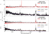 |
Fig. 1. Observed spectra and the difference spectrum of the turning off CLQs. The quasars shown are J0823+4220 (top two panels), and J0126–0839 (bottom two panels). Upper: the observed optical spectra, with the first epoch (black) and second epoch (red) both shown. Lower: the difference spectrum |Δfλ| (black) is shown, demonstrating how the CLQs were identified, and the resemblance of the variable component to an accretion disc. A fitted Shakura-Sunyaev accretion disc power law fυ ∝ υ1/3 (dashed-blue) and a best-fit power law to the continuum (orange) is shown. |
The object J082323.89+422048.3 (hereafter referred to as J0823+4220) is shown in the top panel of Fig. 1. In its second epoch of observation, a relatively strong Hα broad line remains, which characterises its AGN type as type 1.9. The transition happened on a timescale of 2258 days (1950 days in the rest frame).
The object J0126–0839, which was first found by Ruan et al. (2016), is shown in the bottom panel. J0126–0839 has the most extreme changing-look behaviour observed in the sample as both Hβ and Hα completely disappear. A disappearing Hγ broad line is also evident, particularly in the difference spectrum (black curve). The AGN has transitioned to type 2 in its second epoch of observation on a time scale of 2302 days (1902 days in the rest frame).
3.2. Turning on CLQs
The three CLQs that turned on are displayed in Fig. 2. In the second epoch of observation of all three objects, the AGN classification is type 1, as strong Hβ and Hα broad emission lines have emerged. We note that all three display asymmetry in their bright-state broad emission of both Hβ and Hα, the broad emission lines show excess emission in the red wing. Similar asymmetry is not exhibited in the CLQs that turned off.
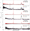 |
Fig. 2. Observed spectra and the difference spectrum of the turning on CLQs. The turning on CLQs are shown in the same format as Fig. 1. The quasars shown are J1723+5504 (top two panels), J0829+4154 (middle two panels), and J1358+4934 (bottom two panels). |
The object J172322.31+550413.8 (hereafter referred to as J1723+5504), shown in the top panel of Fig. 2, transitioned from a type 1.83 to type 1 AGN in just 184 days (142 days in the rest frame). To our knowledge, this is the fastest observed changing-look behaviour in a distant AGN with quasar luminosity. In its first epoch the presence of a weak broad Hβ characterises J1723+5504 as an intermediate type 1.8. The Hβ and Hα broad lines clearly emerge by the second epoch. The broad Hβ and Hα are asymmetric in the bright-state epoch, with an extended red wing.
The object J082942.67+415436.9 (hereafter referred to as J0829+4154) is shown in the middle panel. Similar to J1723+5504, it is in an intermediate state in its first epoch: type 1.8. The observed broad components of Hα and Hβ appear to be either asymmetric with a red wing, as with that of J1723+5504, or are substantially redshifted with respect to their narrow components, in both the dim- and bright-state. The transition happened on a timescale of 2258 days (2005 days in the rest frame).
The object J1358+4934, which was first identified by Yang et al. (2018), is shown in the bottom panel. J1358+4934 shows the most extreme turning on changing-look behaviour in the sample as it transitions from AGN type 2 to type 1. To a less obvious extent than J1723+5504 and J0829+4154, J1358+4934 is also asymmetric in the emerging Hα and Hβ emission with a red wing in its bright-state spectrum. The transition happened on a timescale of 1115 days (999 days in the rest frame).
3.3. Turning off and on changing-look quasar
The multi-epoch spectra and difference spectra of J000236.25-002724.8 (hereafter referred to as J0002-0027) are shown in Fig. 3. The object was observed twice in SDSS-II, shown by the black and red curves in the top panel of Fig. 3, and was identified from these spectra. The continuum dimmed, the Hβ broad line disappeared, and the Hα broad line diminished, yet remained strong relative to Hβ, as the object turned off in transitioning from type 1 to type 1.9. The object exhibited this changing-look behaviour in 768 days (587 days in the rest frame). J0002-0027 was re-observed by SDSS-III BOSS, giving us an additional third epoch of observation (blue curve). The re-appearing broad emission lines and continuum from the third epoch almost perfectly match that of the first epoch. The only major observational difference to the first epoch spectrum is a blue excess in the broad Hα emission in the BOSS spectrum. No such excess is seen in Hβ and the width and shape of the line is otherwise unchanged, as shown by the bottom-right panel of Fig. 3. Overall, the object was observed turning off and on in 3686 days total (2818 days in the rest frame).
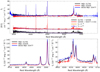 |
Fig. 3. Observed spectra and the difference spectra of the turning off and on CLQ J0002-0027. Top: the three observed spectra, including the extra BOSS spectrum (blue curve), are shown in the SDSS Legacy rest wavelength range of the object. The epochs for the black, red, and blue spectra are MJD = 51791, 52559, and 55477, respectively. Middle: the difference spectra of the first and second epoch (black curve), and the second and third epoch (red) are shown on the same flux scale, with a constant added to the latter. Bottom: a zoomed in view of the observed spectra in the Hβ (left) and Hα (right) regions is shown. |
3.4. Spectral analysis
In the following section, we describe the spectral analysis performed to characterise the shape of the variable component, fit narrow and broad emission lines and measure black hole masses and Eddington ratios.
3.4.1. Continuum variability
The difference spectrum (black curve in alternating panels of Figs. 1 and 2, black and red curves in the middle panel of Fig. 3) shows the variable component, exhibiting a blue continuum. We fitted the spectrum with a power-law |Δfλ| ∝ λ−β (orange curve) as well as a standard thin accretion disc power-law of form fυ ∝ υ1/3 (dashed blue curve) (Shakura & Sunyaev 1973). For the fit, we masked regions around prominent Balmer emission lines (Hα: 6420 to 6800 Å; Hβ: 4770 to 5050 Å; Hγ: 4280 to 4400 Å; and Hδ: 4050 to 4140 Åfor J0126-0839). The difference spectrum of all six CLQs was well fitted by a standard thin disc model. The variability is therefore consistent with changes in the accretion rate.
3.4.2. Spectral decomposition
We intended to derive the black hole mass and characterise the source of ionisation in the narrow line region. In order to isolate the AGN continuum, and the broad and narrow emission lines, we decomposed the observed spectra of the CLQ sample into host-galaxy and quasar components. Additionally, we used the decomposed spectra to determine if variable obscuration of the disc component can explain the observed behaviour.
To decompose the spectra, we used a modified version of the method by Vanden Berk et al. (2006), who fitted spectra with quasar and galaxy eigenspectra. Specifically, we used the first five SDSS galaxy and the first five SDSS quasar eigenspectra described and made available by Yip et al. (2004a) and Yip et al. (2004b), respectively. We fitted linear combinations of the eigenspectra, with their coefficients as ten free parameters, to the observed spectra using a χ2 minimisation. Yip et al. (2004a,b) showed that their galaxy and quasar eigenspectra gave a statistical coverage of 98.37% and 99.81% of their respective SDSS samples used to generate them. We masked the Hβ and Hα regions (4780 to 5080 Åand 6270 to 6800 Å) due to the complexity of the broad emission lines. Aside from broad line masking, the decomposition was performed for the maximum available rest wavelength range of each object. All SDSS-II spectra are observed using a 3″ diameter fibre, and we did not expect any intrinsic variability in the host galaxy over the relatively short timescales of our sample, meaning the observed host component should remain constant across repeat spectra. Hence, we decomposed repeat SDSS-II spectra of each object simultaneously while constraining the galaxy eigenspectrum coefficients as equal across all epochs of observation.
The result of decomposition for each spectrum were isolated galaxy (blue curve) and quasar (green) components, shown in Fig. 4 for J0823+4220 with their sum (red) as an example result. Similarly to Fig. 4, the other spectra were fitted well by our model. J0126-0839, which transitioned from a type 1 to type 2 AGN (the most extreme changing-look behaviour in the sample), was best fitted with zero quasar component in its second epoch spectrum.
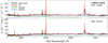 |
Fig. 4. Spectral decomposition of the CLQ J0823+4220, which turned off. The fitted galaxy (blue curve) and quasar (green) components, and their sum (red) from the best-fit eigenspectrum coefficients (found as per Sect. 3.4.2) are shown. Top: the earlier epoch (MJD = 52266) bright-state spectrum. Bottom: the later epoch (MJD = 54524) dim-state spectrum. |
3.4.3. Broad and narrow emission line fitting
To measure the broad and narrow emission lines of only the quasar component of each spectrum, we used the host-galaxy component (blue curve in Fig. 4) yielded by the spectral decomposition of Sect. 3.4.2 and subtracted it directly from each observed spectrum (black curve in Fig. 4). We chose to subtract the host galaxy from the observed to preserve as much detail from the observed spectrum as possible, rather than simply using the quasar component from Sect. 3.4.2. Narrow emission is present in the host-galaxy component. Since we aimed to analyse the observed narrow line emission, we did not subtract any narrow emission from the observed. We masked the narrow lines in the host galaxy component before subtracting it (Hβ, [OIII] 4959 Å, [OIII] 5007 Å, Hα, [NII] 6548 Å, [NII] 6583 Å, [SII] 6716 Å, and [SII] 6731 Å). We refer to the resulting spectrum hereafter as the ‘decomposed AGN spectrum’.
We fitted the full wavelength range of each decomposed AGN spectrum with a power law continuum, and a collection of broad and narrow Gaussians. A single Gaussian was fitted to the following narrow emission lines: the [OIII] doublet; the [NII] doublet; and the [SII] doublet. The Hβ and Hα were fitted with two Gaussians representing both a broad and narrow component. We distinguished between broad and narrow emission lines by constraining their Gaussian line widths. We constrained the broad lines to have velocity width > 1200 km s−1, and narrow lines < 1200 km s−1 (Hao et al. 2005).
It is also known that the NLR is stratified based on ionisation, with the high ionisation lines arising from the inner NLR, and the low ionisation lines arising from the outer NLR (e.g. Veilleux 1991). As a result, we constrained the velocity and width of the narrow lines in ionisation groups. Hβ and Hα are one group; the [NII] doublet and the [SII] doublet are another; and the [OIII] doublet forms the last group. Narrow lines within groups were constrained to have identical width and velocities. The width and velocities of the broad Hβ and Hα were left as free parameters.
Because of extra light travel time from the continuum source to the NLR relative to the BLR, we did not expect any intrinsic variability in the narrow emission. Hence, the repeat decomposed AGN spectra of each object were fitted simultaneously4, while constraining the narrow lines to be equal across repeat spectra. Broad emission and the power law AGN continuum were left free to vary across repeat spectra5.
The measured broad Hβ and Hα properties are listed in Table 4. The best fit to the decomposed AGN spectrum (dashed red curve) of J0823+4220 is shown in Fig. 5 as an example. The spectra, including emission lines, were well fitted for the entire sample with two minor discrepancies.
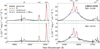 |
Fig. 5. Emission line fitting to the decomposed AGN spectrum (black) of the CLQ J0823+4220. The AGN spectrum was fitted (red) with a power law continuum (green) and a selection of narrow and broad Gaussians. The fitting procedure is described in Sect. 3.4.3. |
Measured and inferred CLQ properties.
Number of CLQs that were observed turning-off, turning-on, and both.
Firstly, the power law continuum fails to represent the full level of detail in the wavelength range 3400 to 4500 Å. Secondly, due to the use of a single Gaussian for the broad lines, asymmetries observed in the broad lines of the ‘on-state’ spectra are not fully fitted in the wings of the line (e.g. bright-state Hβ and Hα broad lines of J1723+5504, both spectra of J0829+4154, and in the bright-state Hα broad line of J1358+4934). However, for our purpose of measuring the broad and narrow line velocity dispersion and fluxes, the fits are acceptable.
3.5. Black hole mass and Eddington ratios
From measurements of the decomposed AGN spectrum continuum and emission lines made in Sect. 3.4.3, we can estimate the black hole mass MBH and the Eddington ratio λedd = Lbol/LEdd of the six CLQs. We used Hα for the black hole mass measurement because four of the six CLQs retain a relatively strong broad Hα compared to the Hβ in their dim-state spectra. Therefore, the Hα-derived black hole mass was better for use as a comparative measure across the repeat spectra. We used the black hole mass the equation from Greene et al. (2010):
![Mathematical equation: $$ \begin{aligned} {M}_{\mathrm{BH}}&= 9.7 \times 10^6 \left[ \frac{{FWHM}(\mathrm{H} \alpha )}{1000\,\mathrm{km}\,\mathrm{s}^{-1}} \right] ^{2.06} \nonumber \\&\quad \times \left[ \frac{\lambda L_{5100}}{10^{44} \, \mathrm{erg}\,\mathrm{s}^{-1}} \right] ^{0.519} \, {M}_{\odot } , \end{aligned} $$](/articles/aa/full_html/2021/06/aa40597-21/aa40597-21-eq1.gif) (1)
(1)
using the FWHM of the Hα broad emission and the monochromatic rest 5100 ÅAGN luminosity λL5100 from the fitted power law continuum.
The bolometric luminosity Lbol of the CLQs was estimated by applying the linear bolometric correction of 8.1 from Runnoe et al. (2012) to the measured λL5100. The Eddington ratio was then Lbol/LEdd where LEdd was found from the Hα-estimated BH mass from Eq. (1), as LEdd = 1.25 × 1038MBH/M⊙. All inferred AGN properties are listed for each repeat observation in the sample in Table 4.
The CLQs have black hole masses in the range 7 × 10⁷ to 7.2 × 10⁸ M⊙. Black hole masses derived for each object across the repeat spectra are within 0.2 dex generally consistent within the uncertainties. The CLQs have Eddington ratios in the range 0.006 to 0.04. This shows that all six CLQs are hosted by massive black holes, with accretion rates well below the Eddington limit.
3.6. Narrow emission line analysis
The size of the NLR means that light travel time from the continuum source to the NLR is ∼103 − 4 years, compared to ∼101 − 2 days to the BLR (e.g. Antonucci 1993; Urry & Padovani 1995). Narrow line emission can therefore constrain the photoionisation mechanism of the NLR gas over the last 103 − 4 years. The observed [OIII]/Hβ and [NII]/Hα line ratios, measured as described in Sect. 3.4.3, of all the CLQs are shown in Fig. 6 on a BPT diagram (Baldwin & Phillips 1981). We include the BPT classification schemes of Kauffmann et al. (2003) and Kewley et al. (2006) to distinguish between objects whose emission is dominated by either AGN or star formation. The AGNs are further categorised into Seyfert AGNs and low ionisation nuclear emission line regions (LINERs) by the scheme of Schawinski et al. (2007).
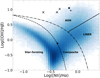 |
Fig. 6. BPT diagram showing the narrow emission line ratios of the six CLQs, three turning on (cross) and two turning off (star), and one turning off then on (plus). The heat map was produced using the MPA-JHU emission line analysis of 927 552 DR7 objects, thereby showing the overall SDSS trend (Brinchmann et al. 2004). Three emission line classification schemes are shown. Kauffmann et al. (2003) (dashed line) separates star-forming and composite host galaxies, Kewley et al. (2006) (dotted line) separates AGN and composite host galaxies, and Schawinski et al. (2007) separates LINERs from AGN. |
Figure 6 shows that all of the CLQs’ emission lines were ionised either fully or partially by an AGN continuum, including J0126-0839, which is classified in the composite region. Its emission line ratios are likely caused by strong star formation in its host galaxy. Kauffmann et al. (2003) estimate that an AGN continuum contributes between 30 and 90 per cent of the ionising emission for objects in this region. NLR ionisation by an AGN disfavours the TDE scenario proposed by Merloni et al. (2015). They propose that the changing-look behaviour exhibited by the object identified by LaMassa et al. (2015) (J0159+0033) was produced by observation of the object during and after a luminous flare caused by the tidal disruption of a star passing by a SMBH. For such an observation, we expect narrow line ratios more indicative of star-formation. Following Ruan et al. (2016), we also examined the flux of the strongest narrow line, [OIII] 5007 Å, to further test the plausibility of the TDE scenario. Measured [OIII] 5007 Å line fluxes of the sample yielded luminosities in the range 0.8–25 × 1041 erg s−1. This is in contrast with fluxes measured in typical TDEs, which have significantly fainter [OIII] 5007 Å emission. It is unlikely, then, that the observed variability in these CLQs was caused by a TDE (e.g. Gezari et al. 2006, 2009, 2012).
The NLR in all three turning on CLQs have been ionised by an AGN-like continuum source. If we assume that in the ‘off-state’ the AGN continuum emission has dimmed significantly, this implies that all three objects have not remained in the off-state for the last ∼103 − 4 years, but instead have been in a state of flickering. The flickering could be an important part of AGN evolution. If we assume an equal likelihood of observing a flickering CLQ in the on or off state, that idea is encouraged by the identification of an equal number of turning off and turning on CLQs.
4. Discussion
We have used difference spectra to search for CLQs in SDSS DR7 without pre-selecting on photometric variability or a change in spectral classification in the pipeline. We identified six CLQs, four of which are newly discovered using the difference spectrum method developed here. This shows that the approach presented can be very effective for finding CLQs and could be extended to higher redshift by using different broad lines or different spectroscopic datasets, including SDSS-BOSS spectra.
4.1. Comparison to other CLQ searches
There have been three systematic searches that yielded a total of 50 CLQs to date (Ruan et al. 2016; MacLeod et al. 2016, 2019; Yang et al. 2018). Previous searches relied on changes in object classification or large photometric variability to select CLQs. Here, we compare the properties of the previously selected CLQs to those selected here using difference spectra.
Ruan et al. (2016) first identified the CLQ J0126-0839, which is also recovered in this paper, from the object’s SDSS-II spectra. They showed that the object, whose classification transitioned from galaxy-like to quasar-like, is very likely to display changing-look behaviour. Ruan et al. (2016) included BOSS spectra (SDSS DR12) in their search, which yielded one additional new CLQ, J233602.98+001728.7 (hereafter referred to as J2336+0017), and the recovery of J0159+0033, which was first identified by LaMassa et al. (2015). The identified CLQs have luminosities 42.30 ⩽ log10(λL5100) ⩽43.56 with a median of 43.43, comparable to the luminosities in our sample.
MacLeod et al. (2016) propose that significant broad emission line (BEL) variability will be associated with at least a 1.0 mag variability of the g-band photometry of a CLQ. They used repeat photometry from SDSS and Pan-STARRS1 to select CLQ candidates, and confirmed nine new CLQs, spanning the redshift range 0.204 ⩽ z ⩽ 0.625, using repeat spectroscopy in both SDSS-II and BOSS (SDSS-III). MacLeod et al. (2019) extended this work by expanding their photometric search to include highly variable objects in SDSS-II that did not possess any BOSS spectra. They confirmed 17 new CLQs using optical spectroscopy from the William Herschel, MMT, Magellan, and Palomar telescopes. The CLQs in this sample have luminosities spanning the luminosity range 44.15 ⩽ log10(λL5100) ⩽ 44.45 for a median value of 44.34, approximately an order of magnitude higher than those found in this study. MacLeod et al. (2019) note that their CLQs are at lower Eddington ratio relative to the overall quasar population in SDSS.
Since we do not use BOSS in our sample selection, we do not recover the CLQs identified by MacLeod et al. (2016). Upon passing the additional BOSS spectra through our sample selection algorithm in a separate test, seven of the total ten CLQs listed by MacLeod et al. (2016) are recovered. The un-recovered objects either have redshift z > 0.6, do not possess a visible Hα BEL, or have missing data in one of its spectra.
Yang et al. (2018) conducted three different systematic searches for CLQs. The first directly measured cross-matched LAMOST and SDSS spectra with fitted Balmer BELs. They identified ten new CLQs from this search. Their second search was of SDSS DR14 spectra relying on SDSS pipeline classification in the same way as Ruan et al. (2016). They identified nine CLQs, including five new CLQs and four previously identified sources. Of the five new CLQs found by the pipeline classification search, three are identified by Yang et al. (2018) only from repeat SDSS Legacy spectra, as in this paper. All three of these CLQs are recovered by our search method, but we list only J1358+4934 for displaying clear and strong changing-look behaviour. The luminosities of the CLQs in this sample span the range 42 ⩽ log10(λL5100) ⩽ 44.48. Their final search leveraged photometry similarly to MacLeod et al. (2016, 2019).
One point of comparison for each CLQ sample is the ratio of turning-on to turning-off objects. In this paper, as in previous work, approximately an equal fraction of objects turn on and off. Combined with the prevalence of AGN ionisation in the narrow line region, this supports flickering CLQs, as opposed to long time scale transitions between states.
Our sample covers a wide range of luminosities, with 43.24 ⩽ log10(λL5100) ⩽ 44.08, as listed in Table 3, and a median value of 43.80. This search, therefore, reaches luminosities about an order of magnitude lower than photometric searches (MacLeod et al. 2016). Additionally, the method used here recovers objects not found when relying on a change in pipeline classification (Ruan et al. 2016; Yang et al. 2018). Hence, we have shown that the method presented here allows recovering a more complete sample of CLQs than previous methods down to lower luminosities.
4.2. Possible causes of changing-look behaviour
In this section, we consider two possible causes for changing-look behaviour in our sample: changes in accretion rate and variable obscuration.
4.2.1. Variable accretion rate
The most common explanation for changing-look behaviour is that variability in the accretion rate causes changes in the continuum emission as well as broad line emission. This model is favoured for many CLQs (MacLeod et al. 2016, 2019; Ruan et al. 2016; LaMassa et al. 2015). The complete disappearance of the broad line emission is predicted by Elitzur & Ho (2009) at luminosities below 5 × 1039(MBH/(107 M⊙)2/3) [erg s−1], consistent with the variability changes in a majority of CLQs (MacLeod et al. 2016, 2019; Ruan et al. 2016; LaMassa et al. 2015). In previous studies, variable accretion has been the favoured explanation for changing-look behaviour.
In our sample, the difference spectra of all six CLQs, shown in Figs. 1–3, are well fitted by disc emission slightly shallower than the standard fυ = υ1/3 thin accretion disc model (Shakura & Sunyaev 1973). This result is consistent with previous analysis of difference spectra in CLQs (e.g. Ruan et al. 2014). To quantify how much shallower the continuum is compared with a standard thin disc continuum, we reddened the standard thin accretion disc power-law using the Calzetti extinction curve (Calzetti et al. 2000) with E(B − V) as a free parameter. All our objects yielded E(B − V) < 0.005. This is below the cut-off for dust-reddened quasars of E(B − V) = 0.04 defined by Richards et al. (2003), which does not indicate significant amounts of dust reddening. Spectral energy distributions shallower than the standard thin accretion model are expected for models including non-black body radiation due to scattering in the disc (Hall et al. 2018) as well as for models including inhomogeneities in the accretion flow (Dexter & Agol 2011).
Elitzur & Ho (2009) propose that the BLR that is formed in a disc wind disappears below a certain (black hole mass dependent) accretion rate. MacLeod et al. (2019) show that their CLQs could be explained by the Elitzur & Ho (2009) model. However, we found our sources to lie at least 1 order of magnitude above the cut-off. While accretion disc variability matches our data, they are not consistent with the complete disappearance of the disc seen by MacLeod et al. (2019) and predicted by Elitzur & Ho (2009). In this model, our objects are explained by strong changes in the accretion rate, however, we do not expect a full disappearance of the BLR, as evident by the remaining Hα emission in dim-state spectra.
Noda & Done (2018) propose that the accretion disc spectrum shows a transition between a hard and soft state at L/Ledd ∼ 0.02, the change in the accretion disc spectrum occurs primarily in the X-rays, changing the number of ionising photons and therefore the strength of the BLR. Their transition luminosity is broadly consistent with the Eddington ratios measured here and can, therefore, explain changing-look behaviour in this sample.
Higher time-sampling would be needed to model the changing-look behaviour in our sample in more detail, but the difference spectra as well as the Eddington ratio regime found are consistent with a change in accretion rate leading to a dimming or disappearance of broad lines. Variable accretion can therefore explain our CLQs.
4.2.2. Variable obscuration
Variable obscuration could cause changing-look behaviour if an isolated dust cloud outside of the BLR obscures both the continuum and broad line emission. This model has been disfavoured in previous studies due to the short timescales of changing-look behaviour (e.g. LaMassa et al. 2015). Nevertheless we tested if variable obscuration can explain changing-look behaviour in our sample.
To test this scenario, we fitted the dim-state spectrum with a reddened version of the bright-state AGN spectrum (power-law and broad lines), keeping the host galaxy fixed and leaving only the reddening E(B − V) as a free parameter (see Sect. 3.4.2 for details on the decomposition). We used the Calzetti extinction curve with RV = 4.05. The reddening fit is performed for all six CLQs in the sample, including J0126-0839 which has no AGN component in the dim-state spectrum. The best fit E(B − V) ranges from ∼0.1–1.8 for the sample (see Table 6). Figure 7 shows the fit for J0823+4220. Both the continuum and broad line strength are reproduced by the reddening fit over the full wavelength range. The reddened model (dashed red line) almost exactly matches the continuum variability model in Sect. 3.4.3. The continuum and broad line emission variability is well modelled by obscuration in all but one object. J0829+4154 shows excess emission at λ ∼ 3500 to 3700 Å that is not well fitted by the reddening model. The broad emission on the other hand is well reproduced, with both the broadening and dimming from bright-state to dim-state accounted for.
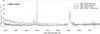 |
Fig. 7. Comparison of the reddened bright-state spectrum with the directly fitted dim-state spectrum for the CLQ J0823+4220. The dim- (grey curve) and bright-state (green curve) observed spectra are shown. We reddened the fitted components (as per Sect. 3.4.3) of the bright-state spectrum to fit the dim-state spectrum. This produced the red, dashed curve with a best-fit E(B − V) = 0.176. We also show the spectral components fitted directly to the dim-state spectrum as the blue, dashed curve for comparison. |
Fitted E(B − V) values for the Calzetti extinction curve applied to the bright-state spectra of the six CLQs.
The spectral changes in five of the six objects in our sample are fitted well by changes in obscuration, in conflict with other CLQ searches (Ruan et al. 2016; Runnoe et al. 2016; MacLeod et al. 2016, 2019). This might indicate an inherent difference in the lower luminosity sources found using our search method.
While the spectral changes are well fitted by variable obscuration, the timescales of the observed also need to be explained. LaMassa et al. (2015) analysed dust obscuration as a source of changing-look behaviour and reject this explanation due to the time scales of the variations. The crossing timescale for a dust cloud, tcross, is given by:
 (2)
(2)
with rorb the orbital radius in light-days, rsrc the orbital radius of the source and MBH the black hole mass. For sources studied by LaMassa et al. (2015), this is ∼10–20 years, an order of magnitude higher than the observed variability timescales. Runnoe et al. (2016) also found similar discrepancies in the timescales.
Using black holes masses from Sect. 3.5 and assuming an obscurer just outside the BLR with a radius calculated from the luminosity using (Bentz et al. 2009), we get a crossing time as low as ∼3 years, consistent with our objects. However, for the orbital radii consistent with the same timescale, any obscurer would have to have a size comparable to the BLR to explain the observed behaviour, if the obscurer is located at a larger radius, the timescale increases.
Therefore we conclude that for our objects, while obscuration reproduces the changes in spectral shape observed, the timescales of the observed changing-look behaviour remain difficult to explain. Changes in accretion rate are more likely to be the cause for the changing-look behaviour.
5. Conclusions
In this paper, we used repeat spectra of 24 782 extra-galactic objects in SDSS-II (Abazajian et al. 2009) to search for CLQs with variability levels weaker than those detected in previous studies. We selected all sources that show weakening or strengthening of continuum emission bluewards of 4000Åas well as disappearance or appearance of the Hβ or Hα broad emission lines between SDSS epochs. As a result, we detected six CLQs, four of which are newly discovered here.
By detecting new CLQs in a previously well-studied spectrometric dataset, we have shown that using direct comparison between repeat spectra is effective for detecting CLQs. Furthermore, the method can be used to identify CLQs that lie below the detection threshold of methods that rely on pre-selection either by photometric variability or change of spectral type in pipeline classifications.
Our other findings can be summarised as follows. Firstly, the six CLQs have redshifts 0.1 ⩽ z ⩽ 0.3. Two show transitions with disappearing, three with appearing, and one both disappearing and re-appearing broad emission lines. The CLQ J1723+5504 transitioned from an intermediate type 1.8 AGN to a type 1 AGN in 184 days (142 in the rest frame); the fastest observed changing-look behaviour in a distant AGN with quasar luminosity.
Secondly, we decomposed the CLQ spectra by fitting galaxy templates, a power law continuum as well as broad and narrow line emission. The difference spectrum of all six CLQs was well fitted by disc emission slightly shallower than the standard fυ ∝ υ1/3 accretion disc model, in agreement with previous studies (Ruan et al. 2014).
Thirdly, the CLQs have black hole masses in the range 3 × 10⁷ to 4 × 10⁸ M⊙ and Eddington ratios Lbol/LEdd ∼ 0.002 − 0.03, making these moderately luminous AGN (Lbol ∼ 1043 − 44 erg s−1). Therefore, the CLQs are hosted by massive black holes with accretion well below the Eddington limit.
Fourthly, the narrow line ratios for five of the six CLQs are indicative of ionisation by an AGN. Only one object shows a mixture of star formation and AGN activity as the source of ionisation. This indicates that the ionising radiation in CLQs was dominated by AGN over the last > 103 − 4 years. This supports that even turning on CLQs have experienced flickering in the past, rather than turning on over the past years.
Finally, we showed that the changes in spectral shape are explained by changes in accretion rate as well as changes in obscuration. An obscuration origin is unlikely due to the short timescales on which transitions are observed. Therefore, changes in accretion rate are the likely the cause of the changing-look behaviour in our sample. A complete disappearance of the BLR as predicted (Elitzur & Ho 2009) by models is not favoured, however, our data is consistent with a switch in the accretion state, as predicted by Noda & Done (2018).
We have shown that using difference spectra can be used to detect CLQs not detected by photometric variability and therefore represents an additional method for CLQ searches. Using the method presented here, we detected CLQs an order of magnitude fainter than those detected in photometric searches and we reached higher completeness than spectroscopic searches relying on a change of object type in the pipeline classification.
More data will be needed to identify the physical processes that drive changing-look behaviour at the low luminosity end. Further research is also needed to determine if all CLQs are driven by the same physical process.
We define the term quasar luminosity to mean bolometric luminosity ⩽1044 erg s−1.
All threshold values were optimised before searching the entire super-set using a subset of 184 objects whose SDSS pipeline classification changed between GALAXY and QSO across at least two epochs. Thresholds were chosen so that the algorithm selected 38 objects of interest for visual inspection from said subset.
Type 1.5 objects are defined as intermediate between type 1 and type 2 with easily apparent broad Hβ emission. type 1.8 is intermediate between type 1.5 and type 2, with a weaker Hβ than type 1.5 yet still visible (Osterbrock 1977).
With the exception of the BOSS spectrum of J0002-0027.
The BOSS spectrum of J0002-0027 was fitted independently from its earlier epoch spectra as it was observed with a 2″ fibre rather than a 3″ fibre, so we expected a weaker galaxy contribution to the narrow emission (as explained in Sect. 3.4.2).
Acknowledgments
We thank the anonymous referee for helpful comments. We acknowledge Benjamin Pickford for his contribution to developing the sample selection method and confirming the six CLQs in the sample. Funding for the SDSS and SDSS-II has been provided by the Alfred P. Sloan Foundation, the Participating Institutions, the National Science Foundation, the US Department of Energy, the National Aeronautics and Space Administration, the Japanese Monbukagakusho, the Max Planck Society, and the Higher Education Funding Council for England. The SDSS Web Site is http://www.sdss.org/. The SDSS is managed by the Astrophysical Research Consortium for the Participating Institutions. The Participating Institutions are the American Museum of Natural History, Astrophysical Institute Potsdam, University of Basel, University of Cambridge, Case Western Reserve University, University of Chicago, Drexel University, Fermilab, the Institute for Advanced Study, the Japan Participation Group, Johns Hopkins University, the Joint Institute for Nuclear Astrophysics, the Kavli Institute for Particle Astrophysics and Cosmology, the Korean Scientist Group, the Chinese Academy of Sciences (LAMOST), Los Alamos National Laboratory, the Max-Planck-Institute for Astronomy (MPIA), the Max-Planck-Institute for Astrophysics (MPA), New Mexico State University, Ohio State University, University of Pittsburgh, University of Portsmouth, Princeton University, the United States Naval Observatory, and the University of Washington.
References
- Abazajian, K. N., Adelman-McCarthy, J. K., Agueros, M. A., et al. 2009, ApJ, 182, 543 [Google Scholar]
- Antonucci, R. 1993, ARA&A, 31, 473 [Google Scholar]
- Antonucci, R., & Cohen, R. D. 1983, ApJ, 271, 564 [Google Scholar]
- Baldwin, J. A., & Phillips, M. M. 1981, PASP, 93, 5 [Google Scholar]
- Bentz, M. C., Peterson, B. M., Netzer, H., Pogge, R. W., & Vestergaard, M. 2009, ApJ, 697, 160 [Google Scholar]
- Brinchmann, J., Charlot, S., White, S. D. M., et al. 2004, MNRAS, 351, 1151 [NASA ADS] [CrossRef] [Google Scholar]
- Calzetti, D., Armus, L., Bohlin, R. C., et al. 2000, ApJ, 533, 682 [NASA ADS] [CrossRef] [Google Scholar]
- Dexter, J., & Agol, E. 2011, ApJ, 727, L24 [Google Scholar]
- Elitzur, M., & Ho, L. C. 2009, ApJ, 701, L91 [Google Scholar]
- Elitzur, M., Ho, L. C., & Trump, J. R. 2014, MNRAS, 438, 3340 [Google Scholar]
- Eracleous, M., Livio, M., & Binette, L. 1995, ApJ, 445, L1 [Google Scholar]
- Fitzpatrick, E. L. 1999, PASP, 111, 63 [NASA ADS] [CrossRef] [Google Scholar]
- Gezari, S., Martin, D. C., Milliard, B., et al. 2006, ApJ, 653, L25 [Google Scholar]
- Gezari, S., Heckman, T., Cenko, S. B., et al. 2009, ApJ, 698, 1367 [NASA ADS] [CrossRef] [Google Scholar]
- Gezari, S., Chornock, R., Rest, A., et al. 2012, Nature, 485, 217 [NASA ADS] [CrossRef] [PubMed] [Google Scholar]
- Gezari, S., Hung, T., Cenko, S. B., et al. 2017, ApJ, 835, 144 [Google Scholar]
- Greene, J. E., Peng, C. Y., & Ludwig, R. R. 2010, ApJ, 709, 937 [Google Scholar]
- Hall, P. B., Sarrouh, G. T., & Horne, K. 2018, ApJ, 854, 93 [Google Scholar]
- Hao, L., Strauss, M. A., Tremonti, C. A., et al. 2005, AJ, 129, 1783 [Google Scholar]
- Kauffmann, G., Heckman, T. M., Tremonti, C., et al. 2003, MNRAS, 346, 1055 [Google Scholar]
- Kewley, L. J., Groves, B., Kauffmann, G., & Heckman, T. 2006, MNRAS, 372, 961 [NASA ADS] [CrossRef] [Google Scholar]
- LaMassa, S. M., Cales, S., Moran, E. C., et al. 2015, ApJ, 800, 10 [Google Scholar]
- Lyutyi, V. M., Oknyanskii, V. L., & Chuvaev, K. K. 1984, Sov. Astron. Lett., 10, 335 [Google Scholar]
- MacLeod, C. L., Ivezić, Ž., Kochanek, C. S., et al. 2010, ApJ, 721, 1014 [Google Scholar]
- MacLeod, C. L., Ross, N. P., Lawrence, A., et al. 2016, MNRAS, 457, 389 [Google Scholar]
- MacLeod, C. L., Green, P. J., Anderson, S. F., et al. 2019, ApJ, 874, 8 [Google Scholar]
- Merloni, A., Dwelly, T., Salvato, M., et al. 2015, MNRAS, 452, 69 [NASA ADS] [CrossRef] [Google Scholar]
- Nenkova, M., Sirocky, M. M., Nikutta, R., Ivezic, Z., & Elitzur, M. 2008, ApJ, 685, 160 [Google Scholar]
- Noda, H., & Done, C. 2018, MNRAS, 480, 3898 [NASA ADS] [CrossRef] [Google Scholar]
- Osterbrock, D. E. 1977, ApJ, 215, 733 [Google Scholar]
- Penston, M. V., & Perez, E. 1984, MNRAS, 211, P33 [Google Scholar]
- Richards, G. T., Hall, P. B., Vanden Berk, D. E., et al. 2003, AJ, 126, P1131 [Google Scholar]
- Ross, N. P., Saavik Ford, K. E., Graham, M., et al. 2018, MNRAS, 480, 4468 [Google Scholar]
- Ruan, J. J., Anderson, S. F., Dexter, J., & Agol, E. 2014, ApJ, 783, 105 [Google Scholar]
- Ruan, J. J., Anderson, S. F., Cales, S. L., et al. 2016, ApJ, 826 [Google Scholar]
- Runnoe, J. C., Brotherton, M. S., & Shang, Z. H. 2012, MNRAS, 422, 478 [Google Scholar]
- Runnoe, J. C., Cales, S., Ruan, J. J., et al. 2016, MNRAS, 455, 1691 [Google Scholar]
- Schawinski, K., Thomas, D., Sarzi, M., et al. 2007, MNRAS, 382, 1415 [NASA ADS] [CrossRef] [Google Scholar]
- Schlegel, D. J., Finkbeiner, D. P., & Davis, M. 1998, ApJ, 500, 525 [NASA ADS] [CrossRef] [Google Scholar]
- Schmidt, K. B., Rix, H. W., Shields, J. C., et al. 2012, ApJ, 744, 147 [Google Scholar]
- Shakura, N. I., & Sunyaev, R. A. 1973, A&A, 24, 337 [NASA ADS] [Google Scholar]
- Shapovalova, A. I., Popovic, L. C., Burenkov, A. N., et al. 2010, A&A, 509, A106 [NASA ADS] [CrossRef] [EDP Sciences] [Google Scholar]
- Stern, D., McKernan, B., Graham, M. J., et al. 2018, ApJ, 864, 27 [Google Scholar]
- Stoughton, C., Lupton, R. H., Bernardi, M., et al. 2002, AJ, 123, 485 [Google Scholar]
- Urry, C. M., & Padovani, P. 1995, PASP, 107, 803 [Google Scholar]
- Vanden Berk, D. E., Wilhite, B. C., Kron, R. G., et al. 2004, ApJ, 601, 692 [Google Scholar]
- Vanden Berk, D. E., Shen, J. J., Yip, C. W., et al. 2006, AJ, 131, 84 [Google Scholar]
- Veilleux, S. 1991, ApJ, 369, 331 [Google Scholar]
- Wilhite, B. C., Vanden Berk, D. E., Kron, R. G., et al. 2005, ApJ, 633, 638 [Google Scholar]
- Yang, Q., Wu, X.-B., Fan, X., et al. 2018, ApJ, 862, 109 [Google Scholar]
- Yip, C. W., Connolly, A. J., Szalay, A. S., et al. 2004a, AJ, 128, 585 [Google Scholar]
- Yip, C. W., Connolly, A. J., Vanden Berk, D. E., et al. 2004b, AJ, 128, 2603 [Google Scholar]
- York, D. G., Adelman, J., Anderson, J. E., et al. 2000, AJ, 120, 1579 [CrossRef] [Google Scholar]
All Tables
Fitted E(B − V) values for the Calzetti extinction curve applied to the bright-state spectra of the six CLQs.
All Figures
|
Fig. 1. Observed spectra and the difference spectrum of the turning off CLQs. The quasars shown are J0823+4220 (top two panels), and J0126–0839 (bottom two panels). Upper: the observed optical spectra, with the first epoch (black) and second epoch (red) both shown. Lower: the difference spectrum |Δfλ| (black) is shown, demonstrating how the CLQs were identified, and the resemblance of the variable component to an accretion disc. A fitted Shakura-Sunyaev accretion disc power law fυ ∝ υ1/3 (dashed-blue) and a best-fit power law to the continuum (orange) is shown. |
| In the text | |
|
Fig. 2. Observed spectra and the difference spectrum of the turning on CLQs. The turning on CLQs are shown in the same format as Fig. 1. The quasars shown are J1723+5504 (top two panels), J0829+4154 (middle two panels), and J1358+4934 (bottom two panels). |
| In the text | |
|
Fig. 3. Observed spectra and the difference spectra of the turning off and on CLQ J0002-0027. Top: the three observed spectra, including the extra BOSS spectrum (blue curve), are shown in the SDSS Legacy rest wavelength range of the object. The epochs for the black, red, and blue spectra are MJD = 51791, 52559, and 55477, respectively. Middle: the difference spectra of the first and second epoch (black curve), and the second and third epoch (red) are shown on the same flux scale, with a constant added to the latter. Bottom: a zoomed in view of the observed spectra in the Hβ (left) and Hα (right) regions is shown. |
| In the text | |
|
Fig. 4. Spectral decomposition of the CLQ J0823+4220, which turned off. The fitted galaxy (blue curve) and quasar (green) components, and their sum (red) from the best-fit eigenspectrum coefficients (found as per Sect. 3.4.2) are shown. Top: the earlier epoch (MJD = 52266) bright-state spectrum. Bottom: the later epoch (MJD = 54524) dim-state spectrum. |
| In the text | |
|
Fig. 5. Emission line fitting to the decomposed AGN spectrum (black) of the CLQ J0823+4220. The AGN spectrum was fitted (red) with a power law continuum (green) and a selection of narrow and broad Gaussians. The fitting procedure is described in Sect. 3.4.3. |
| In the text | |
|
Fig. 6. BPT diagram showing the narrow emission line ratios of the six CLQs, three turning on (cross) and two turning off (star), and one turning off then on (plus). The heat map was produced using the MPA-JHU emission line analysis of 927 552 DR7 objects, thereby showing the overall SDSS trend (Brinchmann et al. 2004). Three emission line classification schemes are shown. Kauffmann et al. (2003) (dashed line) separates star-forming and composite host galaxies, Kewley et al. (2006) (dotted line) separates AGN and composite host galaxies, and Schawinski et al. (2007) separates LINERs from AGN. |
| In the text | |
|
Fig. 7. Comparison of the reddened bright-state spectrum with the directly fitted dim-state spectrum for the CLQ J0823+4220. The dim- (grey curve) and bright-state (green curve) observed spectra are shown. We reddened the fitted components (as per Sect. 3.4.3) of the bright-state spectrum to fit the dim-state spectrum. This produced the red, dashed curve with a best-fit E(B − V) = 0.176. We also show the spectral components fitted directly to the dim-state spectrum as the blue, dashed curve for comparison. |
| In the text | |
Current usage metrics show cumulative count of Article Views (full-text article views including HTML views, PDF and ePub downloads, according to the available data) and Abstracts Views on Vision4Press platform.
Data correspond to usage on the plateform after 2015. The current usage metrics is available 48-96 hours after online publication and is updated daily on week days.
Initial download of the metrics may take a while.