| Issue |
A&A
Volume 650, June 2021
|
|
|---|---|---|
| Article Number | A96 | |
| Number of page(s) | 10 | |
| Section | Stellar structure and evolution | |
| DOI | https://doi.org/10.1051/0004-6361/202039970 | |
| Published online | 11 June 2021 | |
Non-synchronous rotations in massive binary systems
II. The case of HD 96264A⋆
1
Instituto de Astrofísica de La Plata, CONICET–UNLP, Paseo del Bosque s/n, B1900FWA La Plata, Argentina
e-mail: This email address is being protected from spambots. You need JavaScript enabled to view it.
2
Facultad de Ciencias Astronómicas y Geofísicas, Universidad Nacional de La Plata, La Plata, Argentina
3
Las Campanas Observatory, Carnegie Observatories, Casilla 601, La Serena, Chile
4
Departamento de Astronomía, Universidad de La Serena, Av. Cisternas 1200 Norte, La Serena, Chile
Received:
23
November
2020
Accepted:
6
March
2021
Abstract
Context. The OWN Survey has detected several O-type stars with composite spectra whose individual components show very different line broadening. Some of these stars have been revealed as binary systems whose components are asynchronous. This fact may be related to the processes acting in these systems (e.g., angular-momentum transfer, tidal forces, etc.) or to the origin of the binaries themselves.
Aims. We aim to determine the orbital and physical parameters of the massive star HD 96264A in order to confirm its binary nature and to constrain the evolutionary status of its stellar components.
Methods. We computed the spectroscopic orbit of the system based on the radial velocity analysis of 37 high-resolution, high-S/N, multi-epoch optical spectra. We disentangled the composite spectrum and determined the physical properties of the individual stellar components using FASTWIND models incorporated to the IACOB-GBAT tool. We also computed a set of evolutionary models to estimate the age of the system and explore its tidal evolution.
Results. HD 96264A is a binary system composed of an O9.2 IV primary and a B0 V(n) secondary, with minimum masses of 15.0 ± 0.5 M⊙ and 9.9 ± 0.4 M⊙, respectively, in a wide and eccentric orbit (P = 124.336 ± 0.008 d; e = 0.265 ± 0.005). The primary and secondary components have different projected rotational velocities (∼40 and ∼215 km s−1 respectively), and the physical properties derived through quantitative spectroscopic analyses include masses of ∼20.5 M⊙ and 16.8 M⊙, respectively. The evolutionary models indicate an approximate age of 4.5 Myr for both stars in the pair, corresponding to current masses and radii of 26.0 M⊙ and 10.8 R⊙ for the primary, and 17.9 M⊙ and 7.0 R⊙ for the secondary.
Conclusions. The youth and wide orbit of the system indicate that the non-synchronous rotational nature of its components is a consequence of the stellar formation process rather than tidal evolution. This circumstance should be accounted for in theories of binary star formation.
Key words: binaries: spectroscopic / stars: rotation / stars: early-type / stars: individual: HD 96264A
Based on data acquired at Complejo Astronómico El Leoncito, operated under agreement between the Consejo Nacional de Investigaciones Científicas y Técnicas de la República Argentina and the National Universities of La Plata, Córdoba and San Juan. Also based on observations gathered at Las Campanas (Carnegie Observatories) and ESO-La Silla Observatory.
© ESO 2021
1. Introduction
Massive stars are among the most important and challenging objects in the Universe. They are thought to be the progenitors of several types of supernovae, and the origin of other phenomena such as gamma-ray bursts and the recently observed gravitational waves. Our understanding about how these stars form, live and die is not clear yet. Improving our knowledge requires the determination of stellar parameters such as masses and radii in as many objects as possible. Binary systems provide the best way to determine these fundamental parameters and are therefore considered as key targets for improving our knowledge of massive stars.
In the last years, it has been proved that a high percentage of massive stars belong to binary or multiple systems (Mason et al. 1998; Bosch & Meza 2001; Sana & Evans 2011; Duchêne & Kraus 2013; Sana 2017; Barbá et al. 2017). The nearby companion affects the evolution of each component in the system (Sana et al. 2012) by means of processes such as tidal forces and mass and angular momentum exchange. The efficiency of these phenomena is not well understood and constitutes one of the largest uncertainties in binary evolution. Moreover, during mass transfer, the mass gainer can spin up in a manner that is not well understood (Wellstein et al. 2001; Petrovic et al. 2005; de Mink et al. 2013).
The spectroscopic monitoring of Southern Galactic O and WN stars, that is, the OWN Survey (Barbá et al. 2010, 2014, 2017), is a program that aims to observe, with high-resolution optical spectroscopy, a sample of Southern O- and WN-type stars for which the multiplicity status is unknown. One of the results of this survey has been the identification of several double-lined spectroscopic binaries (SB2) showing line profiles indicative of different projected rotational velocities for each component. This means that either the components rotate at different velocities or their spin axes are not aligned, i.e. are asynchronous. These SB2 stars form the sample studied in this series of papers.
The first paper of this series refers to HD 93343, a previously known binary system. Putkuri et al. (2018) determined for the first time the radial velocity (RV) orbital solution for both stars in the binary. From a quantitative analysis of the spectrum of each component, these authors obtained very different projected rotational velocities of 63 ± 5 and 325 ± 50 km s−1, respectively. Considering the youth of the system and the width of the orbit, it was concluded that the rotational configuration should be intrinsic to the birth of the system. We aim carry out the same analysis of the whole sample of SB2 stars, with the goal being to contribute observational constraints to theories of massive star formation. In this context, we would like to point out the recently published discovery of a massive protobinary, IRAS 07299-1651, observed at the 1.3 mm continuum and H30α recombination emission line with ALMA by Zhang et al. (2019). These latter authors identified a pair of protostars embedded in the common disc and detected a misalignment between the circumbinary and circumstellar discs indicative of different angular momentum directions.
In the present (second) paper of the series, we present the analysis of HD 96264A (CPD −60 2505; RA(J2000) =  ; Dec(J2000) = −61° 03′05
 8; V = 7.62 mag) a star considered to be the brightest member of the Lodén 306 open cluster (Lodén 1980) at a distance of 1.83 kpc (Carraro et al. 2017). We note that the individual distance to HD 96264A was calculated by Bailer-Jones et al. (2018) as 2915
 pc. We discuss this issue below.
HD 96264A is an astrometric binary (WDS J11049-6103A; Mason et al. 2001) and its companion HIP 54171 (WDS J11049-6103B), a B4 V-type star (Lindroos 1985), is reported at about 24 arcsec (Mason et al. 1998). Also, it is an SB2 according to OWN data and was classified as the first standard O9.5 III type star by Sota et al. (2011). After the star was found to be an SB2, its spectrum was revised by Sota et al. (2014); these authors did not see double lines at the R 2500 resolving power of the Galactic O-Star Spectroscopic Survey (GOSSS), and therefore they kept the object as standard. Information about its RV was presented in early works (Martin 1967; Thackeray et al. 1973; Conti et al. 1977) but only Thackeray et al. (1973) indicated variability. Chini et al. (2012) identified this star as a SB2 but no orbit or RVs were provided in that work.
Here, we present the first RV orbital solution, a quantitative spectroscopic analysis, and we discuss the evolutionary status of HD 96264A. The paper is organised as follows: Sect. 2 describes the spectroscopic dataset; Sect. 3 explains the method used to obtain the individual spectrum of each component and the RV measurements; Sect. 4 presents the determination of the RV orbital solution; Sect. 5 includes the spectroscopic analysis (the spectral classification and the determination of stellar parameters for each component); Sect. 6 shows an analysis of the evolutionary status of HD 96264A. Finally, in the Sect. 7 we summarise our conclusions.
2. Observations
Our observational dataset consists of 37 high-resolution spectra acquired between 2008 and 2019. We employed the échelle spectrographs attached to the 2.15 m J. Sahade telescope at Complejo Astronómico El Leoncito (CASLEO), Argentina; the 2.5 m Irénée du Pont telescope at Las Campanas Observatory (LCO), Chile; and the MPG/ESO 2.2 m telescope at La Silla Observatory, Chile. Table 1 gives details of the instrumental configurations used in this work. There, the observatory and instrument identification, the time-span of each dataset, the spectral coverage, the resolving power (R), and the number of collected spectra (n) are given in successive columns.
Details of the instrumental configurations.
As spectrographs at CASLEO and LCO are attached to the telescope, we obtained comparison lamp spectra of Th-Ar, immediately after or before each target integration, at the same position. CASLEO and LCO spectra were processed using the standard IRAF1 routines. FEROS data were reduced through the standard reduction pipeline layered in the MIDAS package provided by the European Southern Observatory. In Fig. 1 we show two normalised LCO spectra of the binary near both quadratures. The box in the upper right-hand corner shows the He Iλ5876 line at different phases to illustrate the contrast between both components of the binary.
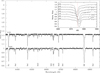 |
Fig. 1. Section of the LCO spectra of HD 96264A obtained near both quadratures. The upper box on the right side of the figure shows LCO and ESO spectra in the region of He Iλ5876 obtained at different orbital phases in order to illustrate the observed variation in the line profile. The phases of the different observations, according to the ephemerides of Table 2, are indicated above the correspondent spectrum. |
3. Spectral disentangling and radial velocity measurements
We employed a method for separating composite spectra based on the code published by González & Levato (2006). This code consists in combining the composite (A+B) spectra shifted to the RV of one of the components (e.g. A). This combined spectrum, namely A+(B), contains the features of component A but component B features are diluted because they are at different RVs. Subsequently, this A+(B) spectrum was subtracted from each A+B (shifted to the same RV of A) to obtain the spectrum of B-(B), which was shifted to the B component RVs and combined to obtain an almost pure component B spectrum. As this first iteration needs an initial RV for each component, we attempted preliminary measurements of some He I and He II lines using the task deblend available in the IRAF SPLOT package. We start the procedure of separating composite spectra using those spectra that show the largest RV separation between components (i.e ideally observed during quadratures). Once the initial templates are generated, the code determines the RVs cross-correlating each template (A or B) with the subtraction of the other template from the composite spectra (A+B – B or A+B – A). As these new RVs are expected to be more accurate than those initially estimated, the next new templates tend to minimise the residuals of the other component. After a few iterations the method converges to almost pure spectra of each component, and the RVs are representative of each component as well. The remarkable feature of these systems, that is, the broad and narrow line components, forced us to consider some variations to the method (see Putkuri et al. 2018, for further details). The most important change was the construction of a primary component template using the IACOB Grid-Based Automatic Tool (IACOB-GBAT)2, which was then subtracted from a composite one to obtain an initial template for the secondary.
The cross-correlation was performed in different spectral ranges, each of them 10 Åin width, taken around the following spectral lines: He Iλλ4026, 4471, 5015, 5876 Åand He IIλλ4686, 5411 Åfor the narrow component, and He Iλλ5015, 5876 Åand He IIλ4686 Åfor the broad one whenever it was measurable. The very broad shape of the secondary lines made RV measurements particularly difficult, especially for He Iλ5876 which is also affected by telluric absorptions. For that reason we were not always able to obtain a reliable RV for this line. The final RVs used in the orbital solution are shown in Table 2.
Radial velocity measurements (km s−1) of both components in the HD 96264A system.
We searched for systematic errors between the different spectrographs by measuring RVs for the Na I D doublet. The spectra taken at LCO and La Silla display multiple components from which the strongest and broadest is observed at −8.3 km s−1, with a strong satellite line at +10 km s−1, and two fainter components at −18.9 km s−1 (barely resolved) and +29.4 km s−1, respectively. These components are unresolved in CASLEO spectra. To carry out the comparison between the different spectrographs we measured RVs from the integrated line profile obtaining −3.1 ± 1.8 km s−1, −4.0 ± 0.7 km s−1 and −3.8 ± 0.2 km s−1 for Sahade/REOSC, du Pont/échelle, and 2p2/FEROS, respectively. Given that these values are within the error intervals, we did not correct for any systematic differences between the three spectrographs.
In addition, we made several measurement attempts on the same line to obtain an error estimation for stellar absorption lines, finding differences of around 3 km s−1. In the case of the broader component, because of the uncertainty in the adjustment of the line centres, we considered that the RVs for this component present an error of ∼10 km s−1 (see Putkuri et al. 2018).
4. Orbital solution
We searched for periodicities in the RVs using the interactive NASA Exoplanet Archive Periodogram Service employing the Lomb-Scargle method (Scargle 1982). We obtained a most probable period of P = 123.9 ± 2.9 days. In Fig. 2 we show the resulting periodogram where it can be noted that the period determination is robust and no conspicuous aliases are present. With this P as initial value, we determined the RV orbital solution simultaneously for both components by means of the GBART code3. The CASLEO RVs were given half weight as CASLEO spectra have lower resolution than those obtained at LCO and La Silla. The derived orbital parameters are given in Table 3 as follows: period (P), time of periastron passage (Tperi), systemic velocity (V0), eccentricity (e), longitude of periastron (ω), semiamplitude of each relative orbit (Ki), major semiaxis (ai sin i), minimum mass (Mi sin3i), and mass ratio (q). The RV curves are illustrated in Fig. 3 along with the observations and their residuals with respect to the model.
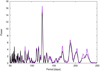 |
Fig. 2. Periodograms of the primary RVs obtained with the NASA Exoplanet Archive Periodogram Service. In black, the OWN Survey dataset; in violet, the OWN Survey dataset plus five RVs gathered from the literature. |
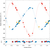 |
Fig. 3. RV curves of the primary (blue) and secondary (red) components of the binary system HD 96264A calculated with the parameters of the orbital solution shown in Table 3 along with the observations. Errors on primary RVs are smaller than the symbol sizes. Filled circles represent LCO and La Silla data, and open circles are used for CASLEO. Yellow circles represent the previously published RVs. The O-C for the primary (blue) and secondary (red) are depicted in the bottom panel. |
Orbital parameters of the HD 96264A system derived from the radial velocity curve.
Although scarce in number, the RV measurements published by Thackeray et al. (1973) (4 data points) and Conti et al. (1977) (1 data point) allow us to extend the time coverage to almost 50 years. These five RVs, assigned to the narrow component, fit our orbital solution acceptably (added in yellow in Fig. 3) and the period is better constrained as a consequence of the longer time baseline, as shown in Fig. 2 (violet line). It is noticeable that Martin (1967) published a RV of −64 km s−1, but unfortunately no date for that measurement is given.
5. Spectroscopic analysis
5.1. Spectral classification
HD 96264A is the spectral classification standard of the O9.5 III subtype stars (Sota et al. 2011, 2014). In this work, we analyse the disentangled spectrum of the narrow primary component, from now on called HD 96264Aa, comparing it with the adjoining standard stars in order to evaluate the contribution of its companion. Considering the ratios He IIλ4542/He Iλ4388 and He IIλ4200/He Iλ4144, which are slightly less than unity, and Si IIIλ4552/He IIλ4542 which is even smaller, we find a spectral type of O9.2, while the comparison of the Si IVλλ4089 and 4116 with He I/He IIλ4026 and He Iλ4121 indicates a luminosity class IV. Thus the spectral type determined corresponds to O9.2 IV.
The spectral classification of the secondary component, HD 96264Ab, is a more challenging task. This is due to the lower signal-to-noise ratio (S/N) obtained for the disentangled spectrum for that component. We relied on some spectra obtained during quadratures instead. In those spectra, the presence of He Iλ4471 can be clearly noted, along with He IIλ4542, albeit rather marginal. Similarly, we can see He Iλ4144 and faint He IIλ4200. This is indicative of a spectral type around O9.7 or B0. To assess the luminosity class, we analysed the relation between the intensities of He IIλ4686 and He Iλ4713 and between Si IVλ4089 and He Iλ4026. From these intensity ratios we infer a luminosity class of V. The qualifier ‘(n)’ is added to account for the broadening of the spectral features, pointing to v sin i ≥ 200 km s−1 (Sota et al. 2011).
The disentangled spectra are shown in Fig. 4 in the wavelength region of the optical classification.
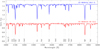 |
Fig. 4. Normalised disentangled spectra of the primary (shifted upwards by 0.42 continuum units) and secondary components of HD 96264A system. Relevant features for spectral classification are indicated. Some artefacts on the spectra, mostly seen in the wings of the hydrogen lines, are originated in the disentangling process. |
5.2. Quantitative spectroscopic analysis
We employed the IACOB-BROAD tool (Simón-Díaz et al. 2011; Simón-Díaz & Herrero 2014) and the IACOB Grid-Based Automatic Tool (IACOB-GBAT) to obtain estimates of the rotational and macroturbulence broadening as well as physical stellar parameters such as the effective temperature (Teff) and the stellar surface gravity (log g).
5.2.1. Line broadening
The IACOB-BROAD tool combines the Fourier Transform (FT) and the goodness-of-fit (GOF) technique to characterise the broadening of the spectral lines of each component. The GOF technique allows a complete characterisation of the line broadening in terms of projected rotational and macroturbulence velocities (v sin i, vmac), based on a simple line-profile fitting in which an intrinsic profile is convolved with various line-broadening profiles and compared with the observed profile using a χ2 formalism (see application of the method in Ryans et al. 2002). The FT technique estimates the v sin i of the line by means of the identification of the first zero in the Fourier space (see Simón-Díaz & Herrero 2007).
The v sin i and vmac of each component were obtained fitting O IIIλ5592 from the primary template and He Iλλ4713, 4471, 4922, and 5015 from the secondary one. We decided to use these lines because the O III line is not distinguishable in the secondary component template and moreover the He I lines are only slightly affected by the Stark effect as has been demonstrated by Dimitrijevic & Sahal-Brechot (1990) and also later by Simón-Díaz & Herrero (2007) using a sample of about 50 OB stars.
We obtained v sin i = 39 ± 2 km s−1 and vmac = 55 ± 2 km s−1 for the primary component (see Fig. 5). Simón-Díaz & Herrero (2014) showed that the broadening values of ≤40 km s−1, considered as the lower velocity regime, must be regarded as an upper limit on the actual broadening of the lines because the microturbulence could be an important effect here. This fact tends to produce overestimates of v sin i, and, in addition, the vmac value may be wholly produced by microturbulence. In this respect, we do not strictly consider v sin i = 39 km s−1 to be the v sin i value of the primary star, but rather its upper limit.
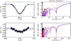 |
Fig. 5. Graphical output of the IACOB-BROAD tool for both stellar components of HD 96264A. The left upper panel shows the line profile of O IIIλ5592 of the primary component and the right upper panel shows its Fourier transform. The bottom panels show similar plots for the He Iλ5015 line of the secondary component. Four fits are presented in each case: v sin i(FT) in red, (v sin i, vmac) (GOF) in blue, (v sin i, vmac = 0.0) (GOF) in green, and (v sin i = FT, vmac) (GOF) in violet. |
For the secondary, the four fitted lines gave similar results, and therefore we adopted their average, v sin i = 215 ± 11 km s−1. In Fig. 5 we show the IACOB-BROAD fit for both components. From this figure it is clear that the fit obtained for the secondary star without macroturbulence (vmac = 0 km s−1; green line) is as good as the fit with macroturbulence (vmac = 58 km s−1; violet line).
Simón-Díaz & Herrero (2014) explained that in stars with v sin i higher than 150 km s−1 the effect of noise, blending, and continuum normalisation becomes significant. Above a certain value of v sin i, the effect of the additional broadening only results in a subtle shaping of the extended wings. For this, we were not able to obtain a reliable estimate for vmac. Consequently, vmac = 58 ± 11 km s−1 should be considered as an upper limit.
To verify the projected rotational velocity obtained for the secondary component, HD 96264Ab, we tried other methods based on the calibration of the FWHM of He Iλλ4026, 4388 and 4471 (Daflon et al. 2007) and its modification proposed by Ferrero (2016) using He Iλλ4713 and 5015. We obtained very similar values for the primary star and v sin i = 200 km s−1 for the secondary star, validating the results obtained by means of IACOB-BROAD.
The rotational broadening of the HD 96264Aa was also determined by Holgado et al. (2018) who obtained v sin i = 29 km s−1 and vmac = 65 km s−1. The difference with our values could arise from the fact that their analysis does not consider the secondary contribution. Furthermore, the spectrum they used was obtained near quadrature. Without resolving the composite spectra, the presence of the broad component leads to an overestimation of vmac and an underestimation of v sin i.
5.2.2. Stellar parameters
We proceeded to the determination of the effective temperature and the surface gravity performing a quantitative spectroscopic analysis of the individual disentangled spectra with IACOB-GBAT (Simón-Díaz et al. 2011; Sabín-Sanjulián et al. 2014; Holgado et al. 2017, 2018). This latter is a user-friendly IDL package based on standard techniques for the quantitative spectroscopic analysis of O stars, which has been automated by applying a χ2 algorithm to a large grid of precomputed FASTWIND models (Santolaya-Rey et al. 1997; Puls et al. 2005; Rivero González et al. 2012). This tool compares observed and synthetic H and He I,II optical line profiles, which are commonly assumed to be a diagnosis for the determination of stellar parameters of O stars (Herrero et al. 1992, 2002; Repolust et al. 2004).
The following lines were used for the primary component: Hβ, Hγ, Hδ and Hϵ; He I/IIλ4026, He Iλλ4143, 4387, 4471, 4713, 4922, 5015, 5047, 5876 and 6678; He IIλλ4200, 4542, 4686, and 5411. Figure 6 shows the best fit obtained for this component, which corresponds to the model of Teff = 33 000 K and log g = 3.7 dex. In the case of the secondary component, we used He I/IIλ4026, He Iλλ4387, 4471, 4713, 4922, 5015, 5876 and He IIλλ4200, 4541, 4686, and 5411. For this component, in Fig. 7, we present the best fit which corresponds to a model with Teff = 30 000 K and log g = 3.9 dex (see Simón-Díaz et al. 2011, for information about the ranges of values considered for the free parameters in the FASTWIND grid).
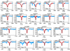 |
Fig. 6. Template of the narrow component of HD 96264A overplotted on the best fit from the IACOB-GBAT grid (solid black lines). The v sin i and vmac employed were those previously determined. The colours correspond to the spectral regions employed in the analysis (red) and discarded (sky blue). |
As one of the more severe problems in disentangling composite spectra arises from difficulties in reconstructing the wings of H lines, principally because of the very broad profiles of the secondary component lines, the derived values of log g should be taken with caution. This parameter depends on the wings of Balmer lines which are contaminated by residuals from the disentangling process. In reality, a range of log g was obtained when adding or removing lines from the analysis. We find 3.54 < log g <3.72 dex, with convergence to the value of 3.69 dex in the best fit, for the primary component. In the secondary star the 3.9 < log g <4.0 dex range was fixed based on the spectral type determined for this component. For both stars, we adopted the broadening velocities calculated above (see Sect. 5.2.1 and Table 4). As shown in Fig. 7, despite the low S/N of the secondary template we obtain a reasonably good fit.
Parameters obtained from the spectroscopic analysis of both components of HD 96264A.
Figure 8 illustrates the best fits obtained (blue and red lines for the primary and secondary components, respectively) and one of our observed composite spectra (in grey). The combined spectrum (in sky-blue) is also overplotted for comparison. The contribution of the broad component to the combined He I lines is evident but its contribution to the He II lines is more subtle, as expected from its lower effective temperature and large v sin i. We also note the difficulty in precisely determining the surface gravity of the components from the wings of the hydrogen Balmer lines, which is due to the blending of the lines of both components.
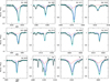 |
Fig. 8. Composite FEROS spectrum of HD 96264A (in grey) compared to a combined synthetic model (in sky blue) resulting from the best fitting FASTWIND models to each stellar component (Teff = 33 kK, log g = 3.70 dex and log Q = −12.7 for component A; Teff = 30 kK, log g = 3.90 dex and log Q = −12.7 for component B). Both individual models were diluted and added in order to obtain the composed model. All FASTWIND models in this figure have YHe = 0.09 and β = 0.8. |
The fundamental parameters, radius (R), luminosity (L), and spectroscopic mass (Msp) can be calculated by IACOB-GBAT if the absolute magnitude is known. In turn, this parameter can be obtained if the distance to the system, the interstellar absorption and the relation between the individual fluxes are known. There are several distances determined for HD 96264A. On one hand, there are those inferred from its membership to the host cluster Lodén 306, ranging from d = 1.8 kpc (Carraro et al. 2017) to d = 2.0 kpc (Kharchenko et al. 2005), depending on the value of the adopted optical total-to-selective extinction ratio RV. On the other side, there are two similar determinations: from the Gaia parallax ( pc; Bailer-Jones et al. 2018) and from the spectral-energy-distribution analysis (d = 2511 pc; Maíz Apellániz & Barbá 2018). These latter authors also estimated the optical–near-infrared (NIR) dust extinction towards the star AV ∼ 0.77 mag.
The flux relation between the binary components was evaluated through visual estimation, as follows: The templates obtained from the disentangling method were corrected by different dilution factors and compared to synthetic H, He I, and He II lines via the IACOB-GBAT. We found that a brightness ratio of 0.37 yielded the best fit for both components, meaning that approximately 73% and 27% of the total light correspond to the primary and secondary stars, respectively.
With all the available information, we obtained MV = −4.2 and −5.12 mag for the primary, and MV = −3.12 and −4.04 mag for the secondary, assuming the most extreme values of distances (1.9 and 2.9 kpc, respectively). These calculations favour the 2.5 kpc distance (intermediate value) from Maíz Apellániz & Barbá (2018)4, and therefore we adopted the MV obtained with that distance. It is interesting to note that HIP 54171 (=Gaia DR2 5337283948144897664) is at a distance of 2456 pc (Bailer-Jones et al. 2018), which supports its status as an astrometric companion of HD 96264A.
The fundamental parameters obtained, shown in Table 4, fall within the expected range of values calibrated by Martins et al. (2005), interpolating values between O9 and O9.5 spectral types and V–III luminosity class. The parameters for the O9.2 IV-type star result in R being 0.4 R⊙ bigger, log(L/L⊙) being 0.1 dex brighter, and Msp being 1.7 M⊙ greater than the values provided by Martins et al. (2005). Regarding the secondary B0 V component, its parameters can be compared with those determined by Nieva & Przybilla (2014) for HD 36512 (=υ Ori). In this case, luminosity and mass are in good agreement, but not the radius, which is 2.8 R⊙ smaller than ours. This latter parameter, in turn, is comparable with the value estimated by Cox (2000).
These fundamental parameters can also be compared with empirical determinations from eclipsing binaries as can see in Table 5. Our values for the O9.2 IV component are in good agreement with, for example, the O9.5 IV component in HD 152219 (Mayer et al. 2008), and the O9 IV in SZ Camelopardalis (Lorenz et al. 1998). On the other hand, we also find two binary systems, namely V578 Mon (García et al. 2014), and V337 Aql (Tüysüz et al. 2014), with B0 V type components. Considering those determinations, the values found in this work are in the intermediate range.
Comparison of our results with empirical determinations.
6. Evolutionary status
In order to explore the present status of HD 96264A we constructed a set of evolutionary models for solar composition stars with masses from 10 M⊙ to 35 M⊙. To do so, we employed the code presented in Benvenuto & De Vito (2003) and Benvenuto et al. (2013) to which we added overshooting with αover = 0.2. In these calculations, we ignored the effects due to rotation. This will not affect the conclusions stated below. As usual, we considered the evolution of each component of the pair as if they were isolated objects. The results are presented in Fig. 9. From these evolutionary tracks we computed the isochrones corresponding to ages from 0 to 7 Myr. From this figure it can be inferred that, assuming the parameters obtained with IACOB-GBAT, at the zero age main sequence (ZAMS) the initial masses of the components of HD 96264A were of 26.5 M⊙ and 18.0 M⊙. As it may be expected, both components have the same age, which is approximately 4.5 Myr. At that age, the components of the pair have masses of 26.0 M⊙ and 17.9 M⊙ and radii of 10.8 R⊙ and 7.0 R⊙, respectively. These values compare well with the ones derived from the quantitative spectroscopic analysis, except by the mass of the primary component.
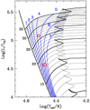 |
Fig. 9. Evolutionary tracks for solar composition stars from 10 M⊙ to 35 M⊙ computed with moderate overshooting (αover = 0.2) during core hydrogen burning (main sequence), and the subsequent helium core contraction. These and the ZAMS are represented with thick black lines. Labels on the ZAMS indicate the initial masses, given in solar units. Blue lines correspond to isochrones, labelled with their ages in million years. The observed error boxes for the components of HD 96264A are given in thick solid red lines. These are consistent with an age of ≈4.5 Myr for both components of the pair. |
One relevant problem is related to the tidal evolution of HD 96264A. We explored this possibility in order to find whether or not the eccentricity of the orbit and lack of synchronicity of the components we observed may have already undergone some appreciable evolution. In order to explore this possibility we solved the orbital evolution attributable to tides. We considered the treatment of tidal evolution given in Repetto & Nelemans (2014) which is a generalisation of those given by Hut (1981; see also Belczynski et al. 2008). We refer the interested reader to these papers for the detailed equations to be solved. The quantities to be considered are the evolution of the orbital semiaxis a (or, equivalently, the orbital period Porb), the eccentricity e, and the angular rotation ωi and inclination ii of each component with respect to the orbital plane. Here, we assumed that the evolution of the components is decoupled from the tidal evolution of the pair. This is clearly justified because the components are in a wide orbit (see Table 3). We then computed the tracks that best fit each component of HD 96264A to find the evolution of the main characteristics of the stars that determine the tidal evolution. In particular, we computed the tidal timescale, radius, and the radius of gyration k of each component as a function of time. We integrated the tidal equations for an age in excess of the one corresponding to the pair.
Quantitatively, assuming the observed values for Porb, e, and reasonable ones for ωi and ii, after 6 Myr, tides modify Porb increasing it in only ≈3% while the other quantities remain almost constant. Let us define the ratio of the stellar sizes to the orbital semiaxis as ξi ≡ Ri/a where the index indicates i = 1(2) for the more (less) massive component of the pair. Our stellar models indicate that for the more (less) massive star, ξ1 (ξ2) is in the range of 0.020–0.040 (0.015–0.02).
The equations for the rate of change of the semiaxis da/dt and the eccentricity de/dt are proportional to  . Meanwhile, the rate of change of the angular velocity of the components dωi/dt and their inclinations with respect to the plane of the orbit dii/dt are proportional to
  . Thus, with such low values for ξi it is not surprising that the tides are almost unable to modify the orbit of the pair.
The conclusion that follows is that the binary system HD 96264A was born with more or less the same orbit as that observed at present.
7. Summary and conclusions
We have determined for the first time the spectroscopic orbital parameters of HD 96264A. The few previously published RVs fit well in our orbital solution. We were able to disentangle the spectra of both components and classify the primary and secondary as O9.2 IV and B0 V(n), respectively. Our orbital solution shows that both massive stars are in a wide (P = 124.336 ± 0.008 d) and eccentric (e = 0.265 ± 0.005) binary system.
The stellar physical parameters were obtained by means of the IACOB-BROAD and IACOB-GBAT codes. We obtained projected rotational velocities of < 40 and 215 ± 11 km s−1 for the narrow and broad components, respectively, therefore differing by a factor greater than five.
The evolutionary status of the system was characterised obtaining an age of approximately 4.5 Myr. At that age, the model predicts current masses of 26.0 M⊙ and 17.9 M⊙ for each component. The spectroscopic masses obtained from IACOB-GBAT, 20.5 and 16.8 M⊙, resulted in values considerably lower than those, at least for the primary component. This is a long-standing problem in the field of massive stars known as the mass discrepancy (Herrero et al. 1992, 2002). Also, Markova et al. (2018) show that in the low-mass regime (20–30 M⊙, approximately), the discrepancy seems to be more evident, finding evolutionary masses systematically larger than the spectroscopic ones. On the other hand, comparisons with masses derived from observations of similar stars are better. Regarding radii, the agreement between both methods of calculation is even better: 10.8 R⊙ and 7.0 R⊙ versus 10.7 R⊙ and 7.1 R⊙. The comparison of these radii with determinations available in the literature for other well studied binary systems with components of similar spectral types is reasonable (see Sect.5.2.2).
It should be noted that both the evolutionary and the spectroscopic masses reproduce the mass ratio determined from the spectroscopic orbit (q = 0.660 ± 0.009) reasonably well, considering the uncertainties. The mass ratio obtained from the spectroscopic analysis is 0.82 ± 0.19 and that obtained from the evolutionary analysis is 0.69. We must reiterate here that the RVs of the broad-lined component could have uncertainties on the order of 10 km s−1 which would influence the orbital semi-amplitude and consequently the computed minimum masses. We explored orbital solutions considering the maximum errors in the RVs of the broader component, finding that the q parameter varies between 0.57 and 0.79. Of course, the best value is q = 0.66 but its error could be undervalued by the fitting code.
We also analysed the tidal evolution of the system reaching the conclusion that the current configuration is the same as at birth.
Finally, considering the youth and the wide orbit of the system, the non-synchronous nature of HD 96264A, which is either due to different rotational velocities or non-coplanar spin axes, appears to be a consequence of the formation process of the system. This fact may help to constrain the theories of binary formation.
IRAF was distributed by the National Optical Astronomy Observatories, which are operated by the Association of Universities for Research in Astronomy, Inc., under cooperative agreement with the National Science Foundation.
As a synthetic template, we used the best-fitting FASTWIND model resulting from preliminary quantitative spectroscopic analysis (see Sect. 5.2.2) of the spectrum closest to a quadrature.
Based on the algorithm of Bertiau & Grobben (1969) and implemented by F. Bareilles (available at http://ascl.net/1710.014).
Now that the binary nature of HD 96264A is known, its membership to Lodén 306 should be re-discussed. A very preliminary statistical analysis with the Gaia data of the distances to stars with proper motions similar to HD 96264A gives a statistical mode at 3.3 kpc (and a local maximum at 2.6 kpc).
Acknowledgments
We thank to the anonymous referee for helpful comments that have improved the quality of the paper. CP and RG are Visiting Astronomers of the CASLEO. CP, RG, NM, and RB are Visiting Astronomers of LCO, and RB, of La Silla/ESO. OGB is member of the Carrera del Investigador Científico of the Comisión de Investigaciones Científicas de la Provincia de Buenos Aires (CICPBA), Argentina. We thank the directors and staff of CASLEO, LCO, and La Silla/ESO for support and hospitality during our observing runs. RHB appreciates the imagination provided by “In the Observing Zone” playground. This research has made use of the SIMBAD database, operated at CDS, Strasbourg, France. This research has made use of the NASA Exoplanet Archive, which is operated by the California Institute of Technology, under contract with the National Aeronautics and Space Administration under the Exoplanet Exploration Program. This work has made use of data from the European Space Agency (ESA) mission Gaia (https://www.cosmos.esa.int/gaia), processed by the Gaia Data Processing and Analysis Consortium (DPAC, https://www.cosmos.esa.int/web/gaia/dpac/consortium). Funding for the DPAC has been provided by national institutions, in particular the institutions participating in the Gaia Multilateral Agreement.
References
- Bailer-Jones, C. A. L., Rybizki, J., Fouesneau, M., Mantelet, G., & Andrae, R. 2018, AJ, 156, 58 [NASA ADS] [CrossRef] [Google Scholar]
- Barbá, R. H., Gamen, R., Arias, J. I., et al. 2010, Rev. Mex. Astron. Astrofis. Conf. Ser., 38, 30 [Google Scholar]
- Barbá, R., Gamen, R., Arias, J. I., et al. 2014, Rev. Mex. Astron. Astrofis. Conf. Ser., 44, 148 [Google Scholar]
- Barbá, R. H., Gamen, R., Arias, J. I., & Morrell, N. I. 2017, in The Lives and Death-Throes of Massive Stars, eds. J. J. Eldridge, J. C. Bray, L. A. S. McClelland, & L. Xiao, IAU Symp., 329, 89 [Google Scholar]
- Belczynski, K., Kalogera, V., Rasio, F. A., et al. 2008, ApJS, 174, 223 [NASA ADS] [CrossRef] [Google Scholar]
- Benvenuto, O. G., & De Vito, M. A. 2003, MNRAS, 342, 50 [NASA ADS] [CrossRef] [Google Scholar]
- Benvenuto, O. G., Bersten, M. C., & Nomoto, K. 2013, ApJ, 762, 74 [NASA ADS] [CrossRef] [Google Scholar]
- Bertiau, F. C., & Grobben, J. 1969, Ric. Astron., 8, 1 [Google Scholar]
- Bosch, G., & Meza, A. 2001, Rev. Mex. Astron. Astrofis. Conf. Ser., 11, 29 [Google Scholar]
- Carraro, G., Turner, D. G., Majaess, D. J., et al. 2017, AJ, 153, 156 [CrossRef] [Google Scholar]
- Chini, R., Hoffmeister, V. H., Nasseri, A., Stahl, O., & Zinnecker, H. 2012, MNRAS, 424, 1925 [Google Scholar]
- Conti, P. S., Leep, E. M., & Lorre, J. J. 1977, ApJ, 214, 759 [NASA ADS] [CrossRef] [Google Scholar]
- Cox, A. N. 2000, Allen’s Astrophysical Quantities (Springer) [Google Scholar]
- Daflon, S., Cunha, K., de Araújo, F. X., Wolff, S., & Przybilla, N. 2007, AJ, 134, 1570 [NASA ADS] [CrossRef] [Google Scholar]
- de Mink, S. E., Langer, N., Izzard, R. G., Sana, H., & de Koter, A. 2013, ApJ, 764, 166 [NASA ADS] [CrossRef] [Google Scholar]
- Dimitrijevic, M. S., & Sahal-Brechot, S. 1990, A&AS, 82, 519 [NASA ADS] [Google Scholar]
- Duchêne, G., & Kraus, A. 2013, ARA&A, 51, 269 [Google Scholar]
- Ferrero, G. 2016, PhD Thesis, Univ. Nac. de La Plata [Google Scholar]
- García, E. V., Stassun, K. G., Pavlovski, K., et al. 2014, AJ, 148, 39 [NASA ADS] [CrossRef] [Google Scholar]
- González, J. F., & Levato, H. 2006, A&A, 448, 283 [NASA ADS] [CrossRef] [EDP Sciences] [Google Scholar]
- Herrero, A., Kudritzki, R. P., Vilchez, J. M., et al. 1992, A&A, 261, 209 [NASA ADS] [Google Scholar]
- Herrero, A., Puls, J., & Najarro, F. 2002, A&A, 396, 949 [NASA ADS] [CrossRef] [EDP Sciences] [Google Scholar]
- Holgado, G., Simón-Díaz, S., & Barbá, R. 2017, in The Lives and Death-Throes of Massive Stars, eds. J. J. Eldridge, J. C. Bray, L. A. S. McClelland, & L. Xiao, IAU Symp., 329, 407 [Google Scholar]
- Holgado, G., Simón-Díaz, S., Barbá, R. H., et al. 2018, A&A, 613, A65 [NASA ADS] [CrossRef] [EDP Sciences] [Google Scholar]
- Hut, P. 1981, A&A, 99, 126 [NASA ADS] [Google Scholar]
- Kharchenko, N. V., Piskunov, A. E., Röser, S., Schilbach, E., & Scholz, R. D. 2005, A&A, 438, 1163 [NASA ADS] [CrossRef] [EDP Sciences] [MathSciNet] [Google Scholar]
- Lindroos, K. P. 1985, A&AS, 60, 183 [NASA ADS] [Google Scholar]
- Lodén, L. O. 1980, A&AS, 41, 173 [Google Scholar]
- Lorenz, R., Mayer, P., & Drechsel, H. 1998, A&A, 332, 909 [NASA ADS] [Google Scholar]
- Maíz Apellániz, J., & Barbá, R. H. 2018, A&A, 613, A9 [NASA ADS] [CrossRef] [EDP Sciences] [Google Scholar]
- Markova, N., Puls, J., & Langer, N. 2018, A&A, 613, A12 [NASA ADS] [CrossRef] [EDP Sciences] [Google Scholar]
- Martin, N. 1967, J. Obs., 50, 203 [Google Scholar]
- Martins, F., Schaerer, D., & Hillier, D. J. 2005, A&A, 436, 1049 [NASA ADS] [CrossRef] [EDP Sciences] [Google Scholar]
- Mason, B. D., Gies, D. R., Hartkopf, W. I., et al. 1998, AJ, 115, 821 [NASA ADS] [CrossRef] [Google Scholar]
- Mason, B. D., Wycoff, G. L., Hartkopf, W. I., Douglass, G. G., & Worley, C. E. 2001, AJ, 122, 3466 [Google Scholar]
- Mayer, P., Harmanec, P., Nesslinger, S., et al. 2008, A&A, 481, 183 [NASA ADS] [CrossRef] [EDP Sciences] [Google Scholar]
- Nieva, M.-F., & Przybilla, N. 2014, A&A, 566, A7 [NASA ADS] [CrossRef] [EDP Sciences] [Google Scholar]
- Petrovic, J., Langer, N., & van der Hucht, K. A. 2005, A&A, 435, 1013 [NASA ADS] [CrossRef] [EDP Sciences] [Google Scholar]
- Puls, J., Urbaneja, M. A., Venero, R., et al. 2005, A&A, 435, 669 [NASA ADS] [CrossRef] [EDP Sciences] [Google Scholar]
- Putkuri, C., Gamen, R., Morrell, N. I., et al. 2018, A&A, 618, A174 [CrossRef] [EDP Sciences] [Google Scholar]
- Repetto, S., & Nelemans, G. 2014, MNRAS, 444, 542 [NASA ADS] [CrossRef] [Google Scholar]
- Repolust, T., Puls, J., & Herrero, A. 2004, A&A, 415, 349 [NASA ADS] [CrossRef] [EDP Sciences] [Google Scholar]
- Rivero González, J. G., Puls, J., Massey, P., & Najarro, F. 2012, A&A, 543, A95 [NASA ADS] [CrossRef] [EDP Sciences] [Google Scholar]
- Ryans, R. S. I., Dufton, P. L., Rolleston, W. R. J., et al. 2002, MNRAS, 336, 577 [NASA ADS] [CrossRef] [Google Scholar]
- Sabín-Sanjulián, C., Simón-Díaz, S., Herrero, A., et al. 2014, A&A, 564, A39 [NASA ADS] [CrossRef] [EDP Sciences] [Google Scholar]
- Sana, H., & Evans, C. J. 2011, in Active OB Stars: Structure, Evolution, Mass Loss, and Critical Limits, eds. C. Neiner, G. Wade, G. Meynet, & G. Peters, IAU Symp., 272, 474 [Google Scholar]
- Sana, H., de Mink, S. E., de Koter, A., et al. 2012, Science, 337, 444 [Google Scholar]
- Sana, H. 2017, in The Lives and Death-Throes of Massive Stars, eds. J. J. Eldridge, J. C. Bray, L. A. S. McClelland, & L. Xiao, IAU Symp., 329, 110 [Google Scholar]
- Santolaya-Rey, A. E., Puls, J., & Herrero, A. 1997, A&A, 323, 488 [NASA ADS] [Google Scholar]
- Scargle, J. D. 1982, ApJ, 263, 835 [Google Scholar]
- Simón-Díaz, S., & Herrero, A. 2007, A&A, 468, 1063 [NASA ADS] [CrossRef] [EDP Sciences] [Google Scholar]
- Simón-Díaz, S., & Herrero, A. 2014, A&A, 562, A135 [NASA ADS] [CrossRef] [EDP Sciences] [Google Scholar]
- Simón-Díaz, S., Castro, N., Herrero, A., et al. 2011, J. Phys. Conf. Ser., 328, 012021 [NASA ADS] [CrossRef] [Google Scholar]
- Sota, A., Maíz Apellániz, J., Walborn, N. R., et al. 2011, ApJS, 193, 24 [Google Scholar]
- Sota, A., Maíz Apellániz, J., Morrell, N. I., et al. 2014, ApJS, 211, 10 [Google Scholar]
- Thackeray, A. D., Tritton, S. B., & Walker, E. N. 1973, MmRAS, 77, 199 [NASA ADS] [Google Scholar]
- Tüysüz, M., Soydugan, F., Bilir, S., et al. 2014, New Astron., 28, 44 [Google Scholar]
- Wellstein, S., Langer, N., & Braun, H. 2001, A&A, 369, 939 [NASA ADS] [CrossRef] [EDP Sciences] [Google Scholar]
- Zhang, Y., Tan, J. C., Tanaka, K. E. I., et al. 2019, Nat. Astron., 224, [Google Scholar]
All Tables
Radial velocity measurements (km s−1) of both components in the HD 96264A system.
Orbital parameters of the HD 96264A system derived from the radial velocity curve.
Parameters obtained from the spectroscopic analysis of both components of HD 96264A.
All Figures
|
Fig. 1. Section of the LCO spectra of HD 96264A obtained near both quadratures. The upper box on the right side of the figure shows LCO and ESO spectra in the region of He Iλ5876 obtained at different orbital phases in order to illustrate the observed variation in the line profile. The phases of the different observations, according to the ephemerides of Table 2, are indicated above the correspondent spectrum. |
| In the text | |
|
Fig. 2. Periodograms of the primary RVs obtained with the NASA Exoplanet Archive Periodogram Service. In black, the OWN Survey dataset; in violet, the OWN Survey dataset plus five RVs gathered from the literature. |
| In the text | |
|
Fig. 3. RV curves of the primary (blue) and secondary (red) components of the binary system HD 96264A calculated with the parameters of the orbital solution shown in Table 3 along with the observations. Errors on primary RVs are smaller than the symbol sizes. Filled circles represent LCO and La Silla data, and open circles are used for CASLEO. Yellow circles represent the previously published RVs. The O-C for the primary (blue) and secondary (red) are depicted in the bottom panel. |
| In the text | |
|
Fig. 4. Normalised disentangled spectra of the primary (shifted upwards by 0.42 continuum units) and secondary components of HD 96264A system. Relevant features for spectral classification are indicated. Some artefacts on the spectra, mostly seen in the wings of the hydrogen lines, are originated in the disentangling process. |
| In the text | |
|
Fig. 5. Graphical output of the IACOB-BROAD tool for both stellar components of HD 96264A. The left upper panel shows the line profile of O IIIλ5592 of the primary component and the right upper panel shows its Fourier transform. The bottom panels show similar plots for the He Iλ5015 line of the secondary component. Four fits are presented in each case: v sin i(FT) in red, (v sin i, vmac) (GOF) in blue, (v sin i, vmac = 0.0) (GOF) in green, and (v sin i = FT, vmac) (GOF) in violet. |
| In the text | |
|
Fig. 6. Template of the narrow component of HD 96264A overplotted on the best fit from the IACOB-GBAT grid (solid black lines). The v sin i and vmac employed were those previously determined. The colours correspond to the spectral regions employed in the analysis (red) and discarded (sky blue). |
| In the text | |
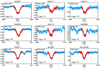 |
Fig. 7. Same as Fig. 6 but for the template of the broad component of HD 96264A. |
| In the text | |
|
Fig. 8. Composite FEROS spectrum of HD 96264A (in grey) compared to a combined synthetic model (in sky blue) resulting from the best fitting FASTWIND models to each stellar component (Teff = 33 kK, log g = 3.70 dex and log Q = −12.7 for component A; Teff = 30 kK, log g = 3.90 dex and log Q = −12.7 for component B). Both individual models were diluted and added in order to obtain the composed model. All FASTWIND models in this figure have YHe = 0.09 and β = 0.8. |
| In the text | |
|
Fig. 9. Evolutionary tracks for solar composition stars from 10 M⊙ to 35 M⊙ computed with moderate overshooting (αover = 0.2) during core hydrogen burning (main sequence), and the subsequent helium core contraction. These and the ZAMS are represented with thick black lines. Labels on the ZAMS indicate the initial masses, given in solar units. Blue lines correspond to isochrones, labelled with their ages in million years. The observed error boxes for the components of HD 96264A are given in thick solid red lines. These are consistent with an age of ≈4.5 Myr for both components of the pair. |
| In the text | |
Current usage metrics show cumulative count of Article Views (full-text article views including HTML views, PDF and ePub downloads, according to the available data) and Abstracts Views on Vision4Press platform.
Data correspond to usage on the plateform after 2015. The current usage metrics is available 48-96 hours after online publication and is updated daily on week days.
Initial download of the metrics may take a while.