| Issue |
A&A
Volume 650, June 2021
|
|
|---|---|---|
| Article Number | A58 | |
| Number of page(s) | 23 | |
| Section | Stellar structure and evolution | |
| DOI | https://doi.org/10.1051/0004-6361/202039543 | |
| Published online | 07 June 2021 | |
Constraining stellar evolution theory with asteroseismology of γ Doradus stars using deep learning
Stellar masses, ages, and core-boundary mixing
1
Institute of Astronomy, KU Leuven, Celestijnenlaan 200D, 3001 Leuven, Belgium
e-mail: This email address is being protected from spambots. You need JavaScript enabled to view it.
2
Department of Astrophysics, IMAPP, Radboud University Nijmegen, PO Box 9010, 6500 GL Nijmegen, The Netherlands
3
Max Planck Institute for Astronomy, Koenigstuhl 17, 69117 Heidelberg, Germany
Received:
28
September
2020
Accepted:
19
March
2021
Abstract
Context. The efficiency of the transport of angular momentum and chemical elements inside intermediate-mass stars lacks proper calibration, thereby introducing uncertainties on a star’s evolutionary pathway. Improvements require better estimation of stellar masses, evolutionary stages, and internal mixing properties.
Aims. Our aim was to develop a neural network approach for asteroseismic modelling, and test its capacity to provide stellar masses, ages, and overshooting parameter for a sample of 37 γ Doradus stars; these parameters were previously determined from their effective temperature, surface gravity, near-core rotation frequency, and buoyancy travel time Π0. Here our goal is to perform the parameter estimation from modelling of individual periods measured for dipole modes with consecutive radial order rather than from Π0. We assess whether fitting these individual mode periods increases the capacity of the parameter estimation.
Methods. We trained neural networks to predict theoretical pulsation periods of high-order gravity modes (n ∈ [15, 91]), and to predict the luminosity, effective temperature, and surface gravity for a given mass, age, overshooting parameter, diffusive envelope mixing, metallicity, and near-core rotation frequency. We applied our neural networks for Computing Pulsation Periods and Photospheric Observables (C-3PO) to our sample and compute grids of stellar pulsation models for the estimated parameters.
Results. We present the near-core rotation rates (from the literature) as a function of the inferred stellar age and critical rotation rate. We assessed the rotation rates of the sample near the start of the main sequence assuming rigid rotation. Furthermore, we measured the extent of the core overshoot region and find no correlation with mass, age, or rotation. Finally, for one star in our sample, KIC 12066947, we find indications of mode coupling in the period spacing pattern which we cannot reproduce with mode trapping.
Conclusions. The neural network approach developed in this study allows the derivation of stellar properties dominant for stellar evolution, such as mass, age, and extent of core-boundary mixing. It also opens a path for future estimation of mixing profiles throughout the radiative envelope, with the aim of inferring these profiles for large samples of γ Doradus stars.
Key words: asteroseismology / stars: evolution / stars: oscillations / stars: rotation / stars: interiors
© ESO 2021
1. Introduction
Accurate predictions of a star’s evolutionary path depend on the accuracy of the description of transport of angular momentum (AM, e.g. Maeder 2009; Aerts et al. 2019) and chemical elements (e.g. Salaris & Cassisi 2017). The transport mechanisms are still poorly understood, thereby introducing uncertainties in state-of-the-art stellar structure and evolution models. These uncertainties already occur during the core-hydrogen burning stage, and hence propagate into models of more evolved stars as well. Asteroseismology, the study of stellar oscillations, in low- to intermediate-mass stars (M⋆ ≲ 3.3 M⊙) constitutes a powerful tool to measure surface and near-core rotation rates across various evolutionary phases: main sequence (MS; Kurtz et al. 2014; Saio et al. 2015; Van Reeth et al. 2016, 2018; Christophe et al. 2018; Ouazzani et al. 2017); subgiants and red giants (Beck et al. 2012; Mosser et al. 2012; Gehan et al. 2018); and white dwarfs (Hermes et al. 2017). The empirically derived rotation rates require the transport of AM to be one to two orders of magnitude more efficient than what is currently predicted by theory (e.g. Cantiello et al. 2014; Fuller et al. 2014, 2019; Eggenberger et al. 2017, 2019a,b; Tayar & Pinsonneault 2018; den Hartogh et al. 2019, 2020). It has been suggested by Eggenberger et al. (2017) that the efficiency of AM transport increases with increasing mass.
Aerts et al. (2019, their Fig. 4) present an overview of measured core rotation rates versus the surface gravity (log g) in the literature for stars with M⋆ ∈ [0.72, 7.9] M⊙. While the different evolutionary stages can be distinguished based on log g, the typical uncertainty is too large to infer any correlations between the rotation rate and the stellar age (Aerts et al. 2017). Instead of using log g as an age proxy, Ouazzani et al. (2019) used the reduced asymptotic period spacing Π0, which represents the buoyancy travel time throughout the star, as derived for a sample of γ Doradus (γ Dor) stars. Such stars are of spectral types from late A to early F (1.4 M⊙ ≲ M⋆ ≲ 1.9 M⊙) and show gravity (g) modes excited via a convective flux blocking mechanism (e.g. Guzik et al. 2000; Dupret et al. 2005), although the κ mechanism also plays a role for the hotter members of the class (Xiong et al. 2016).
In a chemically homogeneous non-rotating non-magnetic star, the periods of g modes (with the same spherical degree ℓ and azimuthal order m, but consecutive radial order n) are equally spaced in period in the asymptotic regime (n ≫ ℓ), namely by  . It is therefore customary to present the oscillations in a period spacing diagram, where the spacing ΔP = Pn + 1 − Pn of each individual mode with radial order n is plotted as a function of its period Pn. The advent of the Kepler (Borucki et al. 2010) and TESS (Ricker et al. 2015) missions have led to numerous detections of such period spacing patterns in γ Dor stars (Kurtz et al. 2014; Saio et al. 2015, 2018; Van Reeth et al. 2015; Keen et al. 2015; Li et al. 2019, 2020; Antoci et al. 2019). A first attempt at estimating stellar masses and ages of a sample of 37 γ Dor stars was done by Mombarg et al. (2019) using Π0, Teff, and log g assembled in Van Reeth et al. (2015, 2016) as input for the modelling. Their results show that faster rotating stars tend to be in the early phases of the MS, and there was no correlation between age and the detection of Rossby modes. In this paper our aim is to refine their work by fitting the measured periods for each of the individual dipole modes with consecutive radial order instead of just Π0 as asteroseismic observable.
In addition to probing stellar rotation rates, asteroseismology also allows the scrutiny of a star’s internal chemical mixing profile (e.g. Pedersen et al. 2018, 2021; Michielsen et al. 2019). During the core-hydrogen burning phase, a chemical gradient is introduced in the near-core region as the mean molecular weight inside the core increases.
The presence of a chemical gradient causes mode trapping, which translates into characteristic dips in the period spacing pattern (Miglio et al. 2008). However, mixing occurs in the core boundary layers, due to effects such as core overshooting and a variety of phenomena occurring at the bottom of the envelope. In addition, mixing throughout the radiative envelope occurs, for example as a result of shear instabilities (Maeder 2009) or internal gravity waves (e.g. Rogers & McElwaine 2017). Such forms of mixing alter the chemical gradient, making it possible to probe the efficiency of the mixing throughout the stellar envelope and infer properties of the mixing profile provided that modes with suitable probing power can be detected and identified (Aerts 2021). This has been achieved for a sample of B-type g-mode pulsators, revealing a wide range of mixing levels, from ∼10 to ∼106 cm2 s−1 (Pedersen et al. 2021). For γ Dor stars our understanding of mixing in the envelope is less advanced because their levels of mixing at the deep bottom of the envelope, at the interface with the core overshoot zone, were found to be much lower (Van Reeth et al. 2016; Mombarg et al. 2019).
In this paper we take the first steps towards developing a new modelling approach based on deep learning, with the future aim of estimating the mixing profile throughout the radiative envelope of γ Dor stars. In this initial study we only treat the mixing in the near-core boundary layer, while fixing the one in the outer envelope. We do this because we first aim to assess the precision estimation of the global stellar parameters, such as the mass, metallicity, age, and convective core overshooting for an exponential overshooting prescription, by relying on the individual mode period spacings rather than on just Π0. In order to test the capacity of our new deep learning method we re-model the measured period spacing patterns of the 37 γ Dor stars from the sample of Van Reeth et al. (2015) and derive masses, ages, and near-core mixing efficiencies. These are then compared to those obtained earlier by Mombarg et al. (2019). If we achieve a better modelling strategy based on our initial deep learning approach, then future applications in a much higher-dimensional parameter space become possible, which would allow the additional estimation of the envelope mixing profiles responsible for the observed morphologies of the period spacing patterns in terms of isolated or recurring dips, as observed by Van Reeth et al. (2015), Li et al. (2019, 2020).
2. Deep learning
One of the biggest challenges in asteroseismic modelling of period spacing patterns is that it requires a parameter search in high-dimensional space. The most important parameters are the stellar mass (M⋆), the initial metallicity Z, and the hydrogen mass fraction in the convective core (Xc, a proxy for the stellar age). In addition, the chemical mixing profile is typically split in two parts: the convective core overshooting (dark regions in Fig. 1) and the mixing efficiency in the radiative envelope (labelled D0 in Fig. 1). Given that the physical mechanisms at stake are still unknown, both the overshoot and envelope mixing profile are parametrised by a function dependent on the local radius r, where the exact functional description in real stars is still a matter of debate (e.g. Aerts 2021, for a general discussion and example profiles). Mombarg et al. (2019) showed that diffusive exponentially decaying core overshooting cannot be distinguished from convective penetration in their modelling based on Π0. As our main aim here is to evaluate our new deep learning modelling method (in terms of its capacity to estimate the global parameters) and not to investigate the detailed morphology of the period spacing patterns, we rely on an exponentially decaying diffusive core overshooting prescription. Our focus thus lies on the parameter estimation delivered by the individual period spacing values coupled to a neural network. The diffusive overshooting is expressed as a dimensionless parameter fov times the pressure scale height (Freytag et al. 1996)
 (1)
(1)
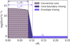 |
Fig. 1. Chemical mixing profile showing the different mixing zones in a model for an intermediate-mass star. The ordinate shows the local efficiency of chemical (diffusive) mixing. The thin outer convection zone is not shown in the plot. The radii of the convective core boundary (rcc) and overshoot zone (rov) are also indicated. Mixing inside the convective regions is based on MLT and occurs instantaneously. The red dashed line slightly to the left of rcc/R⋆ indicates the starting point of the overshoot zone (r0 in Eq. (1)). |
where rcc and HP are the distance from the stellar centre to the (Schwarzschild) core boundary and pressure scale height, respectively. For numerical purposes the mixing efficiency at the stitching point between convective mixing in the core and the core overshoot mixing is evaluated at rcc − f0HP(rcc), for which we set f0 = 0.005. As said, we do not focus on the shape of the mixing profile in the outer radiative envelope in this first application of the neural network. Hence, we assume a constant mixing efficiency throughout the radiative zone for simplicity.
Aside from these most important parameters for determining the stellar structure and evolution (SSE) models, M⋆, Z, Xc, and fov, we introduce the internal rotation frequency frot at the level of the pulsation computations. Hence, asteroseismic modelling of stars with a convective core is in general a +6D problem (Aerts et al. 2018; Aerts 2021). This modelling scheme rapidly becomes computationally expensive with the option to also assess mixing profiles via free parameters and for application to large γ Dor sample sizes such as the one provided by Li et al. (2020). To deal with such types of future applications, grids of stellar or pulsation models can be approximated and replaced by statistical models (Mombarg et al. 2019; Pedersen et al. 2021) or neural networks (this work). The latter method has been applied to non-rotating pulsation models for a benchmark sample of pulsating B-type stars by Hendriks & Aerts (2019), reaching an accuracy of ∼10% on the pulsation frequencies predicted by deep learning models, compared to those from the pulsation models. The observed values for Z and frot show that the stars in our sample cover a large range. Furthermore, the γ Dor instability strip is narrow compared to those of other pulsators. As such, properly covering the most important stellar parameters with an equally spaced linear grid set-up, as is commonly done in asteroseismic modelling, would require a very large number of equilibrium models. We want to circumvent this by replacing the need of such extensive model grids by a neural network (NN). This study serves as an initial proof-of-concept study of the application of deep learning to asteroseismic modelling of g-mode pulsators, with the idea that future studies may rely on a larger set of grids with different input physics.
2.1. Predicting pulsation periods
For this work we trained a NN to predict g-mode periods of theoretical pulsation models for given values of M⋆, Xc, Z, fov, D0, and frot. We chose this approach instead of using the asteroseismic data as input and the stellar parameters as output (e.g. Hon et al. 2020) because it allows more flexibility in the number of free parameters, as we can fix some of these parameters without having to retrain the NN. We kept this outlook in mind for future applications based on more complex envelope mixing profiles. In this initial study we computed a grid of stellar equilibrium models for the parameter ranges listed in Table 1 based on the ranges used in Mombarg et al. (2019). We based our range of fov on the typical values found by Claret & Torres (2017) for the appropriate mass regime. The parameter space was sampled linearly and quasi-randomly from a Sobol sequence, following Bellinger et al. (2016). This way we obtained a high sampling density for each parameter, whilst also allowing the parameters to vary independently. The stellar equilibrium models were computed with the SSE code MESA (r11701) (Paxton et al. 2011, 2013, 2015, 2018, 2019) for the computations of the stellar equilibrium models, using the same input physics as the models without atomic diffusion described in Mombarg et al. (2020). The stars in our sample are assumed to have a chemical mixture similar to the Sun, that is, we take the solar abundances from Asplund et al. (2009), and scale them according to the metallicity Z. The helium mass fraction of the models are set according to the enrichment rate found by Verma et al. (2019) and the initial hydrogen mass fraction is set by Xini = 1 − Yini − Z = 0.756 − 2.226Z with the 2H/1H and 3He/4He isotope ratios set to the values measured by Asplund et al. (2009).
Extent of the grid of stellar models used to train the C-3PO neural network.
From the stellar equilibrium models, the theoretically predicted pulsations are computed with the pulsation code GYRE (v5.2; Townsend & Teitler 2013; Townsend et al. 2018), using the adiabatic framework and treating the Coriolis acceleration non-perturbatively. The equations of motion are decoupled in the angular and radial components by neglecting the latitudinal component of the rotation vector (traditional approximation of rotation, TAR; Eckart 1960; Townsend 2003). Analyses of large samples of γ Dor stars by Van Reeth et al. (2016) and Li et al. (2020) reveal that the prograde dipole mode (ℓ = 1, m = 1) is by far the most observed mode geometry. Hence, for each stellar equilibrium model we computed the predicted pulsation frequencies for (ℓ,m) = (1, 1) modes and radial orders n ∈ [15, 91] (thus ΔPn for n ∈ [15, 90]), using the pulsation code GYRE (Townsend 2003; Townsend & Teitler 2013). The range of radial orders is based on the distribution found by Li et al. (2020), taking the most ubiquitous ones. Again, we quasi-randomly sampled Xc and frot within the ranges listed in Table 1. The rotation frequency range is based on the minimum and maximum observed values in the sample of Van Reeth et al. (2016). The total output data set contains 38915 pulsation models, of which 70% are used for training and 30% for validation.
Neural networks are powerful numerical methods suitable for treating multi-dimensional and complex regression problems (see Bishop 1995; Glorot et al. 2011, for an introduction and general overview on deep learning). We constructed a dense NN comprising five layers, using the KERAS package for Python (with Tensorflow 1.14.0), for which the schematic overview of the NN is shown in Fig. 2. A rectified linear unit (ReLU) was used as the activation function for the neurons of the first four layers, and a linear activation function for the output layer, including a bias term for both activation functions. We tested several of the most commonly used activation functions (ReLU, sigmoid, tanh), for which we found that the ReLU activation functions yielded the best performance for our NN. The output of the NN are the predicted periods of radials orders n ∈ [15, 91].
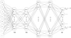 |
Fig. 2. Schematic overview of the configuration of the dense neural network trained to predict the periods of the (ℓ, m) = (1,1) modes for a given θ = (M⋆, Xc, Z, fov, D0, frot, M⋆ ⋅ Xc, M⋆ ⋅ Z). The values of the input parameters are transformed following Eq. (2). |
Similarly constructing statistical models as a means to represent reality, adding non-linear combinations of the input parameters can increase the performance of a NN. Inspired by the regressions performed in Mombarg et al. (2019), we found the performance of our NN to be enhanced by adding two product terms of the most correlated parameters, the mass and age, and mass and metallicity, to the input vector θ = (M⋆, Xc, Z, fov, D0, frot, M⋆ ⋅ Xc, M⋆ ⋅ Z). Each component of θ is normalised as
 (2)
(2)
where i is the parameter index and j the model index. The technique of ‘early stopping’ is applied to prevent the loss from increasing again after several epochs; that is, the training is terminated when the validation loss has not decreased during three consecutive epochs. The weights are then restored to the configuration for which the validation loss was the lowest.
The problem of overfitting is common when training a NN; that is, the NN achieves a high precision on the training set while it fails to generalise the correlations, and thus underperforms on the validation set. To remedy overfitting a penalty term  is added to the loss function, where wj are the synaptic weights and λ the control parameter, which we set to 0.01. This technique penalises large weights and is commonly referred to as L2 or ridge regularisation (see Bishop 1995, Chap. 9.2). As a loss function, the mean squared error is used. The final configuration of the weights is somewhat dependent on the initial weights, which introduces noise in the predictions. To remedy this we train six NNs with different initial weights and average their predictions; this technique is often referred to as ensemble learning.
The so-called learning curve is a common diagnostic to assess whether a NN is able to make robust predictions. This curve shows the loss (which includes the L2 regularisation term) as a function of epoch. In the top panel of Fig. 3 we show the learning curves for all NNs trained to predict the pulsation periods. Ideally, a NN should obtain roughly the same loss on the training and validation set, which is indeed the case here. When ensemble learning is applied, a mean absolute error of 0.0024 d (207 s) on the pulsation periods is obtained over all models used to train and validate the NN. Typical observed spacings between periods of consecutive radial order vary from several hundreds to several thousands of seconds. It is more instructive to compare the accuracy of the NN with typical spacings rather than observational uncertainties as the accuracy of the state-of-the-art pulsation models is typically orders of magnitude worse than the uncertainties on the measured periods from Kepler light curves (e.g. Buysschaert et al. 2018; Mombarg et al. 2020).
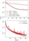 |
Fig. 3. Loss (mean squared error + L2 regularisation term) as a function of epoch. The NNs training on the pulsation models (bottom panel) reached an optimal solution within the maximum number of epochs. In all cases a similar loss is obtained for the training and validation sets, indicating the NNs were able to generalise the synaptic weights. |
2.2. Lifting degeneracies
The modelling of mode periods or period spacing patterns is prone the degeneracies, mainly between mass and age, and mass and metallicity (e.g. Moravveji et al. 2015; Mombarg et al. 2019, 2020). We apply the same methodology as Mombarg et al. (2020), where the best model is selected from models that are compatible with the effective temperature (Teff) and surface gravity (log g), measured from spectroscopy. In addition to these two parameters, the luminosity (log(L/L⊙)) derived from the Gaia DR2 distances (D) measured by Bailer-Jones et al. (2018) is used:
![Mathematical equation: $$ \begin{aligned} \log L/{L_\odot } = -0.4\left(M_{V} - V_\odot - 31.572 + [\mathrm{BC}_V - \mathrm{BC}_{V,\odot }]\right). \end{aligned} $$](/articles/aa/full_html/2021/06/aa39543-20/aa39543-20-eq5.gif) (3)
(3)
Here MV = mV − 5log(D/10 pc)−3.3E(B − V), V⊙ = −26.76, and BCV, ⊙ = −0.080. Bolometric corrections (BCV) are computed following Torres (2010), and reddening corrections E(B − V) are taken from the Bayerstar2019 extinction map (Green et al. 2018). From the extinction, the correction to the visual magnitude is calculated using AV = 3.3E(B − V). Figure 4 shows the position of all stars in our sample in a Hertzsprung-Russell diagram (see Table A.1).
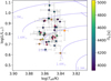 |
Fig. 4. Positions in the Hertzsprung-Russel diagram of all stars in our sample. The values of Teff and Π0 are taken from Van Reeth et al. (2016). The evolution tracks shown are for Z = 0.014 and fov = 0.0175. For the stars marked with red circles no reliable extinction estimate could be made because they are too close to the Sun, and therefore their interstellar extinction values are close to zero. |
In addition to the mode periods, we trained two NNs to predict (Teff, log g) and log L, using the same configuration as the network shown in Fig. 2. To train these NNs, we use all the time steps (on the MS) computed by MESA as opposed to using only the time step for which pulsation models were computed, which means that the training set comprises 423691 vectors and the validation set comprises 141231 vectors. In Fig. 5 we compare the predictions of the NNs of these photospheric observables to MESA evolutionary tracks. We obtain mean absolute errors of  , and
, and  dex on the complete data set (training plus validation). The models shown in this figure were not included in the training or validation set. There is no exact method to find the optimal configuration of a NN. We started from a network configuration similar to that presented in Hendriks & Aerts (2019), and experimented with different numbers of hidden layers, and the number of neurons per layer, by means of trial and error. Table 2 summarises the ensemble of all the networks for Computing Pulsation Periods and Photospheric Observables (C-3PO).
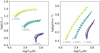 |
Fig. 5. Comparison between the predictions of C-3PO (dots) and the MESA benchmark evolution tracks (solid lines) for Z = 0.012 and Z = 0.023. The predictions are sampled from Xc = 0.70 to 0.05 with a step size of 0.05. |
Summary of the network configuration of C-3PO.
3. Asteroseismic modelling
Until recently, g-mode modelling of single γ Dor stars relied on (Π0, Teff, log g) as input (Mombarg et al. 2019). In the work by Mombarg et al. (2020), Π0 is replaced with the individual mode periods as asteroseismic input for the modelling of two slowly rotating γ Dor stars. Furthermore, these authors investigated whether Teff and log g should be added to the fit or used a posteriori to select models that are consistent within nσ compared to the observations. As typically tens of excited modes of consecutive radial order are observed in a single star, the spectroscopic observables have little relative weight in the merit function. Therefore, we opted to use the log Teff and log g to select the best-fitting model from a subset of models which are within the 2σ uncertainty ranges of these photospheric observables. Aerts et al. (2018) introduced the Mahalanobis distance (MD) as a merit function in asteroseismic modelling to account for the correlated nature of the observed periods and for the theoretical uncertainty of the modes. The MD takes the (co)variances of the input parameters into account such that the contours of equal MD are aligned with the principal components, whereas for the χ2 merit function contours of equal χ2 are aligned with the base vectors (free parameters). For a given vector Y(th), containing the periods of the identified radial orders, and a vector Y(obs) containing the observed periods, the MD is defined as
 (4)
(4)
The matrix V is the (co)variance matrix and Σ is a diagonal matrix, constructed from the uncertainties on the predicted mode periods by the NN. These can be treated as aleatoric, as the residuals on the training and validation set follow a normal distribution (see Appendix C). Therefore, each uncertainty  , with n the radial order, is taken to be the standard deviation of the residuals over the complete grid of pulsation models. The uncertainties of the predictions are typically two orders of magnitude larger than those from the observations.
The matching between the observed radial orders to those from a model is non-trivial. Observed period spacing patterns of γ Dor stars do not always form a single sequence of consecutive radial orders, but may be interrupted by missing modes. Therefore, the radial order matching in this paper is performed as follows:
1. Start with the longest observed continuous sequence of M periods and assign the shortest period  to the best-matching period
  as the shortest period has the smallest relative uncertainty;
2. Assign periods  to the consecutive radial orders in the model;
3. Repeat step 1 for the second longest sequence, and so on. When a radial order is selected that has already been assigned to an observed period in one of the longer sequences, omit the model.
In this way we account for the possibility of having multiple sequences of consecutive radial orders with missing modes between these sequences. The construction of V can be done in two ways. In method 1, for each evaluated model j, each of the observed periods  is matched with a period
  corresponding to a radial order that may vary for different models. Matrix V is given by
 (5)
(5)
where q is the number of evaluated models, and
 (6)
(6)
In method 2 we take  to contain the periods of all the radial orders predicted by the NN, that is, n ∈ [15, 91], and construct V, thereby yielding a matrix with dimensions 77 × 77. Consecutively, for each model with radial order identifications nmin, …, nmax corresponding to the N observed mode periods, we remove the rows and columns of V belonging to the radial orders that were not identified in model j, yielding an N × N matrix, V′j.
In this paper, we used method 2 to compute the MD, such that the (co)variances do not depend on the radial order identification. This is the case for method 1 because the lowest period is matched first and the consecutive periods are then matched to the consecutive radial orders of the model. Hence, when the observed Π0 does not match the Π0 of the model, the discrepancy between the model and observations is larger for higher radial orders. Therefore, the variance across the grid will also be larger for these radial orders, and by extension will be given a smaller weight. The maximum likelihood estimate (MLE) for our method is not equivalent to minimising the merit function, as is the case for χ2. Instead, the likelihood of the observed data D, given parameters θ = (θ1, θ2, θ3), is given by
 (7)
(7)
where k = 3 is the number of free parameters. According to Bayes’ theorem, the probability of component θk being within interval ![Mathematical equation: $ [\theta_a^k, \theta_b^k] $](/articles/aa/full_html/2021/06/aa39543-20/aa39543-20-eq19.gif) is given by
is given by
 (8)
(8)
The sum over index i is taken over the q models with the highest likelihood such that  , where the sum over index j is taken over all of the models that are consistent with the observed photospheric observables.
The modelling of g modes in γ Dor stars is a high-dimensional, degenerate problem. Optimising all six parameters at once will lead to noisy solution spaces, making uncertainty determination unwieldy. However, some parameters are more dominant than others, and thus we first focus on the parameters that have the largest influence on the mode periods. Since the metallicity and near-core rotation rate have already been determined by Van Reeth et al. (2016), we fix these two parameters to the measured values. The influence of fov, and specifically D0, on the period spacings are mostly seen in the mode trapping. In this work our aim is not to precisely model the trapped modes, but rather get an accurate fit to the global pattern of all observed modes. Accurately modelling trapped modes adds additional dimensionality to the problem in the form of structured (non-constant) mixing profiles (Pedersen et al. 2021), which we do not consider here. For each star in our sample a best-fitting model is found as follows:
1. Randomly sample 5000 models in (M⋆, Xc, fov) with C-3PO, where Z and frot are fixed to the measured values, and D0 = 1 cm2 s−1;
2. If some observed periods cannot be matched in 90% of the models (because the radial order is outside the range of NN) remove either the shortest or the longest period depending on which one is outside the range. Repeat until a model can be matched;
3. From these 5000 models get the minimum and maximum values of M⋆ and Xc such that the predicted log(L/L⊙), log Teff, and log g are consistent within 2σ of the respective uncertainties;
4. Randomly sample 15 000 models, but now within the mass and Xc ranges obtained in the previous step. The solution and uncertainties are computed according to Eqs. (7) and (8);
5. Since the exact periods of trapped modes are difficult for a NN to predict, we optimise the overshoot parameter with GYRE models once we have a good estimate of (M⋆, Xc, fov) from the previous steps. We compute GYRE models for fov ∈ [0.005, 0.010, 0, 015, 0.020, 0.025, 0.030, 0.035] for the MLEs for M⋆ and Xc and for the upper and lower limits of these two parameters (63 models per star in total). Models rotating faster than the critical Roche frequency,  , are not taken into account.
In the last step a χ2 merit function is used instead of the MD as scanning such a small parameter range results in (co)variance matrices with very high condition numbers. The uncertainties on fov are determined by
 (9)
(9)
For stars where an additional mode geometry has been observed, the corresponding pulsation models are also computed and fitted simultaneously with the prograde dipole modes in Step 5.
3.1. Theoretical benchmark
First, we demonstrate the capabilities of C-3PO by applying the NN to a set of benchmark models (1.35 M⊙, 1.65 M⊙, 1.95 M⊙) which were not included in the training and validation set. We use radial orders n ∈ [20, 60], and the photospheric observables from the MESA model as input, where we assume the following uncertainties: σlog L/L⊙ = 0.05 dex, σlog Teff = 0.015 dex, and σlog g = 0.6 dex. The metallicity and rotation frequency are fixed to the values of the models in the fit since these are also known for the observations. Two examples are shown in Fig. 6, for a young star and an old star. The accuracy of the NN is lower for patterns with clear mode trapping, yet in both cases the periods are still predicted with enough accuracy such that, with the inclusion of the photospheric observables, M⋆ and Xc can be recovered. In Fig. 7, we show the mass and Xc values of all the inputs models, and the obtained estimates from C-3PO. On average the input mass, Xc, and fov are recovered within 2%, 15%, and 16%, respectively. It should also be noted that, as mentioned before, degeneracies exist between young lower-mass stars and old higher-mass stars. Thus, even if the NN were able to perfectly predict the pulsation periods, exactly recovering a (perturbed) input model would still be impossible (see middle panels of Fig. 6).
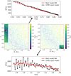 |
Fig. 6. Examples of the recovered mass and Xc of two benchmark models (white stars: input; red stars: best model predicted by NN). Although the period spacings of trapped modes are more difficult to predict (bottom panel), the inclusion of the photospheric observables yields accurate predictions of the mass and Xc. Middle panels: sampling density is increased in the parameter space where the predicted photospheric observables comply with those of the input model (see Sect. 3). Model 1: (M⋆, Xc, Z, fov, D0, frot) = (1.35 M⊙, 0.515, 0.014, 0.0225, 1 cm2 s−1, 0.7457 d−1). Model 2: (M⋆, Xc, Z, fov, D0, frot) = (1.95 M⊙, 0.08, 0.014, 0.0225, 1 cm2 s−1, 0.0449 d−1). Typical uncertainties on ΔP are of the order of several tens of seconds. |
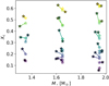 |
Fig. 7. Mass and Xc values of the benchmark models (open symbols) and the corresponding retrieved values from the best-fitting model computed with C-3PO (filled symbols). For the benchmark models Z = 0.014 and fov ∈ [0.0175, 0.0225]. |
3.2. Observational benchmark
One of the stars in our sample, KIC 9751996, has been analysed by Mombarg et al. (2020) who modelled the star using models both with and without atomic diffusion (including radiative levitation). As mentioned before, in this paper we use the same input physics in our models compared to their grid without atomic diffusion. It should be noted, however, that in this work only the periods of the prograde mode are modelled, whereas in Mombarg et al. (2020) the periods of the retrograde, zonal, and prograde are modelled simultaneously.
This yields  , and
, and  , which are consistent with the values found by Mombarg et al. (2020). The predicted period spacing pattern of this best-fitting model from C-3PO is shown in Fig. 8.
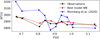 |
Fig. 8. Observed period spacing pattern of KIC 9751996 from Van Reeth et al. (2016) (black dots, prograde dipole mode only) and the best-fitting pattern predicted with C-3PO (red dots). For comparison, the solution from Mombarg et al. (2020) without atomic diffusion (their model M01) is also shown (blue dots). The observational uncertainties are typically smaller than the symbol size. |
4. Application to the sample
For all 37 stars in our sample, we apply the modelling scheme discussed in Sect. 3 to constrain M⋆, Xc, and fov in order to compare the results with those based on Π0 obtained by Mombarg et al. (2019). We recall that our aim is not to achieve good fits to the dips in the patterns, as this requires stratified envelope mixing profiles (Pedersen et al. 2021). Here we merely wish to compare the capacity of the NN with previous modelling based on actual equilibrium models rather than a numerical NN approximation thereof.
Figure 9 shows the mass and Xc of the best model predicted by C-3PO for each star. As is expected from the position of the γ Dor instability strip (Dupret et al. 2004), there is a correlation between the estimated mass and age (i.e. no young more massive or old less massive stars are observed), as already found by Mombarg et al. (2019). KIC 2710594, KIC 3448365, KIC 6678174, KIC 6953103, KIC 7380501, KIC 8645874, KIC 11099031, and KIC 11294808 are stars for which a particularly complicated period spacing pattern is observed (i.e. large deviations in the observed morphology occur compared to what we expect from the pulsation models limited to the physics described in this work). For these stars, part of the pattern has not been taken into account in the fitting. In the cases of KIC 5522154, KIC 5708550, KIC 6678174, KIC 6953103, and KIC 7365537, the best solutions to the observed mode periods do not seem to be in agreement with the photospheric observables. The former and latter are fast rotators (frot > 2.15 d−1; Van Reeth et al. 2016), and hence the inferred Teff could suffer a larger systemic error due to the larger uncertainty of the spectrum normalisation and gravity darkening. For the other three stars, it is primarily the luminosity that does not agree with the observed pulsations. For these five stars no 2σ cutoff in L, Teff, and log g is imposed, resulting in a larger uncertainty on M⋆ and Xc, as can be seen in Fig. 9.
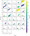 |
Fig. 9. Correlation structure of the 68% confidence intervals of M⋆ and Xc/Xini for all 37 stars in our sample from modelling the dipole period spacing patterns with C-3PO. The MLE is indicated by the red dot. The KIC number is indicated in the bottom right corner of each plot. |
We have investigated the effect of adding the rotation frequency (within the observational uncertainties) as an additional free parameter in the fitting on the MLEs. For both the fastest rotating star (KIC 12066947) and the star with the least precisely determined rotation rate (KIC 6678174), fixing the rotation rate in the modelling yields consistent estimates of the varied stellar parameters, compared to when we allow it to vary.
In addition to the (ℓ,m) = (1, 1) modes, Van Reeth et al. (2016) also observed (ℓ,m) = (1, 0) modes for KIC 4846809 and KIC 9595743 and an (ℓ,m) = (2, 2) mode for KIC 11294808. The additional period spacing patterns of these three stars are also taken into account in Step 5 of the modelling scheme (Sect. 3).
Table 3 lists the parameters of the best models found by C-3PO and of the best-fitting GYRE model. In Appendix D we show the theoretically predicted period spacing patterns for all stars in our sample, as well as the distribution of radial orders, similar to the result from Li et al. (2020). Moreover, the Brunt–Väisälä frequency profiles of the best-fitting models are shown in Fig. D.39. In many cases we are not able to reproduce the wiggly characteristics of the observed patterns, indicating that the physics used in this work is still incomplete and requires improvement. Therefore, these deviations between the patterns from our best solution and those found in the observations offer a fruitful guide to future studies with the aim of explaining the morphology of the patterns, by means of different core-boundary mixing prescriptions and/or introducing stratified envelope mixing profiles. In order to guide these future studies, we focus on one of the stars in our sample (KIC 11294808) which shows clear ‘wiggles’ in its observed period spacing patterns. With the overshoot prescription used in this work (Eq. (1)), such wiggles are only observed in our models at a level of D0 = 0.05 cm2 s−1 (see Fig. E.1). The same conclusion is found for this star when we recompute the MESA and GYRE models, but this time using a step-like penetrative convection prescription as convective-boundary mixing prescription, where we explore αov ∈ [0.05, 0.35; 0.05] (other parameter ranges kept the same). We obtain the same best model as for an exponential core overshoot in terms of mass and evolutionary stage. This corresponding best convective penetration model has a value of αov that is ten times the value of fov, in agreement with previous studies where such comparisons were made (Moravveji et al. 2016). This solution is also shown in Fig. D.30 (grey open circles).
Parameters of the best-fitting MESA/GYRE models.
The remaining differences between the observed and predicted mode periods via the NN seen in most of the stars is due to the lack of stratified envelope mixing. As shown by Pedersen et al. (2021), this causes structure to occur in the patterns. The structure can have various physical causes, for example atomic diffusion with radiative levitation (e.g. Deal et al. 2020; Mombarg et al. 2020); magnetism, which causes saw-tooth like features (e.g. Prat et al. 2019; Van Beeck et al. 2020); shear instabilities due to rotation or wave mixing (Pedersen et al. 2021); or non-linear effects (discussed below). Our results open the way to include these types of phenomena by modelling the residuals between the periods predicted by the current initial NN and the observed ones.
As an extra sanity check to assess the quality of the NN solution, we show in Fig. 10 the Π0 value derived from our best model and compare it to the observational values from Van Reeth et al. (2016, 2018) as derived from the mode identification along with the near-core rotation frequency. In general, we find adequate correspondence between the two ways of estimating Π0. The most significant discrepancy is found in KIC 11099031 (data point indicated in red). This is one of stars for which Christophe et al. (2018) found a much lower value of Π0, compared to Van Reeth et al. (2016) (see Fig. 5 in Ouazzani et al. 2019).
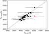 |
Fig. 10. Comparison between the Π0 values derived by Van Reeth et al. (2016, 2018) (Π0, obs, simultaneously with frot) vs. the values found from the best models presented in Table 3 of this paper (Π0, model). The grey dashed line indicates perfect correspondence. The outlier KIC 11099031 is indicated in red. |
4.1. The possible origins of CBM
The parameters of the best-fitting models discussed in this section are those extracted from the MESA and GYRE models computed in Step 5 of the modelling scheme. As illustrated in Fig. 11, the modelling of individual pulsations instead of the method employed by Mombarg et al. (2019) provides a better constraint on fov as the individual mode periods lead to less degeneracy with respect to the stellar mass and age. In addition, the luminosity is in general more precisely determined than log g for F-type stars, which further reduces the degeneracy between the stellar mass and age. The overshoot parameter has been asteroseismically calibrated for eight solar-like oscillators with a convective core by Deheuvels et al. (2016), covering a mass range from roughly 1.1 to 1.45 M⊙. They observe an increase in the overshoot parameter with increasing mass, although this trend is much less pronounced for M⋆ > 1.25 M⊙. The results from Deheuvels et al. (2016) for models with microscopic diffusion are shown in Fig. 11 (in grey). To convert from a step-like overshoot (penetrative, αov) to the exponential overshoot (diffusive) parametrizaton used in this work, we use the approximation αov ≈ 10fov inferred by Claret & Torres (2017). A similar correlation between overshooting and the mass was found by these authors from isochrone fitting of binary systems, plateauing to a value of ∼0.0175 for M⋆ ≳ 2.0 M⊙.
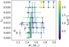 |
Fig. 11. Derived masses and overshoot parameters for all stars in our sample from the GYRE models. For comparison, the inferred overshoot parameters of low-mass stars by Deheuvels et al. (2016) (solutions with microscopic diffusion, where we have used αov ≈ 10fov) are plotted in grey. |
For the single stars modelled in this work, however, we do not observe such a mass–overshoot relation, even though a much smaller range in mass is probed. Furthermore, for a significant portion of the sample, we obtain higher values for fov than those from Claret & Torres (2017). Caution is advised when comparing overshoot values between different studies; the exact location in the star where the overshoot (core boundary mixing; CBM) profile starts is set by an additional parameter, f0, normalised by the local pressure scale height, for which we use 0.005 in this work. In Fig. 12, the extent of the overshoot zone is plotted against Xc/Xini. The size of the overshoot region is defined as the difference between rov and rcc, where rcc is defined as the radius where the temperature gradient transitions from adiabatic to radiative, and rov is the radius where the overshoot zone ends (cf. Fig. 1). No evident correlation is observed between the extent of the overshoot zone and the evolutionary stage, although the most evolved stars in our sample typically have smaller overshoot zones. It should be noted that if the value of fov is dependent on the stellar age, this is not taken into account in the current SSE models. The modelling of period spacing patterns does not probe the value of fov at the current age of the star, but rather the constant value that is needed to have the correct core properties at the age when the observations were taken. As illustrated in Fig. 13, we observe a correlation between the core mass (mcc) and the extent of the overshoot region. An increase in rov − rcc with increasing mcc is observed where there is an offset between younger and older stars. For the less massive stars, the convective core grows in mass at first, whilst for the more massive stars, the core recedes throughout the MS (see Fig. 2 in Mombarg et al. 2019). This suggests that the correlation between rov − rcc and mcc is dependent on the core density. The fractional core mass versus the stellar mass is shown in Fig. 14.
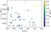 |
Fig. 12. Extent of the overshoot zone plotted against Xc/Xini. |
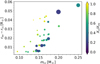 |
Fig. 13. Correlation between the convective core mass and extent of the overshoot zone. The symbol size is indicative of the mass. |
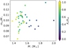 |
Fig. 14. Derived fractional convective core mass vs stellar mass. |
Although we refer to fov as the convective core overshoot parameter, fov encompasses all forms of mixing occurring close to the core boundary. If CMB is induced via rotational shears between the core and the envelope, a dependence between the amount of CMB and the rotation rate is expected. In Fig. 15 the inferred extent of the overshoot zone relative to the core size is plotted as a function of the near-core rotation rate from Van Reeth et al. (2016) (Ω = 2πfrot), scaled by  , where G is the gravitational constant. No evidence is found that the CMB increases with a faster rotating near-core region1. To fully rule out the connection between rotation and the extent of the overshoot zone, the rotation of the convective core itself needs to be measured. Saio et al. (2021) have derived the rotation of the convective core in 16 rapidly rotating γ Dor stars from the sample of Li et al. (2020) by studying the coupling between inertial modes in the convective core and g modes in the radiative envelope. These authors find only small differences with the rotation rates derived from g modes in the TAR framework for the majority of stars.
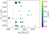 |
Fig. 15. Extent of the overshoot region with respect to the radius of the convective core as a function of the angular rotation rates from Van Reeth et al. (2016), scaled with frequency |

4.2. Angular momentum of the sample
The AM of a star, J, is defined as
 (10)
(10)
For eight stars in our sample, Van Reeth et al. (2018) have measured the ratio of the near-core rotation rate to the surface rotation rate, suggesting that all eight stars are quasi-rigidly rotating. In addition, Saio et al. (2021) find the γ Dor stars in their sample to be rotating nearly uniformly as well. Therefore, assuming Ω(r) is constant throughout the star and that typical mass loss in F-type stars (Ṁ ≃ 10−13 M⊙ yr−1) is too small to carry away significant amounts of AM from the star, we can infer the rotation rate at any point in time since J is constant. Figure 16 shows the fraction of AM in the convective core, compared to the total AM of the whole star, J, as a function of stellar age τ. Furthermore, two examples of the evolution of the AM of the convective core2, Jcc/J for KIC 2710594 (∼1.5 M⊙) and KIC 7434470 (∼1.9 M⊙) when rigid rotation is assumed, are shown.
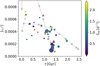 |
Fig. 16. Fractional AM of the convective core to total AM, assuming rigid rotation throughout the MS. Stars with detected Rossby modes are plotted as triangles and highlighted in red. The symbol size is indicative of the mass. The grey symbols indicate the predicted evolution of Jcc/J (assuming rigid rotation) for KIC 2710594 (upward triangles) and KIC 6953103 (downward triangles). |
Mombarg et al. (2019) observed that stars with detected Rossby modes are situated across the entire MS (based on Xc/Xini), which is in line with our findings. In Fig. 17 we show the near-core rotation as a function of absolute age τ. Stars highlighted in red are those for which Van Reeth et al. (2016) detected Rossby modes. Again, we do not find any correlation between a star’s age and the presence of Rossby modes.
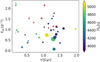 |
Fig. 17. Near-core rotation rates (and Π0) from Van Reeth et al. (2016, 2018) as a function of age τ (this work). Stars with detected Rossby modes are shown as red triangles. The symbol size is indicative of the mass. |
When rigid rotation is assumed, the initial rotation frequency at the start of the MS can be estimated. Figure 18 shows the distribution of the rotation frequencies near the zero age main sequence (ZAMS; i.e. not more than 3% of the initial hydrogen in the core burnt) as well as the distribution of the present rotation frequency (Van Reeth et al. 2016, 2018). While the distribution of the present-day near-core rotation frequencies corresponds to that found by Li et al. (2020), we find a broader distribution for the near-ZAMS rotation rates, which peaks around 1.8 d−1.
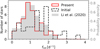 |
Fig. 18. Distributions of near-core rotation frequencies. Red: distribution of the present near-core rotation frequencies from Van Reeth et al. (2016, 2018). Black: distribution of the rotation rate near the ZAMS, assuming rigid rotation throughout the MS. Grey: normalised distribution from Li et al. (2020). |
4.3. Mode interaction in KIC 12066947
One particularly interesting star in our sample is KIC 12066947. It shows just one characteristic dip in the period spacing pattern at 0.38 days. Such a single dip is not expected to be caused by a chemical gradient because this introduces multiple dips (Miglio et al. 2008). Recently, Saio et al. (2021) were able to reproduce the sharp dip observed in the period spacing pattern of this star, using the formalism by Lee & Baraffe (1995) to compute the coupling between g modes in the radiative envelope and an inertial mode in the convective core. To exclude the scenario of constant envelope mixing combined with a chemical gradient in the core boundary layer as a possible second explanation, we again repeat Step 5 (Sect. 3), but with extremely inefficient envelope mixing: D0 = 0.05 cm2 s−1. As can be seen from the best pulsation model selected from those computed from the best stellar models according to C-3PO (see Fig. 19), a low D0 introduces a dip in the pattern around the observed dip in period spacing close to 0.38 days. However, the additional theoretically predicted dips are not observed. A rotation rate of  for KIC 12066947 has been measured by Van Reeth et al. (2016). Assuming a uniform rotation profile at 25 μHz, Ouazzani et al. (2020) have computed the radial order at which the interaction between inertial and gravito-inertial modes occurs. According to the parameters derived for KIC 12066947 in this work, the star is most similar to the mid-MS model from Ouazzani et al. (2020), for which the mode interaction is estimated to occur at npg = −44. The dip in the period spacing pattern occurs at npg = −44; therefore, if the dip is caused by interaction between gravito-inertial and pure inertial modes, it should occur close to the dip. Hence, the observed dip in the period spacing pattern of KIC 12066947 is most likely caused by mode interaction, confirming the results by Ouazzani et al. (2020) and Saio et al. (2021).
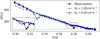 |
Fig. 19. Best-fitting model with D0 = 0.05 cm2 s−1 to the observed period spacing pattern of KIC 12066947 (black dots; Van Reeth et al. 2016). For reference, the best fit with the standard D0 = 1.0 cm2 s−1 used in this work is shown in grey. |
4.4. Comparison with Mombarg et al. (2019)
In Fig. 20 we compare the MLE for M⋆, Xc, and fov from C-3PO (this work) with those from Mombarg et al. (2019). Several key differences between the NN methodology in this work and theirs should be noted while evaluating the comparison, as summarised in Table 4. Keeping these differences in mind, the agreement among the estimated parameters is adequate, given the uncertainties on the parameter estimation. This is not the case for all stars in terms of their masses, however. The mass estimates from the NN methodology are in general lower than those of Mombarg et al. (2019). This is not a consequence of the more complex NN modelling strategy adopted here; rather, it is due to the inclusion of the stellar luminosities calculated from the Gaia DR2 data as a constraint imposed by the modelling. Figure F.1 shows the effect of including the Gaia luminosity as an extra modelling constraint on the inferred stellar mass. A systematic underestimation of the stellar masses deduced from Gaia DR2 data was also found by Pedersen et al. (2021) in their asteroseismic modelling of B-type stars. We conclude that the NN itself performs well as an asteroseismic modelling strategy, and opens the way forward for applications to large samples of γ Dor pulsators and for the use of more complex stellar models, including parametrised stratified envelope mixing profiles.
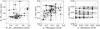 |
Fig. 20. Predictions of the C-3PO NN vs the results from Mombarg et al. (2019). The grey dashed lines indicate perfect concordance. |
Comparison between the method used in Mombarg et al. (2019) and in this work.
5. Conclusion and discussion
In this paper we have constructed a forward-modelling scheme for gravito-inertial modes in γ Dor stars, and used it to estimate the stellar mass, the central hydrogen mass fraction, and the overshooting parameter. We have eliminated the need for large grids of stellar models by training a dense neural network on a coarse grid of stellar evolution and pulsation models to predict the corresponding oscillation periods (n ∈ [15, 91]) and the luminosity, effective temperature, and surface gravity, given the mass, hydrogen mass fraction in the core, metallicity, efficiency of core-boundary mixing and radiative envelope mixing, and rotation rate. All of the input parameters of the network have been varied within appropriate ranges of γ Dor stars, making it a versatile tool for estimating stellar parameter ranges with minimal computational effort. The C-3PO neural network, comprising eight different subnetworks, has been applied to a sample of 37 γ Dor stars for which period spacing patterns have been detected by Van Reeth et al. (2016). For Teff and log g we relied on the measurements from Van Reeth et al. (2015), and have derived luminosities for the sample using Gaia DR2 distances from Bailer-Jones et al. (2018).
Using the mass and Xc estimates of C-3PO, we have computed small grids of stellar pulsation models for each star in order to further constrain the overshoot fov as well. We find no evidence that the core boundary mixing efficiency correlates with stellar mass, age, or rotation rate. However, we do observe that stars with larger core masses tend to have larger overshoot regions. Furthermore, we find that Rossby modes are only detected in the more evolved stars in our sample, which is only seen when the actual stellar age is used instead of Xc/Xini. However, a much larger sample is needed to conclude whether Rossby modes are indeed not observed for stars younger than about 1 Gyr. Li et al. (2020) compiled a sample of 611 γ Dor stars, 83 of which have observed Rossby modes. Many of these 611 stars lack spectroscopic observations; therefore, the MLEs may in general be less constrained.
To compute the mode periods we relied on the traditional approximation of rotation (TAR), which assumes spherical symmetry and loses its validity for rapidly rotating stars deformed by the centrifugal force (cf. Mathis & Prat 2019, for an improved description of the TAR in that case). In Fig. 21, the distribution of the critical Roche frequency for the stars in our sample is shown. Inspecting the quality of fit for the star with the largest fraction of Ω/Ωcrit, Roche, namely KIC 12066947 (∼80%), suggests that the TAR is still able to reproduce the observed patterns to a satisfactorily level, in line with the findings by Henneco et al. (2021). However, our models are not able the reproduce the sharp dip in the observed pattern, suggesting it is caused by resonances between gravito-inertial and pure-inertial modes (Ouazzani et al. 2020; Saio et al. 2021). An improved formalism of the TAR, taking into account the centrifugal deformation, has been developed by Mathis & Prat (2019). The inclusion of the centrifugal force in the pulsation computations of γ Dor stars has a smaller effect on the predicted values for the periods than the inclusion of stratified envelope mixing profiles due to radiative levitation (Mombarg et al. 2020) or other mixing phenomena, although for lower radial orders the effect of the centrifugal force should be observable in long time-base, space-based photometry Henneco et al. (2021).
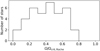 |
Fig. 21. Distribution of the rotation frequency as a fraction of the critical rotation frequency in the Roche framework. Rotation frequencies are taken from Van Reeth et al. (2016, 2018). |
In the stellar structure and evolution models used in this work, the effect of atomic diffusion is neglected. Mombarg et al. (2020) demonstrated for two slowly rotating γ Dor stars that this process (including radiative levitations) can lead to significant differences in the derived mass, age, and near-core boundary mixing. The obtained period spacing pattern of the best-fitting model for KIC 9751996 suggests that we are underestimating D0. The need for more envelope mixing supports the conclusion of Mombarg et al. (2020) who find that models without atomic diffusion better reproduce the observed mode periods for this particular star, if other forms of envelope mixing are able to counteract the effects of atomic diffusion. Even though the use of a neural network greatly decreases the number of required stellar models in the modelling, doing the full radiative levitation calculations in MESA still requires a large amount of computation time. The modelling of the sample in this work with atomic diffusion (including radiative levitation), as well as a non-constant parametrised mixing profile in the radiative envelope will be taken up in a future paper.
No scaling of Ω also does not reveal a correlation.
Jcc is computed by discretising the integral in Eq. (10), i.e.  , where i runs over the cells in the model below the convective core, and r and dm are the central radius and enclosed mass of a cell, respectively.
Acknowledgments
The research leading to these results has received funding from the European Research Council (ERC) under the European Unions Horizon 2020 research and innovation programme (grant agreement N°670519: MAMSIE) and from the KU Leuven Research Council (grant C16/18/005: PARADISE). The computational resources and services used in this work were provided by the VSC (Flemish Supercomputer Center), funded by the Research Foundation – Flanders (FWO) and the Flemish Government department EWI. TVR gratefully acknowledges support from the Research Foundation Flanders (FWO) through grant 12ZB620N. We thank Dr. Dominic M. Bowman for his comments on the manuscript.
References
- Aerts, C. 2021, Rev. Mod. Phys., 93, 015001 [Google Scholar]
- Aerts, C., Van Reeth, T., & Tkachenko, A. 2017, ApJ, 847, L7 [NASA ADS] [CrossRef] [Google Scholar]
- Aerts, C., Molenberghs, G., Michielsen, M., et al. 2018, ApJS, 237, 15 [Google Scholar]
- Aerts, C., Mathis, S., & Rogers, T. M. 2019, ARA&A, 57, 35 [NASA ADS] [CrossRef] [MathSciNet] [Google Scholar]
- Antoci, V., Cunha, M. S., Bowman, D. M., et al. 2019, MNRAS, 490, 4040 [Google Scholar]
- Asplund, M., Grevesse, N., Sauval, A. J., & Scott, P. 2009, ARA&A, 47, 481 [NASA ADS] [CrossRef] [Google Scholar]
- Bailer-Jones, C. A. L., Rybizki, J., Fouesneau, M., Mantelet, G., & Andrae, R. 2018, AJ, 156, 58 [NASA ADS] [CrossRef] [Google Scholar]
- Beck, P. G., Montalban, J., Kallinger, T., et al. 2012, Nature, 481, 55 [NASA ADS] [CrossRef] [Google Scholar]
- Bellinger, E. P., Angelou, G. C., Hekker, S., et al. 2016, ApJ, 830, 31 [Google Scholar]
- Bishop, C. 1995, Neural Networks for Pattern Recognition (USA: Oxford University Press) [Google Scholar]
- Borucki, W. J., Koch, D., Basri, G., et al. 2010, Science, 327, 977 [NASA ADS] [CrossRef] [PubMed] [Google Scholar]
- Buysschaert, B., Aerts, C., Bowman, D. M., et al. 2018, A&A, 616, A148 [NASA ADS] [CrossRef] [EDP Sciences] [Google Scholar]
- Cantiello, M., Mankovich, C., Bildsten, L., Christensen-Dalsgaard, J., & Paxton, B. 2014, ApJ, 788, 93 [Google Scholar]
- Christophe, S., Ballot, J., Ouazzani, R. M., Antoci, V., & Salmon, S. J. A. J. 2018, A&A, 618, A47 [NASA ADS] [CrossRef] [EDP Sciences] [Google Scholar]
- Claret, A., & Torres, G. 2017, ApJ, 849, 18 [Google Scholar]
- Deal, M., Goupil, M. J., Marques, J. P., Reese, D. R., & Lebreton, Y. 2020, A&A, 633, A23 [NASA ADS] [CrossRef] [EDP Sciences] [Google Scholar]
- Deheuvels, S., Brandão, I., Silva Aguirre, V., et al. 2016, A&A, 589, A93 [NASA ADS] [CrossRef] [EDP Sciences] [Google Scholar]
- den Hartogh, J. W., Eggenberger, P., & Hirschi, R. 2019, A&A, 622, A187 [NASA ADS] [CrossRef] [EDP Sciences] [Google Scholar]
- den Hartogh, J. W., Eggenberger, P., & Deheuvels, S. 2020, A&A, 634, L16 [CrossRef] [EDP Sciences] [Google Scholar]
- Dupret, M. A., Grigahcène, A., Garrido, R., Gabriel, M., & Scuflaire, R. 2004, A&A, 414, L17 [NASA ADS] [CrossRef] [EDP Sciences] [Google Scholar]
- Dupret, M.-A., Grigahcène, A., Garrido, R., et al. 2005, MNRAS, 360, 1143 [Google Scholar]
- Eckart, C. 1960, Phys. Fluids, 3, 421 [Google Scholar]
- Eggenberger, P., Lagarde, N., Miglio, A., et al. 2017, A&A, 599, A18 [NASA ADS] [CrossRef] [EDP Sciences] [Google Scholar]
- Eggenberger, P., Deheuvels, S., Miglio, A., et al. 2019a, A&A, 621, A66 [NASA ADS] [CrossRef] [EDP Sciences] [Google Scholar]
- Eggenberger, P., den Hartogh, J. W., Buldgen, G., et al. 2019b, A&A, 631, L6 [NASA ADS] [CrossRef] [EDP Sciences] [Google Scholar]
- Freytag, B., Ludwig, H. G., & Steffen, M. 1996, A&A, 313, 497 [NASA ADS] [Google Scholar]
- Fuller, J., Lecoanet, D., Cantiello, M., & Brown, B. 2014, ApJ, 796, 17 [Google Scholar]
- Fuller, J., Piro, A. L., & Jermyn, A. S. 2019, MNRAS, 485, 3661 [NASA ADS] [Google Scholar]
- Gehan, C., Mosser, B., Michel, E., Samadi, R., & Kallinger, T. 2018, A&A, 616, A24 [NASA ADS] [CrossRef] [EDP Sciences] [Google Scholar]
- Glorot, X., Bordes, A., & Bengio, Y. 2011, Proc. Mach. Learn. Res., 15, 315 [Google Scholar]
- Green, G. M., Schlafly, E. F., Finkbeiner, D., et al. 2018, MNRAS, 478, 651 [NASA ADS] [CrossRef] [Google Scholar]
- Guzik, J. A., Kaye, A. B., Bradley, P. A., Cox, A. N., & Neuforge, C. 2000, ApJ, 542, L57 [Google Scholar]
- Hendriks, L., & Aerts, C. 2019, PASP, 131, 108001 [Google Scholar]
- Henneco, J., Van Reeth, T., Prat, V., et al. 2021, A&A, 648, A97 [EDP Sciences] [Google Scholar]
- Hermes, J. J., Gänsicke, B. T., Kawaler, S. D., et al. 2017, ApJS, 232, 23 [Google Scholar]
- Hon, M., Bellinger, E. P., Hekker, S., Stello, D., & Kuszlewicz, J. S. 2020, MNRAS, 499, 2445 [Google Scholar]
- Keen, M. A., Bedding, T. R., Murphy, S. J., et al. 2015, MNRAS, 454, 1792 [Google Scholar]
- Kurtz, D. W., Saio, H., Takata, M., et al. 2014, MNRAS, 444, 102 [Google Scholar]
- Lee, U., & Baraffe, I. 1995, A&A, 301, 419 [NASA ADS] [Google Scholar]
- Li, G., Bedding, T. R., Murphy, S. J., et al. 2019, MNRAS, 482, 1757 [NASA ADS] [CrossRef] [Google Scholar]
- Li, G., Van Reeth, T., Bedding, T. R., et al. 2020, MNRAS, 491, 3586 [NASA ADS] [CrossRef] [Google Scholar]
- Maeder, A. 2009, Physics, Formation and Evolution of Rotating Stars (Berlin, Heidelberg: Springer) [Google Scholar]
- Mathis, S., & Prat, V. 2019, A&A, 631, A26 [CrossRef] [EDP Sciences] [Google Scholar]
- Michielsen, M., Pedersen, M. G., Augustson, K. C., Mathis, S., & Aerts, C. 2019, A&A, 628, A76 [NASA ADS] [CrossRef] [EDP Sciences] [Google Scholar]
- Miglio, A., Montalbán, J., Noels, A., & Eggenberger, P. 2008, MNRAS, 386, 1487 [Google Scholar]
- Mombarg, J. S. G., Van Reeth, T., Pedersen, M. G., et al. 2019, MNRAS, 485, 3248 [Google Scholar]
- Mombarg, J. S. G., Dotter, A., Van Reeth, T., et al. 2020, ApJ, 895, 51 [Google Scholar]
- Moravveji, E., Aerts, C., Pápics, P. I., Triana, S. A., & Vandoren, B. 2015, A&A, 580, A27 [NASA ADS] [CrossRef] [EDP Sciences] [Google Scholar]
- Moravveji, E., Townsend, R. H. D., Aerts, C., & Mathis, S. 2016, ApJ, 823, 130 [Google Scholar]
- Mosser, B., Goupil, M. J., Belkacem, K., et al. 2012, A&A, 548, A10 [NASA ADS] [CrossRef] [EDP Sciences] [Google Scholar]
- Ouazzani, R.-M., Salmon, S. J. A. J., Antoci, V., et al. 2017, MNRAS, 465, 2294 [Google Scholar]
- Ouazzani, R. M., Marques, J. P., Goupil, M. J., et al. 2019, A&A, 626, A121 [NASA ADS] [CrossRef] [EDP Sciences] [Google Scholar]
- Ouazzani, R.-M., Lignières, F., Dupret, M.-A., et al. 2020, A&A, 640, A49 [EDP Sciences] [Google Scholar]
- Paxton, B., Bildsten, L., Dotter, A., et al. 2011, ApJS, 192, 3 [Google Scholar]
- Paxton, B., Cantiello, M., Arras, P., et al. 2013, ApJS, 208, 4 [NASA ADS] [CrossRef] [Google Scholar]
- Paxton, B., Marchant, P., Schwab, J., et al. 2015, ApJS, 220, 15 [Google Scholar]
- Paxton, B., Schwab, J., Bauer, E. B., et al. 2018, ApJS, 234, 34 [Google Scholar]
- Paxton, B., Smolec, R., Schwab, J., et al. 2019, ApJS, 243, 10 [Google Scholar]
- Pedersen, M. G., Aerts, C., Pápics, P. I., & Rogers, T. M. 2018, A&A, 614, A128 [NASA ADS] [CrossRef] [EDP Sciences] [Google Scholar]
- Pedersen, M. G., Aerts, C., Pápics, P. I., et al. 2021, Nat. Astron., in press, http://doi.org/10.1038/s41550-021-01351-x [Google Scholar]
- Prat, V., Mathis, S., Buysschaert, B., et al. 2019, A&A, 627, A64 [NASA ADS] [CrossRef] [EDP Sciences] [Google Scholar]
- Ricker, G. R., Winn, J. N., Vanderspek, R., et al. 2015, J. Astron. Telesc. Instrum. Syst., 1, 014003 [Google Scholar]
- Rogers, T. M., & McElwaine, J. N. 2017, ApJ, 848, L1 [Google Scholar]
- Saio, H., Kurtz, D. W., Takata, M., et al. 2015, MNRAS, 447, 3264 [Google Scholar]
- Saio, H., Bedding, T. R., Kurtz, D. W., et al. 2018, MNRAS, 477, 2183 [Google Scholar]
- Saio, H., Takata, M., Lee, U., Li, G., & Van Reeth, T. 2021, MNRAS, 502, 5856 [Google Scholar]
- Salaris, M., & Cassisi, S. 2017, R. Soc. Open Sci., 4, 170192 [Google Scholar]
- Tayar, J., & Pinsonneault, M. H. 2018, ApJ, 868, 150 [Google Scholar]
- Torres, G. 2010, AJ, 140, 1158 [NASA ADS] [CrossRef] [Google Scholar]
- Townsend, R. H. D. 2003, MNRAS, 340, 1020 [Google Scholar]
- Townsend, R. H. D., & Teitler, S. A. 2013, MNRAS, 435, 3406 [NASA ADS] [CrossRef] [Google Scholar]
- Townsend, R. H. D., Goldstein, J., & Zweibel, E. G. 2018, MNRAS, 475, 879 [Google Scholar]
- Van Beeck, J., Prat, V., Van Reeth, T., et al. 2020, A&A, 638, A149 [EDP Sciences] [Google Scholar]
- Van Reeth, T., Tkachenko, A., Aerts, C., et al. 2015, ApJS, 218, 27 [Google Scholar]
- Van Reeth, T., Tkachenko, A., & Aerts, C. 2016, A&A, 593, A120 [NASA ADS] [CrossRef] [EDP Sciences] [Google Scholar]
- Van Reeth, T., Mombarg, J. S. G., Mathis, S., et al. 2018, A&A, 618, A24 [NASA ADS] [EDP Sciences] [Google Scholar]
- Verma, K., Raodeo, K., Basu, S., et al. 2019, MNRAS, 483, 4678 [Google Scholar]
- Xiong, D. R., Deng, L., Zhang, C., & Wang, K. 2016, MNRAS, 457, 3163 [Google Scholar]
Appendix A: luminosities from Gaia
Visual apparent magnitudes mV, bolometric corrections BCV, distances D (Bailer-Jones et al. 2018), and extinctions AV used to derive the luminosity.
Appendix B: Best-fitting parameters from neural network
Best-fitting parameters of the model predicted by the C-3PO neural network.
Appendix C: Distribution of the residuals
In Fig. C.1 we show the residuals (Ptrue − Ppred), per radial order, of the NN on the grid of 38915 stellar pulsation models used for training and validation.
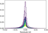 |
Fig. C.1. Normalised distributions of the residuals of the NN on the grid of pulsation models used for training and validation. Darker colors indicate higher radial orders. |
Appendix D: Best-matching period spacing patterns
In this appendix we present the best-fitting period spacing patterns found with C-3PO (in red) and GYRE (in blue) for all stars in our sample. The observed period spacing patterns are taken from Van Reeth et al. (2015), where the uncertainties are typically smaller than the symbol size. Missing radial orders are indicated by dashed lines. As only the mode periods are fitted, these values are also indicated by dashes at the bottom or top of each panel. Furthermore, in Fig. D.1 we show the distribution of radial orders. A similar distribution is found compared to the one from Li et al. (2020, their Fig. 17).
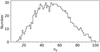 |
Fig. D.1. Distribution of the identified radial orders for all stars in our sample. |
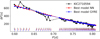 |
Fig. D.2. Best-fitting models from the neural network and GYRE for KIC 2710594. |
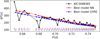 |
Fig. D.3. Best-fitting models from the neural network and GYRE for KIC 3448365. |
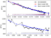 |
Fig. D.4. Best-fitting models from the neural network and GYRE for KIC 4846809. Top: (ℓ,m) = (1, 1); bottom: (ℓ,m) = (1, 0). |
 |
Fig. D.5. Best-fitting models from the neural network and GYRE for KIC 5114382. |
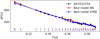 |
Fig. D.6. Best-fitting models from the neural network and GYRE for KIC 5522154. |
 |
Fig. D.7. Best-fitting models from the neural network and GYRE for KIC 5708550. |
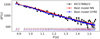 |
Fig. D.8. Best-fitting models from the neural network and GYRE for KIC 5788623. |
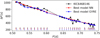 |
Fig. D.9. Best-fitting models from the neural network and GYRE for KIC 6468146. |
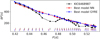 |
Fig. D.10. Best-fitting models from the neural network and GYRE for KIC 6468987. |
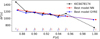 |
Fig. D.11. Best-fitting models from the neural network and GYRE for KIC 6678174. |
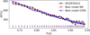 |
Fig. D.12. Best-fitting models from the neural network and GYRE for KIC 6935014. |
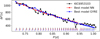 |
Fig. D.13. Best-fitting models from the neural network and GYRE for KIC 6953103. |
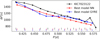 |
Fig. D.14. Best-fitting models from the neural network and GYRE for KIC 7023122. |
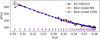 |
Fig. D.15. Best-fitting models from the neural network and GYRE for KIC 7365537. |
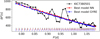 |
Fig. D.16. Best-fitting models from the neural network and GYRE for KIC 7380501. |
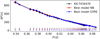 |
Fig. D.17. Best-fitting models from the neural network and GYRE for KIC 7434470. |
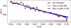 |
Fig. D.18. Best-fitting models from the neural network and GYRE for KIC 7583663. |
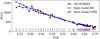 |
Fig. D.19. Best-fitting models from the neural network and GYRE for KIC 7939065. |
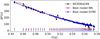 |
Fig. D.20. Best-fitting models from the neural network and GYRE for KIC 8364249. |
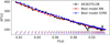 |
Fig. D.21. Best-fitting models from the neural network and GYRE for KIC 8375138. |
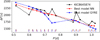 |
Fig. D.22. Best-fitting models from the neural network and GYRE for KIC 8645874. |
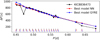 |
Fig. D.23. Best-fitting models from the neural network and GYRE for KIC 8836473. |
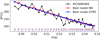 |
Fig. D.24. Best-fitting models from the neural network and GYRE for KIC 9480469. |
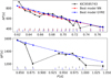 |
Fig. D.25. Best-fitting models from the neural network and GYRE for KIC 9595743. Top: (ℓ,m) = (1, 1); bottom: (ℓ,m) = (1, 0). |
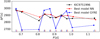 |
Fig. D.26. Best-fitting models from the neural network and GYRE for KIC 9751996. |
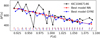 |
Fig. D.27. Best-fitting models from the neural network and GYRE for KIC 10467146. |
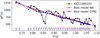 |
Fig. D.28. Best-fitting models from the neural network and GYRE for KIC 11080103. |
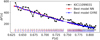 |
Fig. D.29. Best-fitting models from the neural network and GYRE for KIC 11099031. |
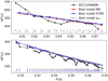 |
Fig. D.30. Best-fitting models from the neural network and GYRE for KIC 11294808. Top: (ℓ,m) = (1, 1); bottom: (ℓ,m) = (2, 2). Additionally, the best-fitting GYRE model based on equilibrium models with a step-like core overshoot prescription is shown in grey. |
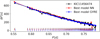 |
Fig. D.31. Best-fitting models from the neural network and GYRE for KIC 11456474. |
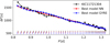 |
Fig. D.32. Best-fitting models from the neural network and GYRE for KIC 11721304. |
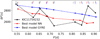 |
Fig. D.33. Best-fitting models from the neural network and GYRE for KIC 11754232. |
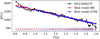 |
Fig. D.34. Best-fitting models from the neural network and GYRE for KIC 11826272. |
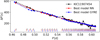 |
Fig. D.35. Best-fitting models from the neural network and GYRE for KIC 11907454. |
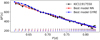 |
Fig. D.36. Best-fitting models from the neural network and GYRE for KIC 11917550. |
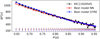 |
Fig. D.37. Best-fitting models from the neural network and GYRE for KIC 11920505. |
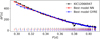 |
Fig. D.38. Best-fitting models from the neural network and GYRE for KIC 12066947. |
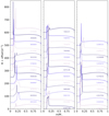 |
Fig. D.39. Brunt–Väisälä frequency profiles of the best model for each star in our sample. For clarity, the profiles are offset by 50 d−1 from one another. |
Appendix E: Test with D0 = 0.05 cm2 s−1
In this appendix we show the result of the modelling of KIC 11294808, where we have fixed D0 = 0.05 cm2 s−1 instead of D0 = 1 cm2 s−1 used in the rest of the paper.
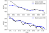 |
Fig. E.1. Best-fitting GYRE model for KIC 11294808, when D0 = 0.05 cm2 s−1 is assumed. Top: (ℓ,m) = (1, 1); bottom: (ℓ,m) = (2, 2). |
Appendix F: Effect of including Gaia luminosities on the derived mass
In Fig. F.1, we show the difference in inferred stellar mass when we do not include the luminosity from Gaia DR2 in our modelling procedure.
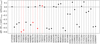 |
Fig. F.1. Differences in inferred mass per star (KIC ID on the abscissa) when the luminosities of the models are not required to comply with the observed luminosity deduced from Gaia DR2 data. Constraints on Teff and log g are in both cases enforced. The stars for which we have not used the Gaia luminosity in the modelling are indicated in red. For these stars we have put no constraints on the spectroscopic parameters in our final MLE (hence this solution is not indicated here). |
All Tables
Visual apparent magnitudes mV, bolometric corrections BCV, distances D (Bailer-Jones et al. 2018), and extinctions AV used to derive the luminosity.
All Figures
|
Fig. 1. Chemical mixing profile showing the different mixing zones in a model for an intermediate-mass star. The ordinate shows the local efficiency of chemical (diffusive) mixing. The thin outer convection zone is not shown in the plot. The radii of the convective core boundary (rcc) and overshoot zone (rov) are also indicated. Mixing inside the convective regions is based on MLT and occurs instantaneously. The red dashed line slightly to the left of rcc/R⋆ indicates the starting point of the overshoot zone (r0 in Eq. (1)). |
| In the text | |
|
Fig. 2. Schematic overview of the configuration of the dense neural network trained to predict the periods of the (ℓ, m) = (1,1) modes for a given θ = (M⋆, Xc, Z, fov, D0, frot, M⋆ ⋅ Xc, M⋆ ⋅ Z). The values of the input parameters are transformed following Eq. (2). |
| In the text | |
|
Fig. 3. Loss (mean squared error + L2 regularisation term) as a function of epoch. The NNs training on the pulsation models (bottom panel) reached an optimal solution within the maximum number of epochs. In all cases a similar loss is obtained for the training and validation sets, indicating the NNs were able to generalise the synaptic weights. |
| In the text | |
|
Fig. 4. Positions in the Hertzsprung-Russel diagram of all stars in our sample. The values of Teff and Π0 are taken from Van Reeth et al. (2016). The evolution tracks shown are for Z = 0.014 and fov = 0.0175. For the stars marked with red circles no reliable extinction estimate could be made because they are too close to the Sun, and therefore their interstellar extinction values are close to zero. |
| In the text | |
|
Fig. 5. Comparison between the predictions of C-3PO (dots) and the MESA benchmark evolution tracks (solid lines) for Z = 0.012 and Z = 0.023. The predictions are sampled from Xc = 0.70 to 0.05 with a step size of 0.05. |
| In the text | |
|
Fig. 6. Examples of the recovered mass and Xc of two benchmark models (white stars: input; red stars: best model predicted by NN). Although the period spacings of trapped modes are more difficult to predict (bottom panel), the inclusion of the photospheric observables yields accurate predictions of the mass and Xc. Middle panels: sampling density is increased in the parameter space where the predicted photospheric observables comply with those of the input model (see Sect. 3). Model 1: (M⋆, Xc, Z, fov, D0, frot) = (1.35 M⊙, 0.515, 0.014, 0.0225, 1 cm2 s−1, 0.7457 d−1). Model 2: (M⋆, Xc, Z, fov, D0, frot) = (1.95 M⊙, 0.08, 0.014, 0.0225, 1 cm2 s−1, 0.0449 d−1). Typical uncertainties on ΔP are of the order of several tens of seconds. |
| In the text | |
|
Fig. 7. Mass and Xc values of the benchmark models (open symbols) and the corresponding retrieved values from the best-fitting model computed with C-3PO (filled symbols). For the benchmark models Z = 0.014 and fov ∈ [0.0175, 0.0225]. |
| In the text | |
|
Fig. 8. Observed period spacing pattern of KIC 9751996 from Van Reeth et al. (2016) (black dots, prograde dipole mode only) and the best-fitting pattern predicted with C-3PO (red dots). For comparison, the solution from Mombarg et al. (2020) without atomic diffusion (their model M01) is also shown (blue dots). The observational uncertainties are typically smaller than the symbol size. |
| In the text | |
|
Fig. 9. Correlation structure of the 68% confidence intervals of M⋆ and Xc/Xini for all 37 stars in our sample from modelling the dipole period spacing patterns with C-3PO. The MLE is indicated by the red dot. The KIC number is indicated in the bottom right corner of each plot. |
| In the text | |
|
Fig. 10. Comparison between the Π0 values derived by Van Reeth et al. (2016, 2018) (Π0, obs, simultaneously with frot) vs. the values found from the best models presented in Table 3 of this paper (Π0, model). The grey dashed line indicates perfect correspondence. The outlier KIC 11099031 is indicated in red. |
| In the text | |
|
Fig. 11. Derived masses and overshoot parameters for all stars in our sample from the GYRE models. For comparison, the inferred overshoot parameters of low-mass stars by Deheuvels et al. (2016) (solutions with microscopic diffusion, where we have used αov ≈ 10fov) are plotted in grey. |
| In the text | |
|
Fig. 12. Extent of the overshoot zone plotted against Xc/Xini. |
| In the text | |
|
Fig. 13. Correlation between the convective core mass and extent of the overshoot zone. The symbol size is indicative of the mass. |
| In the text | |
|
Fig. 14. Derived fractional convective core mass vs stellar mass. |
| In the text | |
|
Fig. 15. Extent of the overshoot region with respect to the radius of the convective core as a function of the angular rotation rates from Van Reeth et al. (2016), scaled with frequency |
| In the text | |
|
Fig. 16. Fractional AM of the convective core to total AM, assuming rigid rotation throughout the MS. Stars with detected Rossby modes are plotted as triangles and highlighted in red. The symbol size is indicative of the mass. The grey symbols indicate the predicted evolution of Jcc/J (assuming rigid rotation) for KIC 2710594 (upward triangles) and KIC 6953103 (downward triangles). |
| In the text | |
|
Fig. 17. Near-core rotation rates (and Π0) from Van Reeth et al. (2016, 2018) as a function of age τ (this work). Stars with detected Rossby modes are shown as red triangles. The symbol size is indicative of the mass. |
| In the text | |
|
Fig. 18. Distributions of near-core rotation frequencies. Red: distribution of the present near-core rotation frequencies from Van Reeth et al. (2016, 2018). Black: distribution of the rotation rate near the ZAMS, assuming rigid rotation throughout the MS. Grey: normalised distribution from Li et al. (2020). |
| In the text | |
|
Fig. 19. Best-fitting model with D0 = 0.05 cm2 s−1 to the observed period spacing pattern of KIC 12066947 (black dots; Van Reeth et al. 2016). For reference, the best fit with the standard D0 = 1.0 cm2 s−1 used in this work is shown in grey. |
| In the text | |
|
Fig. 20. Predictions of the C-3PO NN vs the results from Mombarg et al. (2019). The grey dashed lines indicate perfect concordance. |
| In the text | |
|
Fig. 21. Distribution of the rotation frequency as a fraction of the critical rotation frequency in the Roche framework. Rotation frequencies are taken from Van Reeth et al. (2016, 2018). |
| In the text | |
|
Fig. C.1. Normalised distributions of the residuals of the NN on the grid of pulsation models used for training and validation. Darker colors indicate higher radial orders. |
| In the text | |
|
Fig. D.1. Distribution of the identified radial orders for all stars in our sample. |
| In the text | |
|
Fig. D.2. Best-fitting models from the neural network and GYRE for KIC 2710594. |
| In the text | |
|
Fig. D.3. Best-fitting models from the neural network and GYRE for KIC 3448365. |
| In the text | |
|
Fig. D.4. Best-fitting models from the neural network and GYRE for KIC 4846809. Top: (ℓ,m) = (1, 1); bottom: (ℓ,m) = (1, 0). |
| In the text | |
|
Fig. D.5. Best-fitting models from the neural network and GYRE for KIC 5114382. |
| In the text | |
|
Fig. D.6. Best-fitting models from the neural network and GYRE for KIC 5522154. |
| In the text | |
|
Fig. D.7. Best-fitting models from the neural network and GYRE for KIC 5708550. |
| In the text | |
|
Fig. D.8. Best-fitting models from the neural network and GYRE for KIC 5788623. |
| In the text | |
|
Fig. D.9. Best-fitting models from the neural network and GYRE for KIC 6468146. |
| In the text | |
|
Fig. D.10. Best-fitting models from the neural network and GYRE for KIC 6468987. |
| In the text | |
|
Fig. D.11. Best-fitting models from the neural network and GYRE for KIC 6678174. |
| In the text | |
|
Fig. D.12. Best-fitting models from the neural network and GYRE for KIC 6935014. |
| In the text | |
|
Fig. D.13. Best-fitting models from the neural network and GYRE for KIC 6953103. |
| In the text | |
|
Fig. D.14. Best-fitting models from the neural network and GYRE for KIC 7023122. |
| In the text | |
|
Fig. D.15. Best-fitting models from the neural network and GYRE for KIC 7365537. |
| In the text | |
|
Fig. D.16. Best-fitting models from the neural network and GYRE for KIC 7380501. |
| In the text | |
|
Fig. D.17. Best-fitting models from the neural network and GYRE for KIC 7434470. |
| In the text | |
|
Fig. D.18. Best-fitting models from the neural network and GYRE for KIC 7583663. |
| In the text | |
|
Fig. D.19. Best-fitting models from the neural network and GYRE for KIC 7939065. |
| In the text | |
|
Fig. D.20. Best-fitting models from the neural network and GYRE for KIC 8364249. |
| In the text | |
|
Fig. D.21. Best-fitting models from the neural network and GYRE for KIC 8375138. |
| In the text | |
|
Fig. D.22. Best-fitting models from the neural network and GYRE for KIC 8645874. |
| In the text | |
|
Fig. D.23. Best-fitting models from the neural network and GYRE for KIC 8836473. |
| In the text | |
|
Fig. D.24. Best-fitting models from the neural network and GYRE for KIC 9480469. |
| In the text | |
|
Fig. D.25. Best-fitting models from the neural network and GYRE for KIC 9595743. Top: (ℓ,m) = (1, 1); bottom: (ℓ,m) = (1, 0). |
| In the text | |
|
Fig. D.26. Best-fitting models from the neural network and GYRE for KIC 9751996. |
| In the text | |
|
Fig. D.27. Best-fitting models from the neural network and GYRE for KIC 10467146. |
| In the text | |
|
Fig. D.28. Best-fitting models from the neural network and GYRE for KIC 11080103. |
| In the text | |
|
Fig. D.29. Best-fitting models from the neural network and GYRE for KIC 11099031. |
| In the text | |
|
Fig. D.30. Best-fitting models from the neural network and GYRE for KIC 11294808. Top: (ℓ,m) = (1, 1); bottom: (ℓ,m) = (2, 2). Additionally, the best-fitting GYRE model based on equilibrium models with a step-like core overshoot prescription is shown in grey. |
| In the text | |
|
Fig. D.31. Best-fitting models from the neural network and GYRE for KIC 11456474. |
| In the text | |
|
Fig. D.32. Best-fitting models from the neural network and GYRE for KIC 11721304. |
| In the text | |
|
Fig. D.33. Best-fitting models from the neural network and GYRE for KIC 11754232. |
| In the text | |
|
Fig. D.34. Best-fitting models from the neural network and GYRE for KIC 11826272. |
| In the text | |
|
Fig. D.35. Best-fitting models from the neural network and GYRE for KIC 11907454. |
| In the text | |
|
Fig. D.36. Best-fitting models from the neural network and GYRE for KIC 11917550. |
| In the text | |
|
Fig. D.37. Best-fitting models from the neural network and GYRE for KIC 11920505. |
| In the text | |
|
Fig. D.38. Best-fitting models from the neural network and GYRE for KIC 12066947. |
| In the text | |
|
Fig. D.39. Brunt–Väisälä frequency profiles of the best model for each star in our sample. For clarity, the profiles are offset by 50 d−1 from one another. |
| In the text | |
|
Fig. E.1. Best-fitting GYRE model for KIC 11294808, when D0 = 0.05 cm2 s−1 is assumed. Top: (ℓ,m) = (1, 1); bottom: (ℓ,m) = (2, 2). |
| In the text | |
|
Fig. F.1. Differences in inferred mass per star (KIC ID on the abscissa) when the luminosities of the models are not required to comply with the observed luminosity deduced from Gaia DR2 data. Constraints on Teff and log g are in both cases enforced. The stars for which we have not used the Gaia luminosity in the modelling are indicated in red. For these stars we have put no constraints on the spectroscopic parameters in our final MLE (hence this solution is not indicated here). |
| In the text | |
Current usage metrics show cumulative count of Article Views (full-text article views including HTML views, PDF and ePub downloads, according to the available data) and Abstracts Views on Vision4Press platform.
Data correspond to usage on the plateform after 2015. The current usage metrics is available 48-96 hours after online publication and is updated daily on week days.
Initial download of the metrics may take a while.