| Issue |
A&A
Volume 650, June 2021
Parker Solar Probe: Ushering a new frontier in space exploration
|
|
|---|---|---|
| Article Number | A7 | |
| Number of page(s) | 10 | |
| Section | The Sun and the Heliosphere | |
| DOI | https://doi.org/10.1051/0004-6361/202039514 | |
| Published online | 02 June 2021 | |
The active region source of a type III radio storm observed by Parker Solar Probe during encounter 2
1
PMOD/WRC,
Dorfstrasse 33
7260
Davos Dorf,
Switzerland
e-mail: louise.harra@pmodwrc.ch
2
ETH-Zurich,
Hönggerberg campus, HIT building,
Zürich, Switzerland
3
College of Science, George Mason University, 4400 University Drive,
Fairfax,
VA 22030,
USA
e-mail: dhbrooks.work@gmail.com
4
Physics Department and Space Sciences Laboratory, University of California,
Berkeley,
USA
e-mail: bale@berkeley.edu
5
Instituto de Astronomía y Física del Espacio (IAFE),
CONICET-UBA,
Buenos Aires, Argentina
6
Facultad de Ciencias Exactas y Naturales (FCEN),
UBA,
Buenos Aires, Argentina
7
Fachhochschule Nordwestschweiz (FHNW),
Bahnhofstrasse 6,
5210
Windisch, Switzerland
8
Universidad Nacional de Colombia, Observatorio Astronómico Nacional,
Bogotá, Colombia
Received:
24
September
2020
Accepted:
8
February
2021
Context. We investigated the source of a type III radio burst storm during encounter 2 of NASA’s Parker Solar Probe (PSP) mission.
Aims. It was observed that in encounter 2 of NASA’s PSP mission there was a large amount of radio activity and, in particular, a noise storm of frequent, small type III bursts from 31 March to 6 April 2019. Our aim is to investigate the source of these small and frequent bursts.
Methods. In order to do this, we analysed data from the Hinode EUV Imaging Spectrometer, PSP FIELDS, and the Solar Dynamics Observatory Atmospheric Imaging Assembly. We studied the behaviour of active region 12737, whose emergence and evolution coincides with the timing of the radio noise storm and determined the possible origins of the electron beams within the active region. To do this, we probed the dynamics, Doppler velocity, non-thermal velocity, FIP bias, and densities, and carried out magnetic modelling.
Results. We demonstrate that although the active region on the disc produces no significant flares, its evolution indicates it is a source of the electron beams causing the radio storm. They most likely originate from the area at the edge of the active region that shows strong blue-shifted plasma. We demonstrate that as the active region grows and expands, the area of the blue-shifted region at the edge increases, which is also consistent with the increasing area where large-scale or expanding magnetic field lines from our modelling are anchored. This expansion is most significant between 1 and 4 April 2019, coinciding with the onset of the type III storm and the decrease of the individual burst’s peak frequency, indicating that the height at which the peak radiation is emitted increases as the active region evolves.
Key words: Sun: corona / solar wind / Sun: radio radiation / Sun: abundances / Sun: atmosphere
© ESO 2021
1 Introduction
Type III radio bursts are observed regularly on the Sun, and their sources are beams of energetic electrons streaming outwards along open magnetic field lines. The largest solar energetic particle (SEP) events are due to shocks associated with coronal mass ejections (CME) and solar flares, according to Reames (2017) for instance, though others can be associated with jets. For example, Krucker et al. (2011) made a study of jets associated with flares as sources of supra-thermal electron beams. The flares in this paper all had energies higher than a C2 GOES classification. However, electrons can be accelerated in smaller energy release events in active regions, when a magnetic field in a coronal hole interacts with a nearby closed magnetic field, and even in bright points that produce jets (see the review by Reid & Ratcliffe 2014).
NASA’s Parker Solar Probe (PSP) mission has opened up a new way of probing type III bursts due to the close vicinity to the Sun. Pulupa et al. (2020) have explored the statistics of type III bursts during the first two encounters of PSP. They found that only a few bursts occurred during encounter 1 (E01, October-November 2018, perihelion 6 November 2018), during which there was minimal solar activity. In encounter 2 (E02, March-April 2019, perihelion 4 April 2019), however, there were a number of dynamic active regions, and a large number of type III radio bursts were observed by PSP. In particular, two active regions (AR 12 737 and AR 12 738) were prominent during this time interval and at solar locations such that radio waves would likely reach PSP. AR 12 738 was the larger active region, receiving its NOAA designation on 6 April as it rotated onto the solar disc as viewed from Earth, but it had existed at least 2 weeks prior and was visible in STEREO A/SECCHI data. Krupar et al. (2020) used radio triangulation of a single strong radio burst on 3 April and show its location to be consistent with a Parker spiral emerging from AR 12738, indicating it was responsible for at least some of the radio activity observed at this time. In addition, Cattell et al. (2021), find some evidence of correlating periodicities in AR 12738 and in radio at PSP, although the interval they investigated is well after the time period studied in this paper, once AR 12738 had rotated on disc and AR 12737 had rotated off disc.
AR 12737, meanwhile, was observed to develop out of a coronal bright point near the east limb on 31 March and to evolve and grow before reaching a more steady state on approximately 6 April. At this time, in addition to strong impulsive bursts which PSP measured throughout this encounter and which Krupar et al. (2020) were able to associate with the larger active region, a significant type III radio noise storm occurred consisting of a huge number of smaller and more quickly repeating radio bursts. In addition, this noise storm showed the interesting feature of a systematic decrease in peak frequency with time at the exact time that AR 12737 was emerging and developing. This will bediscussed further in relation to Fig. 1, but here we simply state that for the above reasons, it is well motivated to study this active region in relation to the noise storm as this time. In addition, in contrast to the larger active region, AR 12737 is visible on disc during PSP’s closest approach to the Sun (4 April), and thus it is more likely to measure weaker radio events which are harder to study at 1 AU. Hence AR 12737 is observed at this time with all the available Earth-based instrumentation including imaging spectroscopy, radio interferometry, magnetographs, and more. Since the active region is not flare active during our period of interest, we consider other possible sources of the type III bursts. Other possibilities are jets, micro-flares, and active region outflows.
Jets are an important aspect of electron acceleration, and they indeed have been put forward as a means to explain the magnetic switchbacks that have been seen so clearly by PSP (Bale et al. 2019; Kasper et al. 2019; Horbury et al. 2020). Sterling & Moore (2020) have proposed that reconnected minifilament eruptions can manifest as outward propagating Alfvénic fluctuations that steepen into a disturbance as they move through the solar wind. Mulay et al. (2019) show a spatial association of an active region jet and the interplanetary type-III burst source that is co-spatial with extrapolated open magnetic field lines. The bunches of type-III bursts occurred before and during jet eruption, suggesting that particle acceleration begins before the extreme ultraviolet (EUV) jet eruption.
Another potential source of type III bursts are the blue-shifted regions found at the edges of active regions (e.g. Harra et al. 2008). The blue-shifted regions have been put forward as one of the potential sources of the slow solar wind, and they have been found to frequently have elemental abundances consistent with the slow solar wind (e.g. Brooks & Warren 2011). Del Zanna et al. (2011) have also studied these outflows and suggest that the continuous growth of active regions maintains a steady reconnection across the separatrices at the null point in the corona. The acceleration of electrons in the interchange reconnection region between the closed loops in the AR core and the outflow on open field lines at the boundary produces a radio noise storm in the closed loop areas, as well as weak type III emission along the open field lines.
In this paper, we explore the data from the second solar encounter of PSP (E02) around perihelion on 4 April 2019. We also investigate the possible source(s) associated with AR 12737 of the type III radio storm that occurs in the lead up to this time.
2 Instrumentation and data analysis
The Hinode EUV Imaging Spectrometer (EIS) instrument (Culhane et al. 2007) is an imaging spectrometer that has two narrow slits that can build up images through moving a mirror, and two slots. In this work we use studies with the 2′′ slit, where spectral images have been built up that cover the whole active region starting from 1 April less than a day after the region first emerged. In addition, there is a fast three-step raster with a cadence of 42 s on 1 April starting at 17:00 UT and lasting an hour. The field of view in this case covers a strip towards the eastern edge of the active region. We processed the EIS data using the standard calibration procedure eis_ prep. The emission lines were fitted with single or multiple Gaussian profiles (depending on the presence of known blends) in order to extract plasma parameters, such as Doppler velocity, non-thermal velocity, and FIP (first ionisation potential) bias.
The spectroscopic data were combined with Atmospheric Imaging Assembly (AIA) data from the Solar Dynamics Observatory (SDO; Pesnell et al. 2012) to provide context imaging and an understanding of the dynamical behaviour of the action region as it emerged on 31 March and developed through to 7 April 2019.
Measurements of interplanetary type III radio bursts were made by the Radio Frequency Spectrometer (RFS) subsystem (Pulupa et al. 2017) of the FIELDS instrument suite (Bale et al. 2016) on the NASA PSP mission (Fox et al. 2016). The FIELDS/RFS system is a base-band radio receiver that produces full Stokes parameters in the range of 10.5 kHz–19.17 MHz, corresponding to plasma frequencies at radial distances of ~1.6 RS to 1 AU (Leblanc et al. 1998). Voltage measurements are made on two ~7m crossed dipoles and digitised into two virtual receivers (the High Frequency Receiver – HFR and the Low Frequency Receiver – LFR) in 128 pseudo-log spaced (Δf∕f ≈ 4%) frequency bins with one spectrum each, lasting 7 s during normal solar encounter operations. Auto- and cross-spectra are used to produce Stokes parameters. The RFS system has good sensitivity down to the level of the galactic synchrotron spectrum (Pulupa et al. 2020) and, thus, it is capable of measuring very weak solar radio bursts.
Solar observations using the Murchison Widefield Array (MWA) were made during the period of Parker Solar Probe (PSP) perihelion. However, the observations were corrupted by incorrect pointing, except on 5 April. The Murchison Widefield Array (MWA) located in Western Australia is a new generation low-frequency radio interferometer based on a large-‘N’ design (Lonsdale et al. 2009; Tingay et al. 2013). It has 128 elements and operates between the 80 to 300 MHz frequency range. Here, we use MWA solar data from the phase-II configuration, with baselines extending up to 5 km (Wayth et al. 2018). Long baselines, accompanied by a large number of elements, make MWA suitable for studyingsmall but extended features, such as active regions. We analysed 5 min of MWA solar data from 5 April 2019 04:00:16 to 04:05:16 UT taken during the G0002 solar observation programme. The solar observations were made in ‘picket-fence’ mode, that is to say the total available bandwidth of 30.72 MHz can be distributed within 80–300 MHz in 12 roughly log-spaced chunks, each 2.56 MHz wide. Here, we analyse four frequency bands at 107.5, 163.8, 192.0, and 240.6 MHz.
Since our aim is to find the origin of the type III noise storm measured at PSP from 1 to 6 April 2019, we modelled the coronal magnetic field of AR 12737 during that period in search of large-scale or expanding field lines (i.e. ‘open’ within the limitations of a local magnetic field model approach) that could be associated with the areas where EIS observes blue-shifted regions. Our model is carried out by taking the vertical component of the photospheric magnetic field derived from SDO/HMI observations as a boundary condition. The magnetic field vertical component is computed from the line-of-sight magnetograms downloaded from the Joint Science Operation Center (JSOC1). We selected data with a 720 ms resolution from that database.
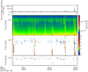 |
Fig. 1 PSP/RFS, RSTN, and MWA radio frequency measurements, AIA 193 Å intensity, and GOES X-ray data over the full interval from 30 March 2019 to 6 April 2019. Top panel: daily RSTN flux from 30 March to 6 April 2019 at 245 MHz. The red circle marks the flux at 240 MHz obtained from the MWA flux calibration, with error bars from the temporal RMS each day. Second panel: GOES soft X-ray flux data, which do not show any significant flares. Third panel: AIA 193 Å intensity integrated over the FOV shown in Fig. 3, showing the growth and flattening off of the development of the AR from 31 March to 4 April. Fourth panel: again the normalised Stokes intensity above 18 MHz and fifth panel: again the full spectrogram. Sixth panel: frequency of the peak normalised signal (as per Fig. 2). Bottom panel: inferred source height of the radio emission, inverting the peak frequency from a solar wind density profile and fundamental emission, as described in the text. The noise storm commenced on 31 March and a clear trend between 1 April to 4 April shows the peak type III storm emission frequency decreasing, corresponding to a higher source altitude or a more rarefied source region. |
3 A type III storm and the active region
During PSPencounter 2, frequent type III radio bursts were observed as described by Pulupa et al. (2020). We concentrate on the period between 31 March 2019 to 6 April 2019.
Figure 2 shows PSP/RFS data during a ~5 h time period on 2 April 2019. The top panel is the radio Stokes intensity I in a 40 s window normalised to the mode (most probable) value in that window at frequencies of 18.28–19.17 MHz (the highest two frequency bins). The second panel is the full RFS/HFR Stokes I spectogram at full spectral and temporal resolution. In these panels, one can see both larger intensity type III bursts, extending over the fullfrequency band and exhibiting the classical frequency drift and the more impulsive, frequency-localised features associated with type III radio storms. The third panel shows, as intensity, the number of 7-s intensity measurements that exceed 2× the mode value (as per the top panel) in a 40 s window (hence the maximum value is 5), as a function of measurement frequency. This shows the location in time-frequency of ‘bursts’ rather than background (galactic) noise. The bottom panel is the frequency of the maximum normalised intensity (in the panel above). While not shown in Fig. 2, Stokes linear polarisation U/I and Q/I were measured for this type III storm to be less than 2%. While strong linear or circular polarisation can be an indication of mode conversion processes (e.g. Zlotnik 1981) and, therefore, a clue as to the emission mode (fundamental or harmonic), the relatively weak polarisation signature observed here probably indicates strong scattering in density fluctuations. We take it as an indication of fundamental emission.
Furthermore, as seen in Fig. 1, panel 6, the frequency of the maximum radio intensity decreases with time over this interval. As shown in panel 7, this implies a source moving to higher altitudes (and hence lower heliospheric plasma density) or an expanding source region whose density decreases with lateral expansion. The lower panel in Fig. 1 shows the inferred height from a heliospheric density profile ne (r) (Leblanc et al. 1998), assuming radio emission at the fundamental fpe as is commonly assumed for type III radio storms (Morioka et al. 2015).
During this time period, AR 12 737 can be seen to emerge in the corona near the east limb (Earth-referenced). As the region develops (see Fig. 3), its overall EUVemission increases (panel 3 in Fig. 1). This onset and following transient change coincides with the onset of the noise storm picked out by the peak frequencies in panel 6 of Fig. 1. The frequency, or corresponding height of emission, change monotonically at the same time as the EUV emission increases monotonically. Once the EUV emission levels out, the active region becomes more stable, and the type III storm is observed to level out and gradually dissipate.
In addition, RSTN2 monitored the solar radio flux and recorded an increase towards the end of the week. The top panel of Fig. 1 plots the daily-averaged solar radio flux for 245 MHz. A distinct increase can be seen from 4 April, which is primarily due to AR 12737 as it was the only region on the disc at that time. We note that AR 12738 is also visible from 6 April, and it may contribute to the increasing RSTN flux after that date (Krupar et al. 2020).
During E02, PSP does not observe the type III electron beams in situ, causing the radio emission. This is not surprising since simple ballistic modelling and a PFSS model (see Badman et al. 2020, for details on the method) shows that PSP did not connect magnetically to either active region during this time. Such a connectivity would make the origin of the type III bursts less ambiguous, but unfortunately it is not possible in this case. Type III radio emission is widely beamed, and bursts can often be seen by a widely separated spacecraft, and thus proximity to one active region or another is not a strong constraint on the source location. As such, it is plausible for PSP to receive radio emission from electron beams injected by AR 12737 and so we proceed with a full analysis of its dynamics and properties to determine its nature as a radio source.
Our goal is to understand where the source of the SEPs could be within this active region. The first check is to see if there are any flares, but the active region does not produce any flares greater than the GOES ‘A’ level (see second panel, Fig. 1). There are no significant energy release events in this time period.
The active region emerges as a simple bipole on 31 March 2019. Figure 3 shows AIA images from its emergence until 7 April 2019. In the first two time-frames, the active region is compact. By 3 April, there are many more bright loops, covering a larger area, and the edges of the active region show extended structures. In the same time period,as shown in Fig. 1, the type III storm of interest commences and shows a transient and monotonic change in its peak frequency, implying source evolution, at the same time as the active region evolves.
To determine if the AR is a radio source, we produced 2.56 MHz bandwidth and 10 s time-averaged MWA solar maps. The solar emission in the image was defined by choosing a 5-σ threshold, where σ is the RMS noise computed over the region far from the Sun in the image. The resultant MWA radio images were converted into brightness temperature(TB) maps, following the procedure described in Mohan & Oberoi (2017). The contour plots of the TB maps are shown in Fig. 4 for the four frequency bands. The location of the contours suggests that the radio sources at 162, 192, and 240 MHz are associated with the active region. No other radio sources were observed in the MWA solar maps.
Figure 5 shows the global coronal structure derived from our modelling for 1 and 4 April for which we used the closest in time magnetograms to each EIS observation. The figure was constructed by superposing field lines that were computed using different linear-force-free field (LFFF) models, that is ∇ × B = αB, where B is the magnetic field and α is a constant (see Mandrini et al. 2015, and references therein for a description of the model and its limitations). Because we are interested inthe large-scale coronal configuration and the potential presence of ‘open’ field lines, we selected a region four times larger than that covered by AR 12737, and centred, for each model. Each of these magnetic maps was embedded within a region twice as large and padded with a null vertical field component to, on the one hand, decrease the modification of the magnetic field values since the method to model the coronal field imposes a flux balance on the full photospheric boundary (i.e. flux unbalance isuniformly spread on a larger area and the removed uniform field is weaker as the area is larger), and, on the other hand, to decrease aliasing effects resulting from the periodic boundary conditions used on the lateral boundaries of the coronal volume. In doing so, we were able to discriminate field lines that connect to the surrounding quiet-Sun regions from those that are potentially ‘open’ magnetic field lines as they leave the extrapolation box. In particular, field lines ending in an open circle in Fig. 5 are those that leave the computational box shown in each panel. In all our models, the height above the photospheric boundary was 400 Mm.
The free parameter of each of our LFFF models, α, were selected to better match the shape of the observed loops in AIA 193 Å (see Fig. 3). To perform this comparison, the model was first transformed from the local frame to the observed frame as discussed in Mandrini et al. (2015) (see the transformation equations in the Appendix of Démoulin et al. 1997). This allows a direct comparison of our computed coronal field configuration to AIA EUV images obtained at almost the same time and shown as the background in Fig. 5. Furthermore, in order to determine the best matching α values, we followed the procedure discussed by Green et al. (2002). AR 12737 is a mainly bipolar AR that emerges close to the eastern solar limb around 31 March; it expands and decays as it evolves on the solar disc, until it disappears on the western limb on 7 April. During this period, only a few minor flux emergence episodes are seen. The two bottom panels in Fig. 5 illustrate very well that the blue-shifted region is mostly consistent with large-scale or expanding magnetic field lines, whereas the red-shifted region is mostly consistent with closed loops.
Figure 6 shows EIS Fe XII 195.119 Å intensity images, and Doppler and non-thermal velocity maps from 1 to 6 April. The Doppler velocity has a strong radial component, whereas the non-thermal velocity does not show this (Mariska 1994). This makes the non-thermal velocity a location-independent measure. The standard EIS data processing uses an artificial neural network model to determine the orbital drift of the spectrum on the CCD due to thermal instrumental effects (Kamio et al. 2010). This is an important step in producing accurate velocities since EIS does not have an absolute wavelength calibration. The maps in Fig. 6 therefore show Doppler velocities relative to a chosen reference wavelength. In this case, we used the mean centroid in the top part of the raster FOV. The neural network model also utilises instrument housekeeping information from early in the EIS mission, so the correction is less applicable to more recent data and often leaves a residual orbital variation across the raster. We therefore corrected the velocities in a final step by modelling this residual effect (see Appendix of Brooks et al. 2020). For the non-thermal velocity calculation, we followed the procedure outlined by Brooks & Warren (2016).
The AR grows and expands during this period. Although there are no rasters between 1 April and 4 April, we can clearly see that between these two dates, the area of the blue-shifted region to the eastern side of the active region is larger. The non-thermal velocities in the same region also expand in size and increase in magnitude. This is consistent with the images in Fig. 3 which show clear expansion of the active region. The blue-shifted region also coincides with large-scale or expanding magnetic field lines from our modelling (Fig. 5), so plasma can find a way to escape into the solar wind. We examined the area of the blue-shifted region more quantitatively in Fig. 7 (top left panel). It shows thenumber of pixels in the blue-shifted region. This area of blue-shifted plasma increases as the AR evolves.
We also measured the FIP bias in the outflow region (highlighted by white boxes) as it crossed the disc (Fig. 7; top right panel). The FIP bias is enhanced by about a factor of 2 above photospheric abundances throughout the period of the observations, but it appears to increase on 4 April, when the blue-shifted area also reached a maximum. The FIP bias then slowly decreased over the subsequent 5 days. The increase on 4 April is not dramatic, but it is about 50% larger than that measured 1 April. This is potentially indicative of SEPs, or it is at least consistent with SEP activity, since they show a higher FIP bias in situ than is measured in the slow solar wind (Reames 2018).
To measure the FIP bias, we used the Si X 258.375 Å to S X 264.223 Å line ratio, modified for temperature and density effects. We measured the electron density using the Fe XIII 202.044/203.826 diagnostic ratio. The density was then used to compute contribution functions for a collection of spectral lines from low (< 10 eV) FIP elements observed by EIS. In this case, we used lines of Fe covering a broad range of temperatures (0.52–2.75 MK). These were then used to compute the differential emission measure (DEM) distribution from the observed intensities. With the DEM established, we could model the intensity of the high (> 10 eV) FIP S line. Since we used low FIP elements to derive the DEM, the calculated S X 264.223 Å intensity is too large if the FIP effect is operating.The ratio of the computed to observed S X 264.223 Å intensity is the FIP bias. This is a well established technique and the methodology we followed is described in detail in Brooks & Warren (2011) and Brooks et al. (2015). We used the CHIANTI v.8 database (Dere et al. 1997; Del Zanna et al. 2015) to collect the atomic data for the contribution functions, assuming the photospheric abundances of Grevesse et al. (2007). For the numerical computation of the DEM, we used the Markov-chain Monte Carlo (MCMC) code in the PINTofALE software package (Kashyap & Drake 1998, 2000). We also used the revised radiometric calibration of Del Zanna (2013) to take some account of the evolution of the EIS sensitivity.
We also show the average Doppler velocity and non-thermal velocity in the same box in this period. Both of them increase significantly in magnitude from 1 to 4 April. There is a line-of-sight component in the Doppler velocity, but not in the non-thermal velocity which increases by more than a factor of 3.
In this section we have explored the active region, and its general characteristics, and we summarise them below. Firsly, the AR is a radio source and its dynamical evolution coincides with the evolution of the peak emission frequency of the dominant type III radio storm observed by PSP at this time. Secondly, The active region has just emerged and as it evolves, the magnetic field lines expand, n particular, at the edges of the active region. Thirdly, the edges of the active region both show increased Doppler velocities, increasing areas of upflows and increasing the magnitude of upflows and non-thermal velocity between 1 April and 4 April. Finally, the active region does not flare or have jets. We conclude that the active region is the most likely source of the energetic electron beams causing the type III radio storm, and more precisely, that the extended blue-shifted region could be a source. We also conclude that the changing nature of type III bursts (peak emission at a higher altitude or lower density region) must be related to the evolution and expansion of the active region. We investigate this further in the next section with high cadence observations.
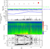 |
Fig. 2 PSP/RFS radio frequency data showing the type III bursts and storm on 2 April 2019. Top panel: normalised Stokes intensity above 18 MHz, second panel: full spectrogram, third panel: significant burst above the background, and bottom panel: frequency of maximum normalised intensity. This interval shows both more classical type III bursts and the weaker more localised features associated with type III radio storms. These data are described further in the text. |
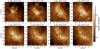 |
Fig. 3 Evolution of the active region from its emergence on 31 March to 7 April 2019. The active region has a simple structure, with expansion clearly seen, especially between 31 March and 3 April. |
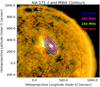 |
Fig. 4 AIA’s 171 Å solar image overlaid with the MWA radio contours at four frequency bands. The time corresponding to the AIA image is 04:01:45 UT. The contour levels corresponding to 164, 192, and 240 MHz are 50, 70, 80, and 90% with respect to the map’s maximum TB, respectively.The contour levels corresponding to the 108 MHz radio source are 70, 80, 90, and 99%, with respect to the map’s maximum TB. |
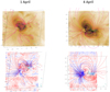 |
Fig. 5 Top two panels: magnetic field model of the active region on 1 April and 4 April overlaid on AIA 193 Å images with the intensity reversed. Bottom two panels: same model, but overlaid on the Doppler velocity maps with blue showing blue shifts and red showing red shifts (the colour range is +/−20 km s−1). The AR expands as it evolves. At its edges on 1 April, we observe structures in AIA data that are closed within theAR. On 4 April, the magnetic field lines derived from our model look more expanded at the edges of the AR, and larger scale magnetic field lines are relevant in correspondence with the blue-shifted region. The axes in all panels are labelled in Megametres, with the origin set in the AR centre (located at N12E31on 1 April and at N13W05 on 4 April). The iso-contours of the line-of-sight field correspond to ±50, ±100, and ±500 G in continuous magenta (blue) style for the positive (negative) values. Sets of computed field lines matching the global shape of theobserved coronal loops in the AIA 193 Å images were added in a continuous line and red colour in the two top panels and repeated in the two bottom panels. |
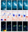 |
Fig. 6 Top panel: EIS Fe XII 195.119 Å intensity maps of the active region as it crossed the disc from 1 to 6 April. Centre panel: Doppler velocity maps derived from the same line. The colour bar shows the velocity range. The white boxes indicate the outflow regions chosen for measuring the FIP bias. Bottom panel: non-thermal velocity maps also from Fe XII 195.119 Å. |
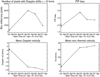 |
Fig. 7 Top left panel: number of pixels of the blue-shifted region as the active region crossed the disc from 1 to 6 April. The area of the blue-shifted region increases as the AR evolves. Top right panel: FIP bias measurements in the outflow area (white boxes in Fig. 6). The FIP bias appears to increase on 4 April when the blue-shifted area also reaches a maximum. Bottom left panel: variation of the mean of Doppler velocity in the same region. Bottom right panel: variation of mean of non-thermal velocity in the same region. Both the Doppler velocity and non-thermal velocity show a significant increase in magnitude in the first few days of the active region’s formation. |
4 High cadence observations from Hinode EIS and comparison to PSP data
From the foregoing discussion, it is clear that the blue-shifted region is the most likely source of the SEPs within the studied active region. In this section, we analyse a high cadence EIS dataset to search for dynamical behaviour, similar to that which is seen in the PSP data, during a one-hour period starting from 17:00UT on 1 April. The EIS data consisted of a series of fast rasters over a small field-of-view, each of which took 41 s to complete. As already noted, the type III storm consists of continuous small and frequency localised bursts, and these are repeating on timescales of minutes. This is another property that may help discriminate the source region.
In the right panel of Fig. 8, the EIS Doppler velocity in the blue-shifted region is shown above, and the PSP data are shown below for the one-hour time period. The Doppler velocities in this region show small but continuous variations and also on timescales of minutes. This is consistent with the nature of the type III bursts and also with the analysis carried out by Ugarte-Urra & Warren (2011). Ugarte-Urra & Warren (2011) also found that the blue-shifted outflow regions showed transient blue wing enhancements within the 5min cadence of their observations. The errors on the Hinode EIS Doppler velocity measurements are of the order of a few km s−1, which means these fluctuations are on the edge of detectability for these measurements.
We investigated the properties of the AR core to see if it could potentially be the source through small-scale brightenings. We analysed the variability of the AR core in AIA data during the same one-hour time period as the EIS high cadence scan. We already ruled out significant flaring during this time, but it is important to check for any small scale micro-flaring, so we produced a running difference movie to highlight any brightenings that occur in the core. We then extracted the number of brightenings which were definedas having an area >15 AIA pixels and have an intensity enhancement compared to the previous image of at least 100 DN. Figure 9 shows the light curve of the whole active region. The longer timescale changes that are seen over ≈ 30 min are due to the intensity increase of ‘new’ loops. The plot below shows when and how many brightenings occur in the core, and we find that they do not happen consistently during the whole hour period. We also searched in the XRT data for jets and found none. Hencewe infer that the fluctuations seen in the AR core are not viable as sources of the continuous type III bursts seen by PSP.
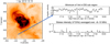 |
Fig. 8 Left panel: AIA 193 Å image with the field-of-view of the EIS fast scan overlaid. Within the EIS raster we chose a small regionof interest focused in the blue-shifted region. A blue arrow highlights this region of interest. Right panel, top: variation of the Doppler velocity during the one-hour raster. Bottom: variations in the PSP data and the frequency of the type III bursts for the same time interval. |
 |
Fig. 9 Top panel: lightcurve of the AIA intensity in the 193 AA filter. Bottom panel: number of brightenings in the AIA running difference movie that have a ‘blob’ size with an area more than 15 pixels and an intensity enhancement of > 100 DN. |
5 Conclusions
We have analysed the behaviour of AR 12737 during the time period of 31 March to 6 April 2019 around perihelion (4 April) of the second encounter of PSP. During this time, on a backdrop of larger, more impulsive type III bursts, PSP/FIELDS detected numerous small type III bursts constituting a radio noise storm. These type III bursts:
-
were rapid and persistent during the time interval;
-
exhibited a decreasing peak frequency indicating a source altitude which increases in time, or a source region which is becoming more rarefied with time; and
-
The behaviour of these type II bursts are consistent with an expanding source region becoming more open to the solar wind.
AR 12737 is the most probable candidate source region for this type III noise storm. It is seen to emerge near the east limb at the same time as the radio noise storm develops. Between 1 and 4 April, as the noise storm evolved as described above, this active region also showed the following significant changes:
-
the area of the blue-shifted outflow region increased by an order of magnitude;
-
the FIP bias increased in the blue-shifted region by a significant amount (consistent with an increase in SEPs; Reames 2018);
-
the whole active region expanded and, consequently, large-scale or expanding magnetic field lines anchored at the AR edge are more evident (including in the outflow region); and
-
the magnitude of the Doppler velocity and the non-thermal velocity increases significantly as the active region expands in its first few days of formation.
The behaviour and changes in the AR during this time period are consistent with the source of the type III bursts being the blue-shifted outflow region. We also explored the dynamics of the outflow region which do show fluctuations on the time scale of the cadence of the observations. However, these fluctuations are close to the measurement limit of the instrument, and they provide a tantalising hint of dynamics. The high cadence aspect of these measurements is key to further understanding the sources of SEPs and we encourage the future observing campaigns with PSP to aim to have some fast cadence measurements.
In addition, the expansion of the blue-shifted area of the active region may offer insight into the generation mechanism of type III storms. At least in this example, the decreasing peak frequency of the noise storm with time is suggestive of a scenario in which an expanding open field region allows the energetic electrons to more readily escape and thus produce their peak emission higher in the corona. Alternatively, the increasing open field region may allow more plasma to evacuate into interplanetary space, causing a rareification of the source region and hence a decreasing plasma frequency. The EIS composition measurements could be consistent with either scenario. Both an increase in escaping energetic particles and/or source plasma would lead to a greater fraction of the total emission in the outflow areas we measured being contributed by higher FIP bias plasma and, therefore, increasing the mean value. The decreasing trend in the FIP bias after the peak on 4 April is consistent with a decrease in the magnitude of the type III bursts.
Acknowledgements
We acknowledge support from ISSI for the team 463, entitled ‘Exploring The Solar Wind In Regions Closer ThanEver Observed Before’. The work of DHB was performed under contract to the Naval Research Laboratory and was funded by the NASA Hinode program. L.H. and K.B. are grateful for SNSF support (project number 200021_188390) C.H.M. acknowledges financial support from the Argentine grants PICT 2016-0221 (ANPCyT) and UBACyT 20020170100611BA (UBA). C.H.M. is a member of the Carrera del Investigador Científico of the Consejo Nacional de Investigaciones Científicas y Técnicas (CONICET). Hinode is a Japanese mission developed and launched by ISAS/ JAXA, with NAOJ as domestic partner and NASA and STFC (UK) as international partners. It is operated by these agencies in cooperation with ESA and NSC (Norway). This scientific work makes use of the Murchison Radio-astronomy Observatory (MRO), operated by the Commonwealth Scientific and Industrial Research Organisation (CSIRO). We acknowledge the Wajarri Yamatji people as the traditional owners of the Observatory site. Support for the operation of the MWA is provided by the Australian Government’s National Collaborative Research Infrastructure Strategy (NCRIS), under a contract to Curtin University administered by Astronomy Australia Limited. We acknowledge the Pawsey Supercomputing Centre, which is supported by the Western Australian and Australian Governments. The SDO data are courtesy of NASA/SDO and the AIA, EVE, and HMI science teams. CHIANTI is a collaborative project involving George Mason University, the University of Michigan (USA), University of Cambridge (UK) and NASA Goddard Space Flight Center (USA). The FIELDS instrument on the Parker Solar Probe spacecraft was designed and developed under NASA contract NNN06AA01C. Contributions from S.T.B. were supported by NASA Headquarters under the NASA Earth and Space Science Fellowship Program Grant 80NSSC18K1201. R.S. acknowledges support from the Swiss National Science foundation (grant no. 200021_175832). Contribution from K.B. were supported by Swiss National Science Foundation.
References
- Badman, S. T., Bale, S. D., Martínez Oliveros, J. C., et al. 2020, ApJS, 246, 23 [Google Scholar]
- Bale, S. D., Goetz, K., Harvey, P. R., et al. 2016, Space Sci. Rev., 204, 49 [Google Scholar]
- Bale, S. D., Badman, S. T., Bonnell, J. W., et al. 2019, Nature, 576, 237 [Google Scholar]
- Brooks, D. H., & Warren, H. P. 2011, ApJ, 727, L13 [Google Scholar]
- Brooks, D. H., & Warren, H. P. 2016, ApJ, 820, 63 [Google Scholar]
- Brooks, D. H., Ugarte-Urra, I., & Warren, H. P. 2015, Nat. Commun., 6, 5947 [Google Scholar]
- Brooks, D. H., Winebarger, A. R., Savage, S., et al. 2020, ApJ, 894, 144 [Google Scholar]
- Cattell, C., Glesener, L., Leiran, B., et al. 2021, A&A, 650, A6 (PSP SI) [EDP Sciences] [Google Scholar]
- Culhane, J. L., Harra, L. K., James, A. M., et al. 2007, Sol. Phys., 243, 19 [Google Scholar]
- Del Zanna, G. 2013, A&A, 555, A47 [NASA ADS] [CrossRef] [EDP Sciences] [Google Scholar]
- Del Zanna, G., Aulanier, G., Klein, K. L., & Török, T. 2011, A&A, 526, A137 [NASA ADS] [CrossRef] [EDP Sciences] [Google Scholar]
- Del Zanna, G., Dere, K. P., Young, P. R., Landi, E., & Mason, H. E. 2015, A&A, 582, A56 [NASA ADS] [CrossRef] [EDP Sciences] [Google Scholar]
- Démoulin, P., Bagalá, L. G., Mandrini, C. H., Hénoux, J. C., & Rovira, M. G. 1997, A&A, 325, 305 [Google Scholar]
- Dere, K. P., Landi, E., Mason, H. E., Monsignori Fossi, B. C., & Young, P. R. 1997, A&AS, 125, 149 [NASA ADS] [CrossRef] [EDP Sciences] [Google Scholar]
- Fox, N. J., Velli, M. C., Bale, S. D., et al. 2016, Space Sci. Rev., 204, 7 [NASA ADS] [CrossRef] [Google Scholar]
- Green, L. M., López fuentes, M. C., Mandrini, C. H., et al. 2002, Sol. Phys., 208, 43 [Google Scholar]
- Grevesse, N., Asplund, M., & Sauval, A. J. 2007, Space Sci. Rev., 130, 105 [Google Scholar]
- Harra, L. K., Sakao, T., Mandrini, C. H., et al. 2008, ApJ, 676, L147 [Google Scholar]
- Horbury, T. S., Woolley, T., Laker, R., et al. 2020, ApJS, 246, 45 [Google Scholar]
- Kamio, S., Hara, H., Watanabe, T., Fredvik, T., & Hansteen, V. H. 2010, Sol. Phys., 266, 209 [Google Scholar]
- Kashyap, V., & Drake, J. J. 1998, ApJ, 503, 450 [Google Scholar]
- Kashyap, V., & Drake, J. J. 2000, Bull. Astron. Soc. India, 28, 475 [NASA ADS] [EDP Sciences] [Google Scholar]
- Kasper, J. C., Bale, S. D., Belcher, J. W., et al. 2019, Nature, 576, 228 [Google Scholar]
- Krucker, S., Kontar, E. P., Christe, S., Glesener, L., & Lin, R. P. 2011, ApJ, 742, 82 [Google Scholar]
- Krupar, V., Szabo, A., Maksimovic, M., et al. 2020, ApJS, 246, 57 [Google Scholar]
- Leblanc, Y., Dulk, G. A., & Bougeret, J.-L. 1998, Sol. Phys., 183, 165 [NASA ADS] [CrossRef] [Google Scholar]
- Lonsdale, C. J., Cappallo, R. J., Morales, M. F., et al. 2009, IEEE Proc., 97, 1497 [Google Scholar]
- Mandrini, C. H., Baker, D., Démoulin, P., et al. 2015, ApJ, 809, 73 [Google Scholar]
- Mariska, J. T. 1994, ApJ, 434, 756 [Google Scholar]
- Mohan, A., & Oberoi, D. 2017, Sol. Phys., 292, 168 [Google Scholar]
- Morioka, A., Miyoshi, Y., Iwai, K., et al. 2015, ApJ, 808, 191 [Google Scholar]
- Mulay, S. M., Sharma, R., Valori, G., et al. 2019, A&A, 632, A108 [EDP Sciences] [Google Scholar]
- Pesnell, W. D., Thompson, B. J., & Chamberlin, P. C. 2012, Sol. Phys., 275, 3 [Google Scholar]
- Pulupa, M., Bale, S. D., Bonnell, J. W., et al. 2017, J. Geophys. Res. Space Phys., 122, 2836 [Google Scholar]
- Pulupa, M., Bale, S. D., Badman, S. T., et al. 2020, ApJS, 246, 49 [Google Scholar]
- Reames, D. V. 2017, Lect. Notes Phys. (Springer International Publishing AG), 932 [Google Scholar]
- Reames, D. V. 2018, Space. Sci. Rev., 214, 61 [Google Scholar]
- Reid, H. A. S., & Ratcliffe, H. 2014, Res. Astron. Astrophys., 14, 773 [Google Scholar]
- Sterling, A. C., & Moore, R. L. 2020, ApJ, 896, L18 [Google Scholar]
- Tingay, S. J., Goeke, R., Bowman, J. D., et al. 2013, PASA, 30, e007 [Google Scholar]
- Ugarte-Urra, I., & Warren, H. P. 2011, ApJ, 730, 37 [NASA ADS] [CrossRef] [Google Scholar]
- Wayth, R. B., Tingay, S. J., Trott, C. M., et al. 2018, PASA, 35, 33 [Google Scholar]
- Zlotnik, E. I. 1981, A&A, 101, 250 [Google Scholar]
All Figures
|
Fig. 1 PSP/RFS, RSTN, and MWA radio frequency measurements, AIA 193 Å intensity, and GOES X-ray data over the full interval from 30 March 2019 to 6 April 2019. Top panel: daily RSTN flux from 30 March to 6 April 2019 at 245 MHz. The red circle marks the flux at 240 MHz obtained from the MWA flux calibration, with error bars from the temporal RMS each day. Second panel: GOES soft X-ray flux data, which do not show any significant flares. Third panel: AIA 193 Å intensity integrated over the FOV shown in Fig. 3, showing the growth and flattening off of the development of the AR from 31 March to 4 April. Fourth panel: again the normalised Stokes intensity above 18 MHz and fifth panel: again the full spectrogram. Sixth panel: frequency of the peak normalised signal (as per Fig. 2). Bottom panel: inferred source height of the radio emission, inverting the peak frequency from a solar wind density profile and fundamental emission, as described in the text. The noise storm commenced on 31 March and a clear trend between 1 April to 4 April shows the peak type III storm emission frequency decreasing, corresponding to a higher source altitude or a more rarefied source region. |
| In the text | |
|
Fig. 2 PSP/RFS radio frequency data showing the type III bursts and storm on 2 April 2019. Top panel: normalised Stokes intensity above 18 MHz, second panel: full spectrogram, third panel: significant burst above the background, and bottom panel: frequency of maximum normalised intensity. This interval shows both more classical type III bursts and the weaker more localised features associated with type III radio storms. These data are described further in the text. |
| In the text | |
|
Fig. 3 Evolution of the active region from its emergence on 31 March to 7 April 2019. The active region has a simple structure, with expansion clearly seen, especially between 31 March and 3 April. |
| In the text | |
|
Fig. 4 AIA’s 171 Å solar image overlaid with the MWA radio contours at four frequency bands. The time corresponding to the AIA image is 04:01:45 UT. The contour levels corresponding to 164, 192, and 240 MHz are 50, 70, 80, and 90% with respect to the map’s maximum TB, respectively.The contour levels corresponding to the 108 MHz radio source are 70, 80, 90, and 99%, with respect to the map’s maximum TB. |
| In the text | |
|
Fig. 5 Top two panels: magnetic field model of the active region on 1 April and 4 April overlaid on AIA 193 Å images with the intensity reversed. Bottom two panels: same model, but overlaid on the Doppler velocity maps with blue showing blue shifts and red showing red shifts (the colour range is +/−20 km s−1). The AR expands as it evolves. At its edges on 1 April, we observe structures in AIA data that are closed within theAR. On 4 April, the magnetic field lines derived from our model look more expanded at the edges of the AR, and larger scale magnetic field lines are relevant in correspondence with the blue-shifted region. The axes in all panels are labelled in Megametres, with the origin set in the AR centre (located at N12E31on 1 April and at N13W05 on 4 April). The iso-contours of the line-of-sight field correspond to ±50, ±100, and ±500 G in continuous magenta (blue) style for the positive (negative) values. Sets of computed field lines matching the global shape of theobserved coronal loops in the AIA 193 Å images were added in a continuous line and red colour in the two top panels and repeated in the two bottom panels. |
| In the text | |
|
Fig. 6 Top panel: EIS Fe XII 195.119 Å intensity maps of the active region as it crossed the disc from 1 to 6 April. Centre panel: Doppler velocity maps derived from the same line. The colour bar shows the velocity range. The white boxes indicate the outflow regions chosen for measuring the FIP bias. Bottom panel: non-thermal velocity maps also from Fe XII 195.119 Å. |
| In the text | |
|
Fig. 7 Top left panel: number of pixels of the blue-shifted region as the active region crossed the disc from 1 to 6 April. The area of the blue-shifted region increases as the AR evolves. Top right panel: FIP bias measurements in the outflow area (white boxes in Fig. 6). The FIP bias appears to increase on 4 April when the blue-shifted area also reaches a maximum. Bottom left panel: variation of the mean of Doppler velocity in the same region. Bottom right panel: variation of mean of non-thermal velocity in the same region. Both the Doppler velocity and non-thermal velocity show a significant increase in magnitude in the first few days of the active region’s formation. |
| In the text | |
|
Fig. 8 Left panel: AIA 193 Å image with the field-of-view of the EIS fast scan overlaid. Within the EIS raster we chose a small regionof interest focused in the blue-shifted region. A blue arrow highlights this region of interest. Right panel, top: variation of the Doppler velocity during the one-hour raster. Bottom: variations in the PSP data and the frequency of the type III bursts for the same time interval. |
| In the text | |
|
Fig. 9 Top panel: lightcurve of the AIA intensity in the 193 AA filter. Bottom panel: number of brightenings in the AIA running difference movie that have a ‘blob’ size with an area more than 15 pixels and an intensity enhancement of > 100 DN. |
| In the text | |
Current usage metrics show cumulative count of Article Views (full-text article views including HTML views, PDF and ePub downloads, according to the available data) and Abstracts Views on Vision4Press platform.
Data correspond to usage on the plateform after 2015. The current usage metrics is available 48-96 hours after online publication and is updated daily on week days.
Initial download of the metrics may take a while.