| Issue |
A&A
Volume 650, June 2021
|
|
|---|---|---|
| Article Number | A139 | |
| Number of page(s) | 17 | |
| Section | Stellar structure and evolution | |
| DOI | https://doi.org/10.1051/0004-6361/202038126 | |
| Published online | 22 June 2021 | |
Measuring the masses and radii of neutron stars in low-mass X-ray binaries: Effects of the atmospheric composition and touchdown radius
1
Department of Physics, Ulsan National Institute of Science and Technology, Ulsan 44919, Korea
e-mail: myungkkim@unist.ac.kr; ymkim715@unist.ac.kr; kkwak@unist.ac.kr
2
Department of Physics, Pusan National University, Busan 46241, Korea
Received:
9
April
2020
Accepted:
26
March
2021
Context. X-ray bursts (XRBs) are energetic explosive events that have been observed in low-mass X-ray binaries (LMXBs). Some Type-I XRBs exhibit photospheric radius expansion (PRE) and these PRE XRBs are used to simultaneously estimate the mass and the radius of a neutron star in LMXB.
Aims. The mass and radius estimation depends on several model parameters, most of which are still uncertain. Here, we focus on the effects of the chemical composition of the photosphere, which determines the opacity during the PRE phase, and the touchdown radius, which can be larger than the neutron star radius. We investigate how these two model parameters affect the mass and radius estimation in a systematic way and whether there is any statistical trend for these two parameters as well as whether there is a possible correlation between them.
Methods. We used both a Monte Carlo (MC) sampling and a Bayesian analysis to examine the effects of the photospheric composition and the touchdown radius. We applied these two methods to six LMXBs exhibiting PRE XRBs. With both methods, we solved the Eddington flux equation and the apparent angular area equation, both of which include the correction terms. For the MC sampling, we developed an iterative method in order to solve these two equations more efficiently.
Results. We confirm that the effects of the photospheric composition and the touchdown radius are similar in the statistical and analytical estimation of mass and radius, even when the correction terms are considered. Furthermore, in all of the six sources, we find that a H-poor photosphere and a large touchdown radius are favored statistically regardless of the statistical method. Our Bayesian analysis also hints that touchdown can occur farther from the neutron star surface when the photosphere is more H-poor. This correlation could be qualitatively understood with the Eddington flux equation. We propose a physical explanation for this correlation between the photospheric composition and the touchdown radius. Our results show that when accounting for the uncertainties of the photospheric composition and the touchdown radius, it is most likely that the radii of the neutron stars in these six LMXBs are less than 12.5 km. This value is similar to that of the bounds placed on the neutron star radius based on the tidal deformability measured from the gravitational wave signal.
Key words: dense matter / opacity / stars: neutron / X-rays: binaries / X-rays: bursts
© ESO 2021
1. Introduction
Low-mass X-ray binaries (LMXBs) are the nesting systems in which thermonuclear (Type I) X-ray bursts (XRBs) are found. When a powerful XRB occurs, the maximum X-ray luminosity can reach the local Eddington limit (LEdd ∼ 1038 erg s−1) and it is possible for the photospheric layer to be lifted off the surface of the neutron star due to strong radiation pressure. When this happens, the photospheric radius can be much larger than the stellar radius of the neutron star. After the photospheric radius reaches its maximum, it returns to its original position, which is usually assumed to be the surface of the neutron star. This phenomenon is called photospheric radius expansion (PRE), with about 20% of all observed XRBs exhibiting the PRE feature (Galloway et al. 2008). Although the observed flux during the PRE stage is approximately constant because it is close to the local Eddington flux, it actually continues to increase, reaching a peak within a few seconds, and then decreases exponentially (Güver et al. 2010a). This happens because the temperature of the photosphere increases (decreases) while the size of the photosphere (i.e., photospheric radius) decreases (increases). At the moment that the observed flux reaches the peak, the temperature of the photosphere, which can be measured from the spectral analyses, reaches its maximum. Then the photospheric radius shrinks back to the minimum value, which is usually assumed to be the size of the neutron star. This moment is referred to as the “touchdown”.
Because the flux measured at the touchdown moment is still the local Eddington flux, it can be expressed as a function of mass and radius of the neutron star, the distance to the target, and the opacity of the photosphere. After the touchdown, the flux and the temperature continue to decrease and reach quasi-equilibrium, while the photospheric radius does not change. The flux and temperature measured at this later quasi-equilibrium phase provide the effective area of the observed X-ray emission, which is also a function of mass and radius of the neutron star and the distance to the target. Given two measured quantities, the touchdown flux and effective area, the mass and radius of the neutron star can be obtained simultaneously when additional observation information, such as the distance to the XRBs, is available. This approach has been suggested to estimate the mass and radius of the neutron star in the PRE XRBs and the first relatively accurate measurement was made for the neutron star in EXO 0748–6761 (Özel 2006).
We note that the above method is based upon the assumption that XRBs occur on the entire surface of the neutron star. There are a couple of theoretical and observational arguments that support this assumption. First, with a numerical model, Spitkovsky et al. (2002) proposed that the time scale of spreading the thermonuclear explosion on the entire surface of a rotating neutron star is considerably shorter (≪1 s) than that of the XRB itself, namely, from 10 to 100 s. The other argument is based upon the weak magnetic field of the neutron stars in LMXBs, which is supported by the observations, which do not detect strong pulsations in the steady state. If the magnetic field of the neutron star were strong, it would prevent the nuclear burning that causes XRBs from occurring on the entire surface of the neutron star. However, some uncertainties in the spectral analysis that contributes to the measurement of the effective area still remain. The observed blackbody spectrum often deviates from that of the true blackbody due to an atmospheric effect. If the emitting area were not perfectly spherical, the measurement of the effective area could also be altered. In order to address these uncertainties, a parameter called the “color-correction factor” is introduced in the equation for the effective area.
In paying further attention to the color-correction factor or the deviation from the blackbody spectrum during the cooling phase (i.e., after the touchdown), Suleimanov et al. (2011) suggested a new method called “cooling tail method”. In this approach, the spectral evolution during the cooling phase (which depends on the radiated flux – or the luminosity) is compared with the atmosphere model of a neutron star, which takes the surface gravity and chemical composition as input parameters. The comparison provides an alternative method for measuring the Eddington flux (and effective area), although the Eddington flux measured in this method was smaller than the measured touchdown flux for 4U 1724–307, which was analyzed as a test case. More recently, the cooling tail method was further developed into the “direct cooling tail method”, in which the direct comparison of the observed spectral evolution with the atmosphere model provides the mass and radius of the neutron star without inferring the Eddington flux and the effective area (Suleimanov et al. 2017). These authors applied the direct cooling tail method to SAX J1810.8–2609, which exhibits PRE, and compared the two (standard and direct cooling tail) methods. The direct cooling tail method was evolved further with the Bayesian approaches. By applying the Bayesian fitting between the model spectra predicted from the direct cooling tail model and the observed spectra from the five hard-state X-ray bursts of 4U 1702–429, Nättilä et al. (2017) derived the probable values for the mass and the radius of the neutron star in this LMXB, as well as the distance and the hydrogen mass fraction. Despite the success of the cooling tail method, however, the validity of the atmosphere model in application is limited. For example, by comparing the coherent oscillations observed during the quiescent phase to the XRB observations in 4U 1728–34, Zhang et al. (2016) found that the atmosphere model could only explain the observed spectrum during the cooling phase of a confined subset of XRBs that do not show oscillations during the quiescent phase.
When a powerful PRE XRB occurs, the temperature of the radiating region is high enough to fully ionize both H and He. As a result, the opacity of the photosphere is dominated by Thomson scattering and determined by the chemical composition of the photosphere, such as κ = 0.2(1 + X) cm2 g−1, where X is the hydrogen mass fraction in the H-He plasma. There have been both observational and theoretical efforts to constrain X. Observational efforts have been based upon the identification of the companion stars, including their stellar types, which could provide the information on the chemical composition of the accreted material. However, the chemical composition of the accreted material is not necessarily identical to that of the photosphere because of the steady-state burning of hydrogen into helium that takes place during accretion. Theoretical efforts, on the other hand, have been based upon the ignition model that explains how XRBs are empowered via the nuclear runaway reactions. According to this model, the ratio of the integrated persistent flux to the burst fluence can constrain the fuel type, that is, hydrogen, helium, and their mixture, since the burning of different types of fuel results in different levels of efficiency for energy production. Thus, the comparison of the observed ratio to the prediction could constrain the composition of the fuel, although the chemical composition of the fuel is neither necessarily identical to the photospheric composition. As a result, it remains uncertain whether it is possible to accurately constrain X, that is, the hydrogen mass fraction in the photosphere, which appears in the equations to determine the mass and radius of the neutron star in a LMXB, which shows PRE XRBs.
Since the first accurate measurement of Özel (2006), several LMXBs exhibiting PRE XRBs have been analyzed for the simultaneous estimation of the neutron star mass and radius with various methods, for example: (1) statistical methods to solve the Eddington flux equation and the apparent angular area equation, including the additional effects of spin and color temperature; and (2) the cooling tail method. A recent review is available in Özel & Freire (2016, along with the references therein). We note that different groups used different methods depending on their individual assumptions and the observational values they used. As a result, different values of mass and radius were obtained for the neutron stars even when based on identical PRE XRBs. However, most methods commonly dealt with two uncertain quantities, namely, the opacity and color correction factor, which are often considered as model-dependent parameters, although it is possible to constrain them observationally, in principle. Since the observational constraints on these quantities are not yet strong enough, previous works have been based upon statistical methods, such as a Monte Carlo (MC) sampling (also called a frequentist analysis) and a Bayesian analysis, which often adopts uniformly distributed values in the allowed range.
In this work, we take into account the possibility that touchdown occurs away from the neutron star surface, initially proposed by Steiner et al. (2010), and we revisit the estimation of the mass and radius of a neutron star in LMXB that shows PRE XRBs by focusing on the effects of the chemical composition of the photosphere and the touchdown radius. We investigate whether (or how much) the estimated mass and radius of the neutron star change systematically depending on the chemical composition of the photosphere and the touchdown radius. We also try to find whether there is any statistical trend for these two parameters, including any possible correlation between them. For our investigation, we use both a MC sampling and a Bayesian analysis and we apply these statistical methods to six LMXBs that had previously been analyzed either with the Bayesian method (e.g., Özel et al. 2016) or MC sampling (e.g., Steiner et al. 2010, with three targets).
In the next section, we describe the equations we used to estimate the mass and the radius of a neutron star in LMXB that shows PRE XRBs. In the same section, we also present the method of our MC sampling and Bayesian analysis. Our results and conclusions are presented in Sects. 3 and 4, respectively.
2. Method
2.1. Equations
We obtained two quantities, namely, touchdown flux (FTD, ∞) and apparent angular area (A), from the observed light curve and spectrum of PRE XRBs. These are expressed as functions of mass (M) and radius (R) of the neutron star, distance to the target (D), opacity (κ), and color-correction factor (fc) as in the following two equations, respectively:
where c, G, and σ are the speed of light, gravitational constant, and Stefan−Boltzmann constant, respectively. The  terms appear in order to include the effect of general relativity. FTD, ∞ and F∞ are measured from the light curve at the touchdown moment and at the later quasi-equilibrium phase after the touch down, respectively, and Tbb, ∞ is from the spectrum (at the later quasi-equilibrium phase). The ∞ subscript indicates that the quantities are measured from Earth.
In Eq. (1), touchdown is assumed to occur on the surface of the neutron star. This assumption was made by Özel (2006) who estimated the mass and radius of the neutron star in EXO 0748–676 relatively accurately for the first time. This assumption was also used for their later works, which estimated the masses and the radii of the neutron stars in other PRE XRBs (Güver et al. 2010a,b; Özel et al. 2009, 2010). However, Steiner et al. (2010) pointed out that this assumption resulted in poor acceptance rates in the MC simulations and suggested an alternative possibility that touchdown could occur away from the surface of the neutron star. In this assumption, R in Eq. (1) is replaced with rph, the photospheric radius, at which touchdown occurs, and Eq. (1) becomes
Subsequently, Özel et al. (2016) modified Eqs. (1) and (2) further by considering temperature correction on the touchdown flux and spin frequency (fNS) on the apparent angular area (A), as follows:
![$$ \begin{aligned} F_{\rm TD,\infty }&= {GMc \over {\kappa D^2}} \left(1 - {{2GM}\over {Rc^2}}\right)^{1/2} \nonumber \\&\left[1 + \left({kT_{\rm c} \over {38.8 \,\mathrm{keV}}}\right)^{a_g}\left(1 - {{2GM}\over {Rc^2}}\right)^{-a_g/2} \right]\!, \end{aligned} $$](/articles/aa/full_html/2021/06/aa38126-20/aa38126-20-eq5.gif)
where
and the color temperature (Tc) at touchdown is given as:
![$$ \begin{aligned} A&= f_{\rm c}^{-4}{R^2 \over {D^2}}\left(1 - {{2GM}\over {Rc^2}}\right)^{-1} \left\{ 1+\left[ \left(0.108 - 0.096 {M \over {M_{\odot }}}\right) \right. \right. \nonumber \\&\left. + \left(-0.061+0.114{M \over {M_{\odot }}}\right){R\over {10\mathrm{\,km}}} - 0.128\left({R\over {10\mathrm{\,km}}}\right)^2\right] \nonumber \\&\left. \left({f_{\rm NS} \over {1000\mathrm{\,Hz}}}\right)^2\right\} ^2. \end{aligned} $$](/articles/aa/full_html/2021/06/aa38126-20/aa38126-20-eq9.gif)
We note that touchdown is still occurring on the surface of the neutron star (rph = R) in Eq. (4).
In this work, we take into account the possibility that touchdown does not occur on the surface of the neutron star and apply it to Eq. (4). Then, Eqs. (4)–(7) for the touchdown flux can be re-written as follows, replacing R with rph.
![$$ \begin{aligned} F_{\rm TD,\infty }&= {GMc \over {\kappa D^2}} \left(1 - {{2GM}\over {{r_{\mathrm{ph} }}c^2}}\right)^{1/2} \nonumber \\&\left[1 + \left({kT_{\rm c} \over {38.8 \,\mathrm{keV}}}\right)^{a_g}\left(1 - {{2GM}\over {{r_{\mathrm{ph} }}c^2}}\right)^{-a_g/2} \right]\!, \end{aligned} $$](/articles/aa/full_html/2021/06/aa38126-20/aa38126-20-eq10.gif)
where
As in Steiner et al. (2010), we introduce the parameter, h, which determines the touchdown radius as a function of R, h = 2R/rph. We note that h has a value between 0 and 2, corresponding to rph = ∞ and rph = R, respectively. Equations (8) and (9) are solved for M and R when the values of touchdown flux (FTD, ∞), apparent angular area (A), distance to the target (D), opacity (κ), color-correction factor (fc), spin frequency (fNS), and h are given.
Although both fc and X, the two model-dependent parameters, are still uncertain, there have been theoretical and observational efforts to constrain them. We already mentioned the efforts to obtain X in the introduction. As for fc, Madej et al. (2004) suggested values ranging from 1.33 to 1.81 by considering the atmosphere models of a neutron star. This estimate is consistent with earlier calculations of London et al. (1986), Ebisuzaki & Nakamura (1988). As the flux approaches the local Eddington limit, fc increases but rarely exceeds 1.5 for a typical neutron star. However, in the tail of the bursts, fc approaches 1.33 due to a relatively low temperature (Madej et al. 2004). In this work, we adopt a range of fc between 1.33 and 1.47 for our MC sampling and between 1.35 and 1.45 for our Bayesian analysis (with the same central value of  ). We assume that fc is uniformly distributed within the range for both our MC sampling and Bayesian analysis. Two different ranges are taken from Özel et al. (2016) and Steiner et al. (2010), respectively, who also assumed that fc is uniformly distributed within the range. We believe that choosing a slightly different range for fc does not affect the conclusions of this paper.
2.2. Method 1: Monte Carlo sampling
In order to investigate the effects of the chemical composition of the photosphere (i.e., X) and the touchdown radius (i.e., h), we solved Eqs. (8) and (9) with fixed values of X and h (X = 0.1, 0.3, and 0.7 and h = 0, 1, and 2) while we take into account the distributions of the other variables based upon either observations or models. The exception for this is the spin frequency (fNS), which is given as a fixed value when its measurement is available, while a uniform distribution between 250 Hz and 650 Hz is used when it is not. By using the MC sampling, we generate independent values for FTD, ∞, A, D, and fc according to their distributions and we solve Eqs. (8) and (9) for mass and radius with these generated values and fixed values for X and h. The distributions of mass and radius are obtained as a result of the MC sampling. We can also get an acceptance rate, that is, the ratio of the number of physically possible solutions to the total number of the MC sampling.
In order to utilize the MC sampling method within a reasonable calculation time, it is necessary to solve Eqs. (8) and (9) relatively quickly. Since no analytic solution for M and R is found, we developed an iterative method that is faster than the full numerical methods. We note that Eq. (1) or Eq. (3) is solved for M and R analytically together with Eq. (2).
As the first step to solving Eqs. (8) and (9) for M and R, we call attention to the fact that the additional correction terms introduced by Özel et al. (2016) are not large (i.e., close to 1). Thus, Eqs. (8) and (9) can be re-written as:
where
![$$ \begin{aligned}&A_{\rm corr} = \left\{ 1+\left[ \left(0.108 - 0.096 {M \over {M_{\odot }}}\right) \right. \right. \nonumber \\&\qquad \left. + \left(-0.061+0.114{M \over {M_{\odot }}}\right){R\over {10\mathrm{\,km}}} - 0.128\left({R\over {10\mathrm{\,km}}}\right)^2\right] \nonumber \\&\qquad \, \left. \left({f_{\rm NS} \over {1000\mathrm{\,Hz}}}\right)^2\right\} ^2, \end{aligned} $$](/articles/aa/full_html/2021/06/aa38126-20/aa38126-20-eq18.gif)
Figure 1 confirms that the two correction terms are small unless a neutron star has an extremely small radius (large correction for the touchdown flux) or an extremely large radius with fast spin frequency (large correction for the apparent angular area). For a canonical value of M = 1.4 M⊙ and R = 10 km, the correction to the touchdown flux (with h = 2 which corresponds to rph = R) and the apparent angular area (with fNS = 600 Hz) is about 10% and 5%, respectively. In general, Fcorr decreases as h decreases, that is, when touchdown occurs farther away from the neutron star surface, although the mathematical limit of Fcorr does not converge to 1 exactly as h → 0. However, in the physical limit, Fcorr approaches 1 when h is sufficiently small because Fcorr comes from modification of opacity, due to the energy (temperature) dependence of scattering cross section, which becomes negligible when rph is sufficiently large. Suleimanov et al. (2012) mentioned the validity of the Fcorr formula, for example, Tc in the range of 2 to 50 keV, although they did not consider the case rph → ∞ (or very large). Below Tc = 2 keV, Fcorr approaches 1, that is, the modification of opacity becomes negligible. In Eq. (18), this can be achieved by setting Tc = 0 below 2 keV. Alternatively, we can treat Tc as a parameter that measures the effect of opacity modification by allowing it to decrease smoothly instead of being 0 abruptly below 2 keV. In this treatment, Tc can be smaller than 2 keV, depending on rph, meaning that Tc can trace the effect of opacity modification as a function of the touchdown radius. We tested how small h can be in order to treat Tc as a reasonable parameter and found that Fcorr behaves well with h = 10−2 to 10−3, which is good approximation for h ≈ 0. In the case of h = 0, therefore, we use FTD, ∞ = GMc/κD2 with Fcorr = 1.
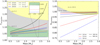 |
Fig. 1. Correction terms, Eqs. (16) and (18), are plotted as a function of mass for a range of radius which is indicated with different colors in both panels. For Fcorr (left panel), plots are drawn with three fixed values of h = 2R/rph. In the case of h = 0.01, all three lines are almost overlapping (see the inset). Acorr is not affected by h but by fNS, for which two values are selected (right panel). In both panels, regions for the causality limit (β = GM/Rc2 < 1/2.94) are indicated with different colors for different values of h and fNS. The regions above the boundaries are not allowed physically. |
In the next step, we utilize the analytic solutions for Eqs. (2) and (3), which are identical to Aorig and Forig, respectively. Following the procedures of Steiner et al. (2010), we define two new parameters α* and γ*,
The two parameters, α and γ, which were firstly defined and used in Steiner et al. (2010), specifically, in their Eqs. (16) and (17), are given as  and
and  , respectively, where
  . The analytic solutions (i.e., M and R) for Eqs. (2) and (3) are found by solving the α-equation for β for a given constant value of α and then by using the γ-equation for R with β obtained from the α-equation and a given constant value of γ (and M is obtained from β and R). The α-equation is generally a quartic equation for β with h, but for the two special cases that we are considering in this work, the α-equation becomes quadratic (h = 2) and cubic (h = 0) for β, respectively. Thus, we can write the α-equations for the three cases in our consideration which correspond to different fixed values of h (i.e., different touchdown radii), respectively, as follows.


The solution behaviors for Eqs. (21)–(23), such as constraints on the existence of physical solutions together with the causality limit (β < 1/2.94) were discussed in Steiner et al. (2010) who considered these behaviors and constraints in their MC sampling. For example, α < 3−3/2 ≈ 0.192, q2 + p3 < 0 [with  and
and  ], and α < 1/8 provide constraints for the existence of physically allowed solutions for Eqs. (21)–(23), respectively. Figure 2 shows two physically allowed solutions for the three α-equations, namely, Eqs. (21)–(23). We note that β± shown in Fig. 2 is obtained with the applied constraints on α.
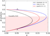 |
Fig. 2. Physically allowed solutions (β) for Eqs. (21)–(23) as a function of α. Solid lines represent β−, while dashed lines represent β+ ( β+ > β−). The red shade region indicates the causality limit (β < 1/2.94). Solutions within this region are physically meaningful. |
In our iterative method, we use the formal solutions of the α-equations, that is, Eqs. (21)–(23), the forms of which are known analytically, as in Steiner et al. (2010). Since  , the solution for Eq. (19) can be written as:

where f is the formal solution to Eqs. (21)–(23), that is, it corresponds to one of two β solutions for each α-equation. Similarly, with γ(M, R) = γ* Fcorr/Acorr,

From the previous step (Mn, Rn), we calculate βn = GMn/Rnc2 but it is not the same as f(α(Mn, Rn)) unless (Mn, Rn) is the solution. So, taking Δβ = f(α(Mn, Rn)) − βn, we update β as βn + 1 = f(α(Mn, Rn)). Similarly, if Rn is not the same as  , we update R as
  . The update of M is done as Mn + 1 = βn + 1Rn + 1c2/G. We repeat the same process with (Mn + 1, Rn + 1) until the following convergence condition is satisfied.


where we chose ε = 10−6. Due to the fact that the effects of the correction terms are not large (as we found in the first step), the convergence of this iterative method is fast when there is a solution. We checked out that our method solves Eqs. (19) and (20) for (M, R) correctly by plugging (M, R) back to the equations.
Since an iterative method is useful only for finding a solution that is known to exist within a range, it is necessary to address the existence of the solution separately. The existence of the solution is related to the condition for physically allowed solutions. Since the effects of the correction terms are not large, the solution behaviors for Eqs. (19) and (20) are not likely to deviate much from those for the α-equations, namely, Eqs. (21)–(23) (also see Fig. 2). Thus, it is reasonable to apply the same α-criteria of Eqs. (21)–(23) in order to constrain the existence of physically allowed solutions for Eqs. (19) and (20). In our iterative method, we set up a reasonably wide range of mass and radius, M = 1.5 ± 1.0 M⊙ and R = 15 ± 5 km, within which the initial guess for (M, R) is randomly selected. If the randomly selected (M, R) satisfies the α-criterion, we use this value of (M, R) as the initial guess of the iteration method. Otherwise, we move onto the next set of (M, R) which is also randomly generated within the same range of M and R. We conclude that there is no physically allowed solution when we do not find any α(M, R) that satisfies the α-criterion even if we search across a significantly large range of M and R with a significantly large (random) sampling number. We test and confirm the validity of our method to “identify unphysical solutions” by trying a wider range of mass and radius as well as by increasing the number of random sampling (nrs) for the case where there is no solution. For the results presented in this work, we use nrs = 1000 within the aforementioned range of M and R. We also confirm that the initial guess of (M, R) which satisfies the α-criterion always results in physically allowed solutions, which implies (or confirms self-consistently) that the effects of the correction terms are not large. We note that we apply the causality limit to the random sampling of (M, R), that is, the range of (M, R) is also limited with β < 1/2.94. For the entire scope of MC simulations, we carried out 106 realizations for each case (with three fixed values of X and h, respectively, for each source) to produce α* and γ*. For each case with the fixed value of X and h, the sampling is taken from the distributions of FTD, ∞, A, D, fNS, and fc. However, in the results which show the statistics for probable M and R, we exclude the events that do not have physically meaningful solutions from the statistical counting.
2.3. Method 2: Bayesian analysis
We also investigate the effects of the chemical composition and the touchdown radius by conducting a Bayesian analysis. Our calculation method is similar to that of the previous study in Özel et al. (2016) but we include a new model parameter, h, which determines the touchdown radius. Here, we briefly describe the Bayesian method we used. We refer to Özel et al. (2016) for more details of the Bayesian analysis used for the mass and radius estimation.
Our Bayesian analysis was done on two measured quantities: apparent angular size (A) and touchdown flux (FTD, ∞), with several model parameters: radius (R) and mass (M) of a neutron star, distance (D), spin frequency (fNS), color correction factor (fc), hydrogen mass fraction of the photosphere (X), and h for the touchdown radius (h = 2R/rph). From Bayes’ theorem, the posterior probability distribution P(θ|data) of the parameter set θ = {R, M, D, fNS, fc, X, h} on the given measured data (FTD, ∞, A) is expressed as:
where P(data|θ) is the likelihood and P(data) is the evidence. P(θ) is the prior of the parameter set θ of the model, which is composed of the multiplication of the prior distributions of the parameters as follows

We assume that the prior distributions of the radius and the mass of a neutron star, P(R) and P(M), are flat over given ranges, [2.0, 20.0] km and [0.65, 3.5] M⊙, respectively. The distance (D) to individual source is measured independently so that the prior distribution of the distance P(D) is a normal distribution taken from the measurement, except for EXO 1745–248 and KS 1731–260, for which a flat prior distribution is used (see Table 1). The prior distribution of the spin frequency of the neutron star P(fNS) is assumed to be flat between 250 Hz and 650 Hz if a measured fNS is not available. For a source that has a measured value of fNS, we chose P(fNS) as a delta function at the given value. We assume that P(fc) is flat over [1.35, 1.45]. Unlike our MC sampling, we do not fix X nor h for any source in our Bayesian analysis. Instead, we use flat prior distributions for these two model parameters and then obtain their posterior distributions, which we could use to investigate their effects. Furthermore, based upon the posterior distributions, we can investigate whether there exists any statistical trend for these two model parameters, including a possible correlation between them. The Bayesian approach is complementary to the MC sampling and provides a different approach for studying the effects of the chemical composition of the photosphere and the touchdown radius. We assume that P(X) and P(h) are flat over [0.0, 0.7] and [0.0, 2.0], respectively. The posterior distributions of the model parameters were obtained by carrying out the Markov-chain Monte Carlo (MCMC) simulations. We generated 2 × 10⁶ MCMC samples for each case under investigation based on the Metropolis-Hastings algorithm.
Observational properties of six LMXBs that show PRE XRBs.
3. Results
We applied our MC sampling and Bayesian analysis to six LMXBs exhibiting PRE XRBs. Table 1 presents the observed values with measurement uncertainties for these six sources. We chose and used the same observational values as in Özel et al. (2016), who analyzed these sources to estimate mass and radius by conducting a Bayesian analysis. But they did not consider the possibility that touchdown occurs at a larger radius than the neutron star radius. A subset of these six sources (three sources) were analyzed by Steiner et al. (2010), who investigated the effect of the touchdown radius by using the MC sampling. However, the latter authors did not consider the correction terms on the touchdown flux and the apparent angular size. We note that the observational values in Steiner et al. (2010) are slightly different from those in Table 1 – which are identical to those in Özel et al. (2016). Since the aim of the current work is to investigate the effects of the photospheric composition and the touchdown radius, we focus on the general trend that is commonly seen in six sources with varying X and h rather than on the results of individual sources. We refer to Steiner et al. (2010), Özel et al. (2016) for more details of individual sources, including general information on each source and the mass and radius estimations carried out with different methods.
3.1. Results from the MC sampling
The results obtained with the MC sampling (including our iterative method) for the six sources are shown in Tables 2–4 and Figs. 3–8. In Figs. 3–8, we also plotted the M − R curves predicted from nine EoS models. KIDS is a recently developed EoS model which is based upon density-functional theory. KIDS incorporates a perturbation scheme for the expansion of energy density-functional (Papakonstantinou et al. 2018). Both SGI and PAL6 take a potential-method approach (Li 1991; Prakash et al. 1988), but SGI is based upon the Skyrme force model more specifically. APR3 and ENG are a variational-method EoS and a relativistic Brueckner-Hartree-Fock EoS, respectively (Akmal et al. 1998; Engvik et al. 1996). All these five models include only regular nucleons, protons, and neutrons. However, H3 considers the hyperon contribution (Lackey et al. 2006) while SQM1,2,3 include the effect of quarks (Prakash et al. 1995). These two EoS models are based upon relativistic mean-field theory. We note that five EoS models in our selection (KIDS, SGI, APR3, ENG, and SQM2) can predict the neutron star mass larger than 2 M⊙, which is now a standard observational constraint (Demorest et al. 2010; Antoniadis et al. 2013). Tables 2–4 show the statistics of our MC sampling for the six sources. Out of 106 samples, the resulting events fall into one of three cases. The numbers in Tables 2–4 are the percentile of each case. The “solution” corresponds to the case that the physically allowed solution of mass and radius, either β− or β+, was found. Since one sampling for α* and γ* could result in two solutions (β±, see Fig. 2), we count each solution separately. Not all physically allowed solutions are true solutions due to the causality limit (β < 1/2.94). The “causality” corresponds to this case, that is, the events in the “solution” that violate the causality limit. As explained earlier in Sect. 2.2, the “unphysical” corresponds to the case that we can not find any physically meaningful solution by using the α-criterion. These unphysical solutions give non-real values of mass or radius. The M–R distributions in Figs. 3–8 are plotted only with the “solution” events. As a result, the distribution in each panel even within the same source is drawn from different number of events. In each panel, the maximum probability (indicated with red color) is calculated with the number of “solution” events in Tables 2–4 and the minimum probability (indicated with blue color) is chosen as 1/1000 of the maximum probability.
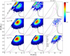 |
Fig. 3. Probability distributions of mass and radius obtained with our MC sampling for 4U 1820–30. Between two distance measurements for this source, we chose to use the larger one, namely, D = 8.4 ± 0.6 kpc, for the result shown here. In all panels, the 68% (solid white lines) and 95% (dot-dashed white lines) confidence contours are drawn. The color bar on the right reflects the relative probabilities the details of which are given in the text. The general relativistic causality limit (βlimit = 1/2.94) is drawn as a black straight line. From top to bottom: h = 2, h = 1 and h = 0, which correspond to rph = R (top), rph = 2R (middle), and rph ≫ R (bottom), respectively. From left to right: X = 0.1 (left), X = 0.3 (middle), and X = 0.7 (right). We note that the relative probabilities Pi of all distributions are normalized by ∫PidRdM = 1. For comparison, we also plot the mass–radius curves predicted from nine equation of state (EoS) models. See the text for the detailed description of these EoS models. |
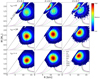 |
Fig. 4. Probability distributions of mass and radius obtained with our MC sampling for SAX J1748.9–2021. The description of the figure is the same as in Fig. 3. |
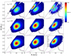 |
Fig. 5. Probability distributions of mass and radius obtained with our MC sampling for EXO 1745–248. The description of the figure is the same as in Fig. 3. |
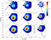 |
Fig. 6. Probability distributions of mass and radius obtained with our MC sampling for KS 1731–260. The description of the figure is the same as in Fig. 3. |
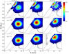 |
Fig. 7. Probability distributions of mass and radius obtained with our MC sampling for 4U 1724–207. The description of the figure is the same as in Fig. 3. |
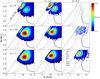 |
Fig. 8. Probability distributions of mass and radius obtained with our MC sampling for 4U 1608–52. The description of the figure is the same as in Fig. 3. |
Statistics of our MC sampling for six sources with rph = R (h = 2).
Statistics of our MC sampling for six sources with rph = 2R (h = 1).
Statistics of our MC sampling for six sources with rph ≫ R (h = 0).
Since we fix both X and h, the effect of each can be seen individually. The effect of X on the mass-radius estimation is seen as follows for all of the six sources. Regardless of h, as X increases, mass increases but radius decreases. It seems that this effect of X on mass and radius is not affected significantly by h. In other words, the change in the probability distributions of mass and radius (particularly the most probable values of mass and radius) with X appears to be similar for all three values of h. Comparably, the effect of h on the mass–radius estimation does not change much with X either. Regardless of X, as h decreases (i.e., touchdown occurs far from the neutron star surface), one of the two physically allowed solutions approaches close to and eventually crosses over the causality limit.
The effect of X on the mass–radius estimation can be explained based upon the equations given in Sect. 2.2. Since the effects of the correction terms are not large, that is, α* ≈ α and γ* ≈ γ. Then,  from Eq. (25) because αγ is now independent of X (or κ) from Eqs. (19) and (20), with their correction terms ignored. According to Eq. (19), α increases with X. Figure 2 shows how β± changes as a function of α. Since β− increases with α, R decreases with X. Since
  , M increases with X for the β− solution. However, on the contrary to β−, β+ decreases with α, which must result in the opposite trend, that is, the radius increases while the mass decreases with X. The correspondence of our results to the β+ solution seems to display this trend. For example, the most probable values of mass and radius obtained with h = 2 (i.e., rph = R) follow this trend (see the distributions close to the causality limit in the upper three panels in Figs. 3–8) although the trend does not appear clearly because the distributions are cut off at the causality limit. Another example may be found in the case of h = 1 (i.e., rph = 2R) in which the distributions corresponding to the β+ solution seem to appear for large X (see the distributions close to the causality limit in the middle three panels in Figs. 3–8) because the distributions for the β+ solution tend to move in the lower-right direction (↘) in the M–R space as X increases and can cross over the causality limit. However, in the case of h = 0 (i.e., rph ≫ R), we cannot see any distribution corresponding to the β+ solution because there is no physically allowed solution for β+ (see Fig. 2).
The explanation above is based upon the solution behaviors (as shown in Fig. 2) and it also applies when we are examining the effect of h. The distributions for mass and radius change with h simply because the value of h determines the behaviors of the β± solution. The distributions corresponding to the β+ solution are more likely to appear with a larger value of h, which corresponds to the case that touchdown occurs closer to the neutron star surface.
We ought to mention that the individual effect of X and h, which we find by fixing both, was already investigated in previous studies. In Steiner et al. (2010), who introduced h in their MC sampling analysis, the same effect of h on the mass-radius estimation was seen in their results although they did not consider the correction terms. But they did not investigate the effect of X because they did not vary X systematically. We note that among three sources that they analyzed, they fixed X = 0 for 4U 1820–30 when considering observational constraints on X for this source, but did not fix X for the other two sources (EXO 1745–248 and 4U 1608–52). The effect of X was tested for some individual sources which were previously analyzed with the probability transformation method. For example, for EXO 1745–248, Özel et al. (2009) found that X = 0 is favored after testing that X ≳ 0.1 does not result in any feasible solution with their method although they did not consider the correction terms to draw the conclusion for the effect of X. Thus, we believe that our results, which were obtained not only by including the correction terms and but also by using the MC sampling, can show the systematic effect of X (as well as of h) on the mass-radius estimation, although their effects can be inferred from the governing equations. Since we include the correction terms in our analysis, our results also confirm that the effects of the correction terms are not large enough to qualitatively change the effects of X and h. However, different values of fixed X and h result in different values of mass and radius. Figure 9 shows the estimated masses and radii that we obtained with fixed values of X and h in comparison with those in Özel et al. (2016). From Fig. 9, we can conclude that the upper limit of the most likely radii for these six sources is ∼12.5 km, regardless of the touchdown radius and the photospheric composition. We note that this upper bound is consistent with the bounds on the radii of neutron stars estimated from the tidal deformability of GW170817, measured by the LIGO and Virgo collaboration (Abbott et al. 2018).
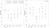 |
Fig. 9. Most probable values of mass (left panel) and radius (right panel) for the six sources that we obtained from our MC sampling for each of the values of X and h. The results from Özel et al. (2016) are also included for comparison. As in Fig. 3, we chose to use a larger distance only for 4U 1820–30. |
Although the way we treat X is different from that in Steiner et al. (2010), it is worth comparing how the acceptance rate (i.e., the percentiles of the physically allowed solutions in the results of the MC sampling) changes with the correction terms that are included for each run. For all of the common three sources (4U 1820–30, EXO 1745–248, and 4U 1608–52), we find that the acceptance rate increases as h decreases, which is consistent with what was found by Steiner et al. (2010). Again, this confirms that the correction terms do not significantly affect the overall solution behaviors of the governing equations that include the correction terms. We note that except for the h = 0 case of EXO 1745–248, X = 0.7 is strongly disfavored regardless of h for all the three sources. In fact, in all of the six sources, we find the same trend of the acceptance rate, such that the acceptance rate increases as h decreases. As for the acceptance rate as a function of X, which could not be addressed in Steiner et al. (2010), we find that for all of the six sources, the acceptance rate decreases as X increases. The trend of acceptance rate as a function of h and X is consistent with the results of our Bayesian analysis, presented in the next section.
3.2. Results from the Bayesian analysis
The results obtained with our Bayesian analysis are shown in Figs. 10–15. In these figures, we show the results only for four relevant model parameters, R, M, X, and h, among the total seven for which we obtained posterior distributions. We find that the posterior distributions of radius and mass for the six sources obtained from our Bayesian analysis are generally consistent with those from Özel et al. (2016). The shape of distribution and location of most probable value of (M, R) seems to be similar (but are not identical) in both results even if we include an additional model parameter h. From this comparison, one may conclude that the effect of h is not large in determining M and R in the Bayesian analysis. However, more detailed comparison based upon the posterior distributions of X and h reveal new findings. First of all, the hydrogen mass fraction is likely to be small in the posterior distributions for all of the six sources. In our Bayesian analysis, the prior distributions of X are uniform in [0, 0.7] in all of the six sources, but the posterior distributions of X are skewed to lower values and their medians are smaller than 0.35 (the mean of the prior distribution) in all of the six sources. The small values of X favored in the posterior distributions are consistent with the acceptance rate decreasing with X, which was found from our MC sampling. These results for X could imply that the photospheric composition is likely to be H-poor.
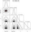 |
Fig. 10. Posterior distributions of neuron star mass (MNS) and radius (RNS), hydrogen mass fraction in the photosphere (X), and h = 2R/rph (which determines the touchdown radius) obtained from our Bayesian analysis for 4U 1820-30. In the panels that present the posterior distributions between two model parameters, the inner and outer solid line correspond to the 68% and 95% confidence contour, respectively. The most probable values of mass and radius are marked with red dots in the distribution plots of mass and radius. In the panels that present the posterior distribution of a single model parameter as a histogram, the region between two vertical dashed lines corresponds to the 68% confidence region. The numbers on top of the histogram panels present the corresponding 68% confidence range around the median value. Since there is no spin measurement available for 4U 1820-30, we use the prior distribution of fNS as a uniform distribution between 250 Hz and 650 Hz, which is the same as in Özel et al. (2016). |
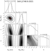 |
Fig. 11. Posterior distributions for SAX J1748.9-2021. The basic description of the figure is the same as in Fig. 10. For this source, fNS is available, so it was fixed at the measured value in Table 1. |
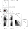 |
Fig. 12. Posterior distributions for EXO 1745–248. The basic description of the figure is the same as in Fig. 10. Since there is no spin measurement available for this source, we use the same prior distribution of fNS as in 4U 1820-30, i.e., a uniform distribution between 250 Hz and 650 Hz. |
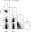 |
Fig. 13. Posterior distributions for KS 1731–260. The basic description of the figure is the same as in Fig. 10. For this source, fNS is available, so it was fixed at the measured value in Table 1. |
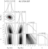 |
Fig. 14. Posterior distributions for 4U 1724–207. The basic description of the figure is the same as in Fig. 10. Since there is no spin measurement available for this source, we use the same prior distribution of fNS as in 4U 1820-30, i.e., a uniform distribution between 250 Hz and 650 Hz. |
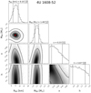 |
Fig. 15. Posterior distributions for 4U 1608–52. The basic description of the figure is the same as in Fig. 10. For this source, fNS is available, so it was fixed at the measured value in Table 1. |
We pay particular attention to 4U 1820–30 for which the posterior distribution of X is much smaller than those for the other sources. Small X for this target is consistent with the observational constraint on this source, namely, this target being an ultracompact binary with an H-poor donor (King & Watson 1986; Stella et al. 1987) and the theoretical constraint favoring H-poor fuel (Cumming 2003), both of which were already mentioned in Steiner et al. (2010). For this reason, both Steiner et al. (2010) and Özel et al. (2016) fixed X = 0 in their MC sampling and Bayesian analysis, respectively. We note that we chose a larger distance 8.4 ± 0.6 kpc for 4U 1820–30 in our Bayesian analysis between two available distance measurements in Table 1, while Özel et al. (2016) used both distance measurements by combining them as a double Gaussian distribution. The shape of the mass-radius distribution obtained from our analysis for 4U 1820–30 does not look very different from that in Özel et al. (2016), but our analysis has a larger value for most probable value of mass (M ≈ 1.99 M⊙ similar to the median) which may come from the choice of a different value for the distance. We note that among the six sources, 4U 1820–30 is the only source for which Özel et al. (2016) fixed X = 0.
Our analysis also reveals that h is not highly populated around 2.0 (which corresponds to the case of touchdown occurring on the neutron star surface) in the posterior distribution of h. We find this behavior of h in all of the six sources as well. The medians of h in all of the six sources are smaller than h = 1, corresponding to rph = 2R. In particular, as in the case of X, h favors smaller values for 4U 1820–30 than for the other sources. Our results for such behavior of h are consistent with the acceptance rate decreasing with h which was found from our MC sampling. These results on h could imply that touchdown is not likely to occur on the neutron star surface.
We also investigate the correlation between X and h based upon their posterior distributions by using the Pearson correlation test (Table 5). We find a relatively significant correlation between these two model parameters in five out of six sources for which |R|> 0.5. The correlation looks weak for 4U 1820–30 in which |R|< 0.5. Again, 4U 1820–30 shows an unusual feature in comparison with the other five sources. We note that the posterior distributions of both X and h for 4U 1820–30 are skewed more toward lower values. The (weak) anti-correlation between X and h could be explained based upon the equations in Sect. 2.2. By using, again, the fact that the effects of the correction terms are not significant, Eq. (3) leads to  , where we assume that M and β does not vary much with X and h. As X and h vary within a certain range while the assumption on M and β remains valid, we can expect the anti-correlation between them, namely, h increasing (decreasing) as X decreases (increases). However, this anti-correlation may not be as strong when the assumption on M and β breaks down or the solutions for mass and radius can be found only for small values of X or h – which might well be the case for 4U 1820–30.
Result of the Pearson correlation test between X and h over the posterior samples obtained within the 68% credible region.
We propose that the (weak) anti-correlation between X and h could be explained physically as well, given the relationship between the photospheric composition and the radiation pressure (which is determined by the Eddington flux as a function of the photospheric composition). If the photosphere is H-poor (i.e., small X), the radiation pressure decreases due to the small opacity with the same luminosity, which is determined by the thermonuclear reactions occurring below the photosphere. The decreased radiation pressure does not push the photosphere to a large distance so touchdown is also likely to occur close to the neutron star surface, that is, large h or h ≈ 2. In contrast, if the photosphere is H-rich, the photosphere can expand farther from the neutron star surface due to the large radiation pressure with large opacity and touchdown is likely to occur away from the neutron star surface. We note that this explanation for the weak anti-correlation between X and h is based upon the assumption that the fuel composition for thermonuclear burning, which determines the luminosity, is not correlated with the photospheric composition.
Finally, we point out that the most probable radii estimated with the Bayesian analysis, which includes the effects of both the touchdown radius and the photospheric composition, are less than 12.5 km, which is consistent with the results obtained with the MC sampling. This implies that the upper limit on the radii of the neutrons stars in six LMXBs analyzed in our study is valid, regardless of the statistical methods, when the uncertainties in the touchdown radius and the photospheric composition are taken into account.
4. Conclusion
In order to investigate the effects of the chemical composition of the photosphere and the touchdown radius on the estimation of mass and radius of a neutron star in LMXB that shows PRE XRB, we carried out statistical analyses on six LMXBs by using both a MC sampling and a Bayesian analysis. Following the approach of Steiner et al. (2010), we assume that touchdown occurs away from the neutron star surface and we introduce a new parameter, h, in our statistical analyses. For the six LMXBs we applied our MC sampling and Bayesian analysis to, we used the same observational data from Özel et al. (2016), who estimated the masses and radii of these six sources with their Bayesian analysis without h. In both methods, we solve the Eddington flux equation and the apparent angular area equation, both of which include the correction terms.
In our MC sampling, we fix both X (hydrogen mass fraction of the photosphere) and h at three values and investigate how the mass and radius estimation changes with these values of X and h. We confirm that the mass and the radius estimated with our MC sampling change with X and h as expected from the analytic solutions of the equations without correction terms. This result implies that the effects of the correction terms are not large enough to qualitatively change the effects of X and h, although different values of fixed X and h result in different values of mass and radius. We find that the acceptance rate, which is the ratio of the physically allowed solutions to the total realizations of our MC sampling, decreases with X and h in all of the six sources. This implies that small values of X and h are favored statistically, that is, the photosphere is likely to be H-poor regardless of the energy generation mechanism below the photosphere and that touchdown is likely to occur away from the neutron star surface. But we cannot conclude that there is any correlation between these two parameters based upon the MC sampling.
As a complementary analysis to the MC sampling, we chose flat prior distributions for both X and h in our Bayesian analysis instead of fixing them. We find that the posterior distributions of X and h are consistent with the acceptance rate decreasing with X and h, which was found from our MC sampling. In all of the six sources, the posterior distributions of X and h favor small values. By taking advantage of the Bayesian analysis, we investigated the correlation between X and h based upon the selected samples within the 68% confidence regions of the posterior distributions. We find that X and h are (weakly) anti-correlated in all of the six sources, which could be qualitatively understood with the Eddington flux equation. We propose that the anti-correlation between X and h could be explained physically as well, given the relationship between the radiation pressure and the opacity. Since the radiation pressure increases with opacity (or X) with the same luminosity on the photosphere, it is likely that touchdown occurs farther away from the neutron star surface (small h) after the strong radiation pressure (with large X) pushes the photosphere to a larger distance. Since we found this correlation in our analysis of six sources, it is worth investigating further whether the same correlation can be found for other LMXBs that show PRE XRBs.
We find that the upper bound of the most probable radii of the neutron stars in the six LMXBs analyzed with both the MC sampling and the Bayesian analysis in the current study, is around 12.5 km when the uncertainties on the touchdown radius and the photospheric composition are taken into account. It is interesting to note that this upper bound is similar to that placed by the LIGO and Virgo observations with the measurement of the tidal deformability of GW170817. Thus, it will be worth investigating whether a similar upper bound can be placed on the radii of neutron stars in other LMXBs.
Acknowledgments
We thank the referee for suggesting us to consider the effect of the touchdown radius together with that of the chemical composition of the photosphere. The referee’s suggestion and comments have greatly improved our earlier work. This work was supported by the National Research Foundation of Korea (NRF) grant funded by the Korea government (Ministry of Science and ICT) (No. 2016R1A5A1013277). MK and CHL were also supported by NRF grant funded by the Korea government (Ministry of Education) (No. 2018R1D1A1B07048599). YMK was also supported by NRF grants funded by the Korea government (MSIT) (No. 2019R1C1C1010571). KHS was also supported by NRF grant funded by Ministry of Education (NRF-2015H1A2A1031629-Global Ph.D. Fellowship Program). KK was also supported by NRF grant funded by Ministry of Education (No. 2016R1D1A1B03936169). We acknowledge the hospitality at the APCTP where part of this work was done. MK and YMK contributed equally to this work as co-first authors by carrying out the Monte Carlo sampling and the Bayesian analysis, respectively.
References
- Abbott, B. P., Abbott, R., Abbott, T. D., et al. (The LIGO Scientific Collaboration and the Virgo Collaboration) 2018, Phys. Rev. Lett., 121, 161101 [Google Scholar]
- Akmal, A., Pandharipande, V., & Ravenhall, D. 1998, Phys. Rev. C, 58, 1804 [NASA ADS] [CrossRef] [Google Scholar]
- Altamirano, D., Casella, P., Patruno, A., Wijnands, R., & van der Klis, M. 2008, ApJ, 674, L45 [NASA ADS] [CrossRef] [Google Scholar]
- Antoniadis, J., Freire, P. C. C., Wex, N., et al. 2013, Science, 340, 6131 [NASA ADS] [CrossRef] [PubMed] [Google Scholar]
- Cumming, A. 2003, ApJ, 595, 1077 [NASA ADS] [CrossRef] [Google Scholar]
- Demorest, P., Pennucci, T., Ransom, S., Roberts, M., & Hessels, J. 2010, Nature, 467, 1081 [NASA ADS] [CrossRef] [PubMed] [Google Scholar]
- Ebisuzaki, T., & Nakamura, N. 1988, ApJ, 328, 251 [NASA ADS] [CrossRef] [Google Scholar]
- Engvik, L., Bao, G., Hjorth-Jensen, M., Osnes, E., & Ostgaard, E. 1996, ApJ, 469, 794 [Google Scholar]
- Galloway, D. K., Muno, M. P., Hartman, J. M., et al. 2008, ApJS, 179, 360 [NASA ADS] [CrossRef] [Google Scholar]
- Güver, T., & Özel, F. 2013, ApJ, 765, L1 [Google Scholar]
- Güver, T., Özel, F., Cabrera-Lavers, A., & Wroblewski, P. 2010a, ApJ, 712, 964 [NASA ADS] [CrossRef] [Google Scholar]
- Güver, T., Wroblewski, P., Camarota, L., & Özel, F. 2010b, ApJ, 719, 1807 [Google Scholar]
- Hartman, J. M., Chakrabarty, D., Galloway, D. K., et al. 2003, BAAS, 35, 865 [Google Scholar]
- King, A. R., & Watson, M. G. 1986, Nature, 323, 105 [Google Scholar]
- Kuulkers, E., den Hartog, P. R., in ’t Zand, J. J. M., et al. 2003, A&A, 399, 663 [NASA ADS] [CrossRef] [EDP Sciences] [Google Scholar]
- Lackey, B. D., Nayyar, M., & Owen, B. J. 2006, Phys. Rev. D, 73, 024021 [CrossRef] [Google Scholar]
- Li, G.-Q. 1991, J. Phys. G, 17, 1 [Google Scholar]
- London, R. A., Taam, R. E., & Howard, W. M. 1986, ApJ, 306, 170 [Google Scholar]
- Madej, J., Joss, P. C., & Rożańska, A. 2004, ApJ, 602, 904 [NASA ADS] [CrossRef] [Google Scholar]
- Nättilä, J., Miller, M., Steiner, A., et al. 2017, A&A, 608, A31 [NASA ADS] [CrossRef] [EDP Sciences] [Google Scholar]
- Ortolani, S., Barbuy, B., Bica, E., Zoccali, M., & Renzini, A. 2007, A&A, 470, 1043 [NASA ADS] [CrossRef] [EDP Sciences] [Google Scholar]
- Özel, F. 2006, Nature, 441, 1115 [NASA ADS] [CrossRef] [PubMed] [Google Scholar]
- Özel, F., & Freire, P. 2016, ARA&A, 54, 401 [Google Scholar]
- Özel, F., Güver, T., & Psaltis, D. 2009, ApJ, 693, 1775 [Google Scholar]
- Özel, F., Baym, G., & Güver, T. 2010, Phys. Rev. D, 82, 101301 [Google Scholar]
- Özel, F., Gould, A., & Güver, T. 2012, ApJ, 748, 5 [Google Scholar]
- Özel, F., Psaltis, D., Güver, T., et al. 2016, ApJ, 820, 28 [NASA ADS] [CrossRef] [Google Scholar]
- Papakonstantinou, P., Park, T.-S., Lim, Y., & Hyun, C. H. 2018, Phys. Rev. C, 97, 014312 [Google Scholar]
- Prakash, M., Ainsworth, T. L., & Lattimer, J. M. 1988, Phys. Rev. Lett, 61, 2518 [Google Scholar]
- Prakash, M., Cooke, J., & Lattimer, J. 1995, Phys. Rev. D, 52, 661 [NASA ADS] [CrossRef] [Google Scholar]
- Smith, D. A., Morgan, E. H., & Bradt, H. 1997, ApJ, 479, L137 [NASA ADS] [CrossRef] [Google Scholar]
- Spitkovsky, A., Levin, Y., & Ushomirsky, G. 2002, ApJ, 566, 1018 [NASA ADS] [CrossRef] [Google Scholar]
- Steiner, A. W., Lattimer, J. M., & Brown, E. F. 2010, ApJ, 722, 33 [Google Scholar]
- Stella, L., White, N. E., & Priedhorsky, W. 1987, ApJ, 315, L49 [NASA ADS] [CrossRef] [Google Scholar]
- Suleimanov, V., Poutanen, J., Revnivtsev, M., & Werner, K. 2011, ApJ, 742, 122 [Google Scholar]
- Suleimanov, V., Poutanen, J., & Werner, K. 2012, A&A, 545, A120 [NASA ADS] [CrossRef] [EDP Sciences] [Google Scholar]
- Suleimanov, V. F., Poutanen, J., Nättilä, J., et al. 2017, MNRAS, 466, 906 [NASA ADS] [CrossRef] [Google Scholar]
- Valenti, E., Ferraro, F. R., & Origlia, L. 2007, AJ, 133, 1287 [NASA ADS] [CrossRef] [Google Scholar]
- Zhang, G., Mendez, M., Zamfir, M., & Cumming, A. 2016, MNRAS, 455, 2004 [NASA ADS] [CrossRef] [Google Scholar]
All Tables
Result of the Pearson correlation test between X and h over the posterior samples obtained within the 68% credible region.
All Figures
|
Fig. 1. Correction terms, Eqs. (16) and (18), are plotted as a function of mass for a range of radius which is indicated with different colors in both panels. For Fcorr (left panel), plots are drawn with three fixed values of h = 2R/rph. In the case of h = 0.01, all three lines are almost overlapping (see the inset). Acorr is not affected by h but by fNS, for which two values are selected (right panel). In both panels, regions for the causality limit (β = GM/Rc2 < 1/2.94) are indicated with different colors for different values of h and fNS. The regions above the boundaries are not allowed physically. |
| In the text | |
|
Fig. 2. Physically allowed solutions (β) for Eqs. (21)–(23) as a function of α. Solid lines represent β−, while dashed lines represent β+ ( β+ > β−). The red shade region indicates the causality limit (β < 1/2.94). Solutions within this region are physically meaningful. |
| In the text | |
|
Fig. 3. Probability distributions of mass and radius obtained with our MC sampling for 4U 1820–30. Between two distance measurements for this source, we chose to use the larger one, namely, D = 8.4 ± 0.6 kpc, for the result shown here. In all panels, the 68% (solid white lines) and 95% (dot-dashed white lines) confidence contours are drawn. The color bar on the right reflects the relative probabilities the details of which are given in the text. The general relativistic causality limit (βlimit = 1/2.94) is drawn as a black straight line. From top to bottom: h = 2, h = 1 and h = 0, which correspond to rph = R (top), rph = 2R (middle), and rph ≫ R (bottom), respectively. From left to right: X = 0.1 (left), X = 0.3 (middle), and X = 0.7 (right). We note that the relative probabilities Pi of all distributions are normalized by ∫PidRdM = 1. For comparison, we also plot the mass–radius curves predicted from nine equation of state (EoS) models. See the text for the detailed description of these EoS models. |
| In the text | |
|
Fig. 4. Probability distributions of mass and radius obtained with our MC sampling for SAX J1748.9–2021. The description of the figure is the same as in Fig. 3. |
| In the text | |
|
Fig. 5. Probability distributions of mass and radius obtained with our MC sampling for EXO 1745–248. The description of the figure is the same as in Fig. 3. |
| In the text | |
|
Fig. 6. Probability distributions of mass and radius obtained with our MC sampling for KS 1731–260. The description of the figure is the same as in Fig. 3. |
| In the text | |
|
Fig. 7. Probability distributions of mass and radius obtained with our MC sampling for 4U 1724–207. The description of the figure is the same as in Fig. 3. |
| In the text | |
|
Fig. 8. Probability distributions of mass and radius obtained with our MC sampling for 4U 1608–52. The description of the figure is the same as in Fig. 3. |
| In the text | |
|
Fig. 9. Most probable values of mass (left panel) and radius (right panel) for the six sources that we obtained from our MC sampling for each of the values of X and h. The results from Özel et al. (2016) are also included for comparison. As in Fig. 3, we chose to use a larger distance only for 4U 1820–30. |
| In the text | |
|
Fig. 10. Posterior distributions of neuron star mass (MNS) and radius (RNS), hydrogen mass fraction in the photosphere (X), and h = 2R/rph (which determines the touchdown radius) obtained from our Bayesian analysis for 4U 1820-30. In the panels that present the posterior distributions between two model parameters, the inner and outer solid line correspond to the 68% and 95% confidence contour, respectively. The most probable values of mass and radius are marked with red dots in the distribution plots of mass and radius. In the panels that present the posterior distribution of a single model parameter as a histogram, the region between two vertical dashed lines corresponds to the 68% confidence region. The numbers on top of the histogram panels present the corresponding 68% confidence range around the median value. Since there is no spin measurement available for 4U 1820-30, we use the prior distribution of fNS as a uniform distribution between 250 Hz and 650 Hz, which is the same as in Özel et al. (2016). |
| In the text | |
|
Fig. 11. Posterior distributions for SAX J1748.9-2021. The basic description of the figure is the same as in Fig. 10. For this source, fNS is available, so it was fixed at the measured value in Table 1. |
| In the text | |
|
Fig. 12. Posterior distributions for EXO 1745–248. The basic description of the figure is the same as in Fig. 10. Since there is no spin measurement available for this source, we use the same prior distribution of fNS as in 4U 1820-30, i.e., a uniform distribution between 250 Hz and 650 Hz. |
| In the text | |
|
Fig. 13. Posterior distributions for KS 1731–260. The basic description of the figure is the same as in Fig. 10. For this source, fNS is available, so it was fixed at the measured value in Table 1. |
| In the text | |
|
Fig. 14. Posterior distributions for 4U 1724–207. The basic description of the figure is the same as in Fig. 10. Since there is no spin measurement available for this source, we use the same prior distribution of fNS as in 4U 1820-30, i.e., a uniform distribution between 250 Hz and 650 Hz. |
| In the text | |
|
Fig. 15. Posterior distributions for 4U 1608–52. The basic description of the figure is the same as in Fig. 10. For this source, fNS is available, so it was fixed at the measured value in Table 1. |
| In the text | |
Current usage metrics show cumulative count of Article Views (full-text article views including HTML views, PDF and ePub downloads, according to the available data) and Abstracts Views on Vision4Press platform.
Data correspond to usage on the plateform after 2015. The current usage metrics is available 48-96 hours after online publication and is updated daily on week days.
Initial download of the metrics may take a while.