| Issue |
A&A
Volume 649, May 2021
|
|
|---|---|---|
| Article Number | A109 | |
| Number of page(s) | 17 | |
| Section | Stellar structure and evolution | |
| DOI | https://doi.org/10.1051/0004-6361/202140571 | |
| Published online | 26 May 2021 | |
The surface brightness–colour relations based on eclipsing binary stars and calibrated with Gaia EDR3⋆
1
Centrum Astronomiczne im. Mikołaja Kopernika, Polish Academy of Sciences, Rabiańska 8, 87-100 Toruń, Poland
2
Centrum Astronomiczne im. Mikołaja Kopernika, Polish Academy of Sciences, Bartycka 18, 00-716 Warsaw, Poland
3
Departamento de Astronomía, Universidad de Concepción, Casilla 160-C, Concepción, Chile
e-mail: darek@astro-udec.cl
4
Instituut voor Sterrenkunde, KU Leuven, Celestijnenlaan 200D, 3001 Leuven, Belgium
5
European Southern Observatory, Karl-Schwarzschild-Str. 2, 85748 Garching b. München, Germany
6
Université Côte d’Azur, Observatoire de la Côte d’Azur, CNRS, Laboratoire Lagrange, Nice, France
7
LESIA, Observatoire de Paris, Université PSL, CNRS, Sorbonne Université, Université de Paris, 5 place Jules Janssen, 92195 Meudon, France
8
Astrophysics Group, Keele University, Staffordshire ST5 5BG, UK
9
Department of Physics, University of Zagreb, Bijenićka cesta 32, 10000 Zagreb, Croatia
10
Leibniz-Institut für Astrophysik Potsdam, An der Sternwarte 16, 14482 Potsdam, Germany
11
Institute of Physics, Laboratory of Astrophysics, Ecole Polytechnique Fédérale de Lausanne (EPFL), Observatoire de Sauverny, 1290 Versoix, Switzerland
12
Unidad Mixta International Franco-Chilena de Astronomía (CNRS UMI 3386), Departamento de Astronomía, Universidad de Chile, Camino El Observatorio 1515, Las Condes, Santiago, Chile
13
LunAres Research Station, Airport, Hangar 11, Piła, Poland
Received:
15
February
2021
Accepted:
2
March
2021
Aims. The surface brightness–colour relation (SBCR) is a basic tool for establishing precise and accurate distances within the Local Group. Detached eclipsing binary stars with accurately determined radii and trigonometric parallaxes allow calibration of the SBCRs with unprecedented accuracy.
Methods. We analysed four nearby eclipsing binary stars containing late F-type main sequence components: AL Ari, AL Dor, FM Leo, and BN Scl. We determined very precise spectroscopic orbits and combined them with high-precision ground- and space-based photometry. We derived the astrophysical parameters of their components with mean errors of 0.1% for mass and 0.4% for radius. We combined those four systems with another 24 nearby eclipsing binaries with accurately known radii from the literature for which Gaia EDR3 parallaxes are available in order to derive the SBCRs.
Results. The resulting SBCRs cover stellar spectral types from B9 V to G7 V. For calibrations, we used Johnson optical B and V, Gaia GBP and G, and 2MASS JHK bands. The most precise relations are calibrated using the infrared K band and allow angular diameters of A-, F-, and G-type dwarf and subgiant stars to be predicted with a precision of 1%.
Key words: parallaxes / binaries: eclipsing / stars: distances
Full Tables 2 and 3 are only available at the CDS via anonymous ftp to cdsarc.u-strasbg.fr (130.79.128.5) or via http://cdsarc.u-strasbg.fr/viz-bin/cat/J/A+A/649/A109
© ESO 2021
1. Introduction
The concept of the stellar surface brightness parameter S is useful in astrophysics because it connects the stellar absolute magnitude M with the stellar radius R by a very simple relation (Wesselink 1969). It is very convenient to express the S parameter as a function of an intrinsic stellar colour, that is, the surface brightness–colour relation (SBCR), which is a powerful tool for predicting the angular diameters of stars (e.g., Barnes et al. 1976; Van Belle 1999; Kervella et al. 2004). When the distance (or the trigonometric parallax) to a particular star is known, application of an SBCR immediately gives its radius (Lacy 1977a). When, on the other hand, the radius of a star is known, an application of SBCR gives a robust distance (Lacy 1977b). The latter approach, in particular, has resulted in very precise distance determinations to the Magellanic Clouds (e.g., Pietrzyński et al. 2019; Graczyk et al. 2020), setting the zero-point of the extragalactic distance ladder with a precision of ∼1%.
In this paper we present a calibration of SBCRs based on eclipsing binary stars with trigonometric parallaxes. The fundamentals of the method are given in Graczyk et al. (2017). The first application of the method was presented by Stebbins (1910) in the case of Algol, but for many years a lack of parallaxes of sufficient quality for nearby eclipsing binaries has compromised a successful calibration of SBCRs this way. The results of the HIPPARCOS space mission (Perryman et al. 1997) showed that there are many nearby (d < 200 pc) eclipsing binaries suitable for the SBCR calibration. The best systems are those with well-detached, spotless components of similar temperature and size, and with a low interstellar reddening. Kruszewski & Semeniuk (1999) published a list of potential targets and during subsequent years we obtained photometric and spectroscopic follow-up data for about 50 eclipsing binaries based mostly on their list. The analysis of the HIPPARCOS sample proved to be difficult: many of the systems turned out to be multiple stars or active systems not suitable for the SBCR calibration, and photometric follow-up of sufficiently high quality was tedious and many parallaxes were of low precision. As a result we have so far published a full analysis of only two eclipsing binaries: IO Aqr (Graczyk et al. 2015) and LL Aqr (Graczyk et al. 2016). Also, for a few systems we derived the orbital parallaxes and precise masses but we assumed radii from the literature (Gallenne et al. 2016, 2019). However, with the advent of the space missions Gaia (Gaia Collaboration 2016), Kepler (Koch et al. 2010), and TESS (Ricker et al. 2015), the situation has improved dramatically. Here we present an analysis of four eclipsing binary stars and use Gaia parallaxes to obtain a very precise SBCR calibration.
2. Observations
2.1. Sample of stars
AL Ari, AL Dor, FM Leo, and BN Scl were discovered as variable stars during the HIPPARCOS space mission (Perryman et al. 1997), classified as eclipsing binaries and given names in the General Catalogue of Variable Stars (GCVS) by Kazarovets et al. (1999). Because the systems are well-detached, close to the Sun, and have no significant spot activity, we included them in our HIPPARCOS sample.
AL Ari was selected as a follow-up target in a photometric and spectroscopic survey of solar-type eclipsing binaries by Clausen et al. (2001). The preliminary physical parameters of this system were included in a compilation of eclipsing binaries prepared by Graczyk et al. (2017). AL Dor was included in a sample of eclipsing binaries used by Graczyk et al. (2019) to investigate the zero-point of the Gaia parallaxes. Precise masses of its components and an interferometric orbital parallax were derived by Gallenne et al. (2019). Here we present the full analysis of those two systems with updated physical parameters. An analysis of light- and radial velocity curves of FM Leo was published by Ratajczak et al. (2010), who derived the fundamental physical parameters of the system. Updated mass measurements of the components, together with the analysis of the Rossiter-McLaughlin effect, were provided by Sybilski et al. (2018). The last of the systems, BN Scl, has not yet been studied in detail. General data for the four systems are given in Table 1.
Basic data on the eclipsing binary stars.
2.2. Photometry
2.2.1. Ground-based Strömgren photometry
We used Strömgren uvby photometry of AL Ari secured with the Strömgren Automated Telescope (SAT) at ESO, La Silla (Clausen et al. 2001). The photometry was kindly provided to us by E. Olsen. The data were taken between October 1997 and December 1998 and comprise 827 differential magnitudes with respect to three comparison stars (HD 15814, 16707 and 17499) in each filter. The photometry was detrended and normalised separately in each filter; see Table 2.
uvby photometry of AL Ari.
2.2.2. Space-based photometry
AL Dor was observed by the TESS space mission (Ricker et al. 2015) in short cadence during sectors 1–13 and 27–29. We downloaded a total of 248 078 photometric data points collected by TESS from the Mikulski Archive for Space Telescopes (MAST) archive. The sectors differ somewhat in the number of artefacts and outliers, instrumental drifts, and observational noise. We decided to use only sectors 1–3, 12, and 27 in our analysis, as they have the smallest drifts and out-of-eclipse rms and cover a long time interval. Depending on the number of outliers and artefacts we used the Simple Aperture Photometry (SAPFLUX) or the Pre-search Data Conditioning SAP (PDCSAPFLUX) fluxes. The eclipse depths differ slightly between sectors, by up to 0.5% in flux. Only in the first five sectors is the depth constant to within 0.1%, and we renormalised the light curves from sectors 12 and 27 to reach the same minima depths. We retained all data during and close to eclipses, but kept only every fiftieth datapoint from the out-of-eclipse parts of the light curve. In total we used 6387 data points in our analysis below.
FM Leo was observed by the K2 mission (Howell et al. 2014), the extension of the Kepler space mission (Koch et al. 2010). It was observed during campaign 1 in 2014 in both long and short cadence. We downloaded these data from the MAST archive, containing 3192 long-cadence and 53 048 short-cadence datapoints. The data were detrended with a third-order spline function to remove only long-term flux changes and to keep the small ellipsoidal out-of-eclipse variations. The data were cleaned of obvious outliers and the fluxes were subsequently normalised. In order to lower the number of datapoints we removed short-cadence data taken outside eclipse and replaced them with the long-cadence data. This resulted in 6433 photometric points: 3756 short-cadence points around eclipses and 2677 long-cadence points outside eclipses.
BN Scl was observed by TESS in sectors 1 and 29. In both sectors some spot activity on the components can be noted, especially in the first part of the light curve from sector 1. The out-of-eclipse flux changes due to the spots are smaller than 0.5%, but they do slightly affect the shape and depth of the minima. From sector 29 we chose the data obtained in the time interval between BJD 2459088 and 2459100, when the light curve is most symmetric around both eclipses, that is, the fluxes were minimally influenced by the spots. We used the PDCSAPFLUX fluxes and retained points around eclipses and every second point in the out-of-eclipse parts of the light curve. In total we ended up with 3521 datapoints.
2.3. Spectroscopy
2.3.1. HARPS
We obtained spectra of the four systems with the High Accuracy Radial velocity Planet Searcher (HARPS; Mayor et al. 2003) on the European Southern Observatory 3.6-m telescope in La Silla, Chile. In total we collected 64 spectra between 2009 February 26 and 2015 June 21. The targets are bright and typical integration times were shorter than 10 min. The average signal-to-noise ratio (S/N) of the spectra was 75 for AL Dor, FM Leo and BN Scl, and 40 for AL Ari. All spectra were reduced on-site using the HARPS Data Reduction Software (DRS).
2.3.2. CORALIE
Thirty spectra were obtained for BN Scl and AL Dor with the CORALIE spectrograph on the Swiss 1.2-m Euler Telescope at La Silla between 2008 October 2 and 2010 November 1. The exposure times were between 800 s and 1100 s for BN Scl while for AL Dor they were between 520 s and 1100 s depending on the sky conditions and the airmass. A typical S/N near 5500 Å was 20 per pixel. The spectra taken during 2009 and 2010 were secured with a simultaneous ThAr lamp exposure, allowing us to correct for the intra-night radial-velocity drifts, while this was not possible for spectra taken during 2008; this may add some scatter to the radial velocities derived from CORALIE 2008 spectra. The spectra were reduced using the Geneva pipeline, which does all the standard steps.
3. Analysis of spectra
3.1. Radial velocities
We used the RaveSpan code (Pilecki et al. 2017) to measure the radial velocities of the components in all four systems via the Broadening Function (BF) formalism (Rucinski 1992, 1999). We used templates from the library of synthetic local thermodynamical equilibrium (LTE) spectra by Coelho et al. (2005) matching the mean values of estimated effective temperature and gravity of the stars in the binary. The abundances were assumed to be solar. The line profiles of the components of AL Ari, AL Dor, and FM Leo are Gaussian and suggest small rotational velocities, while the line profiles of the components of BN Scl are clearly rotationally broadened. The typical precision of radial velocity determination was about 20–30 m s−1 for AL Dor and FM Leo and about 50–100 m s−1 for the faster-rotating AL Ari and BN Scl. With RaveSpan we made initial radial-velocity solutions to the data and noted a small systematic drift in the O − C radial-velocity residuals of AL Ari (see Fig. 1). We fitted a linear function to the observed residuals and derived a radial-velocity acceleration of the AL Ari barycentre of 0.21 ± 0.04 m s−1 per orbital period (cycle). The trend was removed before we made full simultaneous light- and radial-velocity curve analysis of AL Ari. The radial-velocity measurements are summarised in Table 3.
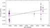 |
Fig. 1. Barycentric radial-velocity trend in AL Ari. The continuous line is a simple linear function fit to the trend. |
Radial-velocity measurements for eclipsing binary stars.
3.2. Spectra disentangling
We disentangled the observed composite spectra into those of the individual components of the binaries using an iterative method outlined by González & Levato (2006) and implemented in the RaveSpan code. This was done only for the HARPS spectra due to their higher S/N. We used the radial velocities previously measured and iterated twice. In order to account for the light contribution to the system from each star we renormalised the spectra using the photometric parameters from our simultaneous light- and radial-velocity curve solutions (see Sect. 5). The resulting individual spectra have S/N values at 5500 Å of about 100, except from the secondary component of AL Ari which has S/N = 40.
3.3. Stellar atmospheric analysis
3.3.1. Methods
We used the high-resolution disentangled HARPS spectra to derive the atmospheric parameters of the components of the binary systems. For this we employed the ‘Grid Search in Stellar Parameters’ (GSSP) software package designed for the analysis of high-resolution spectra of single stars and binary systems (Tkachenko 2015). We used the latest version of GSSP which makes use of the most recent (August 2020) version of the radiative transfer code, including a better solver for molecular transitions and improved calculation of the continuum, as well as a new, updated grid of atmosphere models. The code uses the spectrum synthesis method by employing the S YNTHV LTE-based radiative transfer code (Tsymbal 1996). We used a grid of atmosphere models that were calculated using the LL MODELS code (Shulyak et al. 2004). Important advantages of GSSP include its ability to perform fast calculations for large grids of synthetic models through the use of parallel computing via the O PENMPI implementation1 and an accurate treatment of limb darkening by computing the specific line and continuum intensities for different positions on the stellar disc.
Our approach relies on the use of the single and binary versions of the code. We aim to determine the surface atmospheric parameters such as the effective temperature (Teff), the surface gravity (log g), the metallicity ([M/H]), and the microturbulent velocity (ξ). More detailed investigation of surface abundances of individual chemical elements are scheduled for a follow-up paper. The GSSP_single module is designed for the analysis of the spectra of single stars or the disentangled spectra of the individual components of double-lined spectroscopic binary systems. To use this option the disentangled spectra should be renormalised appropriately, taking into account the wavelength dependence of the light dilution factor (fi). Otherwise, as the single version uses only the wavelength-independent fi, the results will be distorted the more the components of the system differ in Teff.
The GSSP_binary module is designed for dealing simultaneously with disentangled spectra of both components by taking into account the wavelength dependence of fi, which is defined as the fractional contribution of the individual components to the total light of the entire system (see Tkachenko 2015, for details). For our purposes, we used the ‘fit’ option to search for the best matching among the grid of synthetic spectra to the observed ones. Both GSSP modules calculate synthetic spectra for each set of grid parameters and compare them with the normalised observed spectrum. The χ2 function is calculated to judge the goodness of fit. The code searches for the minimum χ2, and provides the best-fit parameters together with the values of reduced χ2 as well as 1σ uncertainty level in terms of χ2.
In our disentangled HARPS spectra, the continuum levels are not reconstructed well enough in the region of strong hydrogen lines, characterised by the presence of wide wings. Therefore the appropriate regions of Hα, Hβ, and Hγ lines are excluded from the analysis. The ‘blue’ region at wavelengths shorter than the Hγ line is excluded as well due to a significantly lower S/N. We also skipped the region between ∼6274 and 6282 Å which is contaminated by oxygen molecules in Earth’s atmosphere. The regions used for fitting of the synthetic models are shown in Table 4.
Wavelength ranges used in χ2 calculations.
3.3.2. Atmospheric parameters
As input parameters, we used Teff values derived from colours (Sect. 4.2) and the ratio of the stellar radii from the dynamical solution with the Wilson-Devinney code (hereafter WD; Wilson & Devinney 1971). To take into account the turbulent motions in the stellar atmosphere on various scales, we need information about two additional parameters – the microturbulent (ξ) and macroturbulent (ζ) velocities. Their values were estimated using known correlations between turbulence, log g, and spectral type or Teff (Gray et al. 2001; Gray 2005; Smalley 2014; Sheminova 2019). For the metallicity [M/H] the solar values were initially adopted.
We started this analysis with the single module of the GSSP code, utilising disentangled spectra corrected (renormalised) for the dilution factor. We were interested to find the value of the macroturbulent velocity (ζ) in this way, which is not allowed to be treated as a free parameter in the binary mode. The surface gravities were fixed to the values from the dynamical solution (see Sect. 5.3). The five free parameters were Teff, [M/H], ξ, ζ, and Vrot sin i. In the beginning we used coarse but wide grids of fitted parameters to find the region around the global minimum. In the next steps, the parameter ranges were gradually narrowed and the sampling was finer. This way we found the solution in several iterations for the best-matching models corresponding to the requested atmospheric parameters.
The above procedure was repeated with the use of the GSSP_binary module applied now to uncorrected spectra of both components simultaneously. The values of ζ were fixed on values found with the single module. The ratio of the components’ radii (R1/R2), needed for the code to calculate the wavelength-dependent dilution factor, was obtained from the fractional radii of the components (see Sect. 5.3).
The 1σ uncertainties were estimated by finding the intersection of the 1σ levels in χ2 with the polynomial functions that have been fitted to the values of reduced χ2 as recommended by Tkachenko (2015). In general, the binary module produced more consistent results, however it depends on how much the atmospheric parameters of the components differ. For example, in the case of AL Dor where the components are almost indistinguishable, we obtained a perfect match of the results produced with the single and binary versions. The resulting final parameters from binary module are shown in Table 5. The samples of disentangled spectra in the region 5229–5285 Å are compared with the best-fit synthetic spectra in Fig. 2.
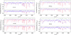 |
Fig. 2. Region from 5229 to 5285 Å of uncorrected disentangled spectra of the primary (top) and the secondary (bottom) components of AL Ari, AL Dor, FM Leo and BN Scl with selected spectral lines identified. The red lines denote the atmosphere models fits to the observed spectra (blue). The rotational broadening of the absorption lines is easily visible in AL Ari and BN Scl. |
Best-fitting final parameters of model atmospheres matching the observed spectra.
The Teff values of the components derived here are consistent to within 1σ with those derived from photometric colours (compare Tables 5 and 6). The only exception is the Teff of the primary component of AL Ari where this difference is larger than 2σ. Fortunately, for AL Ari we secured three spectra on 2014 December 14, during the total phase of the secondary eclipse when the pure spectrum of the primary component was visible. By co-adding them we obtained one spectrum with S/N ∼ 80. The use of the single mode of GSSP gives for this case Teff = 6396 ± 80 K, in 1σ agreement with the Teff derived from photometric colours. The remaining parameters ([M/H], ξ, ζ⋆, Vrot sin i) are consistent to within 1σ with parameters obtained with the GSSP_binary module.
Temperatures of components derived from intrinsic colours.
For the systems analysed in this work we obtain generally slightly subsolar metallicities, with the exception of AL Ari for which we find a significantly subsolar value ([M/H] ∼ −0.4 dex; see Table 5). In all cases we find that the stars rotate synchronously. In the case of AL Dor taking the rotational velocity and the macroturbulence simultaneously as free parameters leads to unrealistically low values for the former and high values for the latter. Therefore, during the fitting process, we fixed the values of Vrot sin i to the expected values for synchronous rotation (3.7 km s−1). Due to the faster rotation of the components of BN Scl, it was not possible to obtain reliable values of the macroturbulent velocity. GSSP returned unrealistically low best-fit values of ζ with large errors (Table 5). Therefore, we adopted ζ = 5 km s−1 based on data from the literature (Gray et al. 2001; Smalley 2014; Sheminova 2019).
4. Initial photometric analysis
4.1. Interstellar extinction
We used extinction maps (Schlegel et al. 1998) with the recalibration by Schlafly & Finkbeiner (2011) to determine the reddening in the direction of all four eclipsing binaries. We followed the procedure described in detail in Suchomska et al. (2015) assuming the distances from Gaia EDR3 (Gaia Collaboration 2021). Additionally, we used the three-dimensional interstellar extinction map STILISM (Capitanio et al. 2017). Finally, we adopted the average as the extinction estimate to a particular system.
4.2. Colour–temperature calibrations
To estimate the Teff values of the eclipsing components we collected multi-band magnitudes of the systems. We use 2MASS (Cutri 2003) as a good source for infrared photometry and the magnitudes were converted into appropriate photometric systems using transformation equations from Bessell & Brett (1988) and Carpenter (2001). The reddening (Sect. 4.1) and the mean Galactic interstellar extinction curve from Fitzpatrick & Massa (2007) assuming RV = 3.1 were combined with light ratios from the WD code in order to determine the intrinsic colours of the components. We determined the effective temperatures from a number of colour–temperature calibrations for a few colours: B − V (Alonso et al. 1996; Flower 1996; Ramírez & Meléndez 2005; González Hernández & Bonifacio 2009; Casagrande et al. 2010), V − J, V − H (Ramírez & Meléndez 2005; González Hernández & Bonifacio 2009; Casagrande et al. 2010), and V − K (Alonso et al. 1996; Houdashelt et al. 2000; Ramírez & Meléndez 2005; Masana et al. 2006; González Hernández & Bonifacio 2009; Casagrande et al. 2010; Worthey & Lee 2011). For calibrations having the metallicity terms we assumed the metallicity derived from the atmospheric analysis; see Table 5. The resulting temperatures were averaged for each component and are reported in Table 6. Usually our colour temperatures are about 1σ lower than the temperatures derived from atmospheric analysis in Sect. 3.3.2.
4.3. Adopted temperatures
Precise determination of the Teff values is very important in our approach because we did not adjust the limb-darkening coefficients during a fitting of light curves. Instead, these coefficients are automatically calculated for a given set of surface atmospheric parameters (Teff, log g) using tables from van Hamme (1993). Surface gravities are well determined internally within the WD code, but to set the Teff scale we need external information. The Teff scale was set by fixing the surface Teff of the primary star, T1, to the average of two previous Teff determinations (Sects. 3.3.2 and 4.2). The adopted T1 in all cases is well within the 1σ uncertainty of both Teff determinations. Subsequently, the Teff of the secondary, T2, was scaled according to T1 during the light-curve analysis with the WD code.
4.4. Analysis of minima times
For the purpose of the analysis we used a collection of minima times from the TIDAK database (Kreiner 2004). We augmented the data with minima times determined from the K2 and TESS light curves. Because of the continuous coverage and high photometric precision, the times of minimum derived from K2 and TESS light curves for AL Dor, FM Leo, and BN Scl are usually one or even two orders of magnitude more precise than those available in TIDAK.
4.4.1. AL Ari
The case of AL Ari was discussed by Kim et al. (2018) who fitted a model with apsidal motion and the light time effect (LITE) caused by an invisible companion to the minima times. They derived an apsidal period of U ≈ 6200 yr and found a very eccentric orbit for the third body with an orbital period of ∼90 yr. We repeated the analysis, but used increased uncertainties for some of the minima times reported. Because of the relatively short time-span of observations, instead of fitting a full third-body orbit (five more free parameters) we fitted a model with only a quadratic term (proportional to the first derivative of the sidereal period PS) and the apsidal motion. The computed minima times are:
where T0 is the reference epoch, E is an epoch number,  , the anomalistic period
  , j = 1 for primary and j = 2 for secondary eclipses, ω is the longitude of periastron and Ṗ = dPS/dt. The mean period
  was set to 3.747455 d and the orbital eccentricity was set to e = 0.051. For the coefficients A1, 2, 3 we used Eqs. (16)–(18) from Giménez & Bastero (1995), where we set cot2i = 0, because the orbital inclination of AL Ari is very close to 90°. Altogether we fitted five free parameters: T0, P, the linear period change term b, ω at T0, and the rate of advance of the periastron longitude
  .
.
The ephemeris is:

Figure 3 shows our solution. A significant apsidal motion can be noticed with  deg cycle−1 which is a value very close to that reported by Kim et al. (2018): 5.9 × 10⁻⁴ deg cycle−1. The first derivative of the orbital period is quite well constrained to be Ṗ = (6.34 ± 0.15) × 10−10 d cycle−1. Interpreting this change in terms of LITE, the expected radial-velocity acceleration of the barycentre of AL Ari induced by a third body is
  m s−1 cycle−1, which corresponds well with the value derived in Sect. 3.1 from the radial-velocity drift.
 |
Fig. 3. O − C diagrams of minima times. A linear term and, in case of AL Ari also a quadratic term, has been subtracted. Dark grey filled circles correspond to primary minima, and light grey ones to secondary minima. The inset in the panel for AL Dor shows the residuals of the model fit. |
4.4.2. AL Dor
This system shows a very slow apsidal motion. To fit the times of minimum we used a model with apsidal motion and a constant orbital period:

where the coefficients A are given by Eqs. (16)–(19) in Giménez & Bastero (1995). We set the eccentricity to e = 0.195 and fitted for four free parameters: T0, P, ω at T0, and  .
.
The solution is presented in Fig. 3. The inset shows residuals of our fit to the minima times determined from TESS photometry. Without the apsidal motion term these residuals show a small systematic trend. The resulting ephemeris is:

The rate of periastron advance is (1.330 ± 0.005)×10−4 deg cycle−1, corresponding to an apsidal motion period of U = 110 500 ± 400 yr.
4.4.3. FM Leo
As the orbit is practically circular we fitted a simple linear ephemeris to both types of minimum:
The residuals do not show any noticeable trends (see Fig. 3). The ephemeris for FM Leo is:

4.4.4. BN Scl
The orbit of the system is slightly eccentric and we fitted a linear ephemeris with no apsidal motion or LITE terms:

where the coefficient A is given by Eq. (16) in Giménez & Bastero (1995). The eccentricity and longitude of periastron were set to values from the full analysis of the light and velocity curves (Sect. 5.3.4). The resulting ephemeris is:

5. Analysis of combined light and radial-velocity curves
For analysis of the eclipsing binaries we make use of the Wilson-Devinney program version 2007 (Wilson 1979, 1990; van Hamme & Wilson 2007)2, equipped with a Python wrapper.
5.1. Initial parameters
We fixed the Teff of the primary component during analysis to the average of the Teff values derived from the colour–temperature calibrations and the atmospheric analysis. In all cases those two determinations are consistent to within 1σ. The standard albedo and gravity brightening coefficients for convective stellar atmospheres were chosen. The stellar atmosphere option was used (IFAT1=IFAT2=1), radial-velocity tidal corrections were automatically applied (ICOR1=ICOR2=1), and no flux-level-dependent weighting was used. We assumed synchronous rotation for both components in all systems. The epoch of the primary minimum was set according to results of the O − C diagram analysis. Both the logarithmic (Klinglesmith & Sobieski 1970) and square root (Diaz-Cordoves & Gimenez 1992) limb-darkening laws were used, with coefficients tabulated by van Hamme (1993).
5.2. Fitting model parameters
With the WD binary star model we fitted the available light curves and a radial-velocity curve for each component simultaneously. We assumed a detached configuration in all models and a simple reflection treatment (MREF = 1, NREF = 1). Each observable curve was weighted only by its rms through comparison with the calculated model curve. We adjusted the following parameters during analysis: the orbital period Porb, the semimajor axis a, the mass ratio q, both systemic radial velocities γ1, 2, the phase shift ϕ, the eccentricity e, the argument of periastron ω, the orbital inclination i, the temperature of the secondary T2, the modified Roche potentials Ω1, 2 —corresponding to the fractional radii r1, 2— and the luminosity parameter L1. Additionally, we fitted for third light l3. The best models were chosen according to their reduced χ2 and a lack of significant systematic trends in the residuals.
The statistical (formal) errors on model parameters were estimated with the Differential Correction subroutine of the WD code. To the formal errors, we added a mean correction on every model parameter from the last three iterations, provided that the iterated models were close to the final solution (to within 1σ). We also compared numerical values of model parameters obtained with different limb-darkening laws and with a third light accounted for. Averaged differences were added in quadrature to the total error budget.
5.3. Analysis details and results
5.3.1. AL Ari
We used three Strömgren bands (v, b and y) because the light curve in the u filter is significantly more noisy and also has additional systematic offsets in the secondary minimum due to unfavourable sky conditions. The grid fineness parameters were set to N1=N2=50. In the beginning we solved the radial velocities and light curves separately to obtain the best individual solutions. We then combined the light curves with the velocimetry to obtain a simultaneous solution with the WD code. As AL Ari has a notable apsidal motion and acceleration of its barycentre due to an invisible companion, we included two additional free parameters in the fit: the first derivative of the orbital period DPDT= Ṗ (dimensionless) and the first derivative of the longitude of periastron DPERDT (rad day−1). We set the initial epoch at the mid-time around which the Strömgren light curves were obtained: May 1998. Because there were many correlations between parameters in the beginning we set DPERDT = 2.7 × 10⁻⁵ based on results from the analysis of minima times. After several iterations we included this as a free parameter.
The final solution is consistent with results from the minima times analysis, however the resulting orbital period change is five times faster. It is probable that more complicated period changes (caused by a tertiary) beyond the simple linear model we used are responsible for this. We also tested for the presence of third light. However, its inclusion did not improve the solution and the fitted values of l3 were consistent with zero in all bands. We could only put an upper limit of l3 < 1% for the light curves. The parameters of the final solution are given in Table 7. The best model fit to the y-band light curve is presented in Fig. 4, while the best model fit to the radial velocities is shown in Fig. 5. The radial-velocity rms of the primary component is consistent with expected precision of HARPS in EGGS mode, but the secondary shows significantly larger rms than expected.
 |
Fig. 4. WD model fits to the photometric observations. |
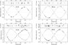 |
Fig. 5. WD model fits to the radial-velocity curves. |
Results of the final analysis with the WD code.
The configuration of the system is well detached. The tidal deformations, defined as (rpoint − rpole)/rmean, are just 0.3% and 0.1% for the primary and the secondary, respectively. The absolute dimensions of the system were calculated using nominal astrophysical constants advocated by IAU 2015 Resolution B3 (Prša et al. 2016) and are presented in Table 8. Unlike the other systems analysed in this work, the components of AL Ari have quite different masses, sizes, temperatures, and luminosities.
Physical parameters of the stars.
We estimated the spectral type of the system to be F6 V + G7 V using tables by Pecaut & Mamajek (2013). This is consistent with the spectral type of F8 estimated from photographic observations (Hill & Schilt 1952).
5.3.2. AL Dor
We combined the TESS light curve with our velocimetry from HARPS and CORALIE spectra. We used the grid fineness parameters N1=N2=60, the highest available value in the 2007 version of the WD code. To represent the TESS band we used the Cousins I-band (filter 16 in the WD code). Our analysis of the TESS photometry of the AI Phe system (Maxted et al. 2020) showed that approximating the TESS band with the IC band leads to systematic errors in the fractional radii which are smaller than 0.05% and can therefore be neglected.
The logarithmic law of the limb darkening was applied to both stars. Because of the apsidal motion there is a small orbital phase shift between the velocimetry and photometry. To achieve the best solution we first solved only the velocimetry to derive the orbital parameters, and then used them as input to derive a photometric model using only the photometry. We iterated this step several times until all parameters of the two models were the same, with the exception of ϕ and ω. We then ran several simultaneous iterations setting DPERDT free. The resulting value of 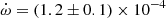 deg cycle−1 is in full agreement with the result from the minima times analysis. A summary of the model parameters is given in Table 7. Adjusting l3 does not improve the solution, as the WD code returns small negative values of l3 without a decrease of residuals. We assumed l3 = 0.
The components of AL Dor are extremely similar to each other (Table 8): their masses and temperatures are the same to within 0.1% and the radii to within 0.6%. Because of this the system is valuable for very precise calibration of the surface brightness–colour relations: the components have the same colours and the flux ratio does not change significantly for a wide range of wavelengths.
We estimated the spectral type of the system as F9 V + F9 V based on the calibration by Pecaut & Mamajek (2013), which is consistent with the spectral type of F8 V given by Houk & Cowley (1975). Our mass measurements coincide well with the measurements from Gallenne et al. (2019) because we used the same velocimetry, but the errors on our masses are larger by a factor of 1.5. We note that we use a different definition of the primary star, because the eclipse of the less massive and smaller star is slightly deeper than the other eclipse.
5.3.3. FM Leo
We fitted the light and radial-velocity curves simultaneously using the grid fineness parameters N1=N2=60. To represent the Kepler band within the WD code, we used the Cousins R band (filter 15 in the WD code) which has very similar effective wavelength. For our initial solution we used parameters from Ratajczak et al. (2010). We quickly found that a circular orbit produces small systematic trends in the residuals during both eclipses, and so we set the eccentricity and the longitude of periastron as free parameters during the fitting. Initially, we set the third light to zero and looked for the best solution with the logarithmic law of the limb darkening (parameter LD = −2 for both components). In order to properly recreate the out-of-eclipse light changes, which have an amplitude of 0.6 mmag, we also fitted the albedo parameters of both stars, A1 and A2. The best light curve solution had a very small rms of 0.283 mmag, but there were still small systematic errors noticable in the eclipses at a level of ∼300 ppm. We also tried the square root law of the limb darkening (LD = −3) and obtained a slightly better solution with an rms of 0.275 mmag but the systematic residuals persisted, albeit somewhat smaller (∼200 ppm). Finally, we let third light be a free parameter of the fit. Surprisingly, a small third light l3 = 0.005 was detected with a high significance of 12σ. The best solution with l3 has no systematic residuals within the primary minimum and within the secondary minimum they are of order of only ∼100 ppm (see the upper right panel of Fig. 4). The model parameters are given in Table 7. We note also an anomalous albedo for both components of FM Leo, which is expected to be 0.5 in case of a convective atmosphere, but it is significantly lower. The reason for that is unclear.
It is interesting that the best orbital solution we found still has a very small eccentricity. It is not an artefact or a spurious detection, because only a non-circular orbit removes the systematic residuals in eclipses. Assuming that FM Leo is a triple system (see discussion below), the tidal forces of the tertiary would induce perturbations to the inner orbit of FM Leo, producing tiny but noticeable deviations from circularity.
The components, as in the case of AL Dor, have very similar temperatures, but they differ slightly in mass and radius (see Table 8). Maxted & Hutcheon (2018) already pointed out that this system can be very valuable for testing stellar models, because both components are slightly evolved and have masses in a range where the core-overshooting starts to play an important role (e.g., Claret & Torres 2019). Our photometric parameters are consistent to within 2σ with the parameters found by Maxted & Hutcheon (2018) who solved the long-cadence K2 data. A comparison with physical parameters reported by Ratajczak et al. (2010) shows remarkably good agreement, although our parameters are an order of magnitude more precise. The masses reported by Sybilski et al. (2018) are consistent with our values to within 2σ, while the radii reported by these latter authors are very different. The likely reason of this discrepancy is the use of the preliminary light curve of FM Leo from the Solaris project by Sybilski et al. (2018) (K. Hełminiak, priv. comm.). We estimate the spectral type of the system to be F6 V + F6 V, which compares well with the estimate of F7 V from Houk & Swift (1999).
The third light. We investigated possible sources of the positive third light in the Kepler light curve. It would correspond to a star with a brightness of R ∼ 13.9 mag. Within a radius of 12″ around FM Leo there is no source of light brighter than R ∼ 20 mag in the Gaia DR2 catalogue or in any other deep catalogue of stellar sources. If this third light comes from a physically bound companion, it would have an absolute magnitude of MR = 8.0 mag, corresponding to a K9 V star. We looked for a sign of the third light in our highest-S/N HARPS spectra taken around quadrature using the broadening function. We used a template corresponding to a K9 V star. In the red part of the spectrum there is no trace of absorption lines from a possible companion to within a limit of ∼0.5% of the total light of the system.
FM Leo was reported to have a quite significant proper motion anomaly (Kervella et al. 2019) and was flagged as a ‘binary’. In our case it would mean ‘a triple’ with a relatively short tertiary orbital period. However, orbital phases calculated separately from radial-velocity curves and the light curve are in perfect agreement. Also, our analysis of the O − C diagram (Sect. 4.4) does not show any trace of a change of the orbital period. We can also consider one other possibility: that a use of approximate limb-darkening laws representing changes of the surface brightness over a stellar disc leads to the residuals. As noted above, a shift from the logarithmic law to the square root law helped to reduce the systematic residuals in eclipses. The version 2007 of the WD code unfortunately does not provide fitting of the limb-darkening coefficients of two-parametric laws, and so for the time being we leave the question of the source of the residuals open. For the purpose of the current work we assume that the third light is real and comes from a K9 V companion star on a wide orbit.
The Doppler beaming. The upper panel of Fig. 6 shows a close-up of the out-of-eclipse flux changes of FM Leo. Although the best model represents the flux changes very well, we note that during the first quadrature FM Leo is on average brighter by ∼0.1 mmag than during the second quadrature. As the WD model includes flux changes due to tidal deformation of the components and the mutual reflection, persistent systematic residuals of about 120 ppm come most probably from Doppler boosting. To calculate the expected Doppler boosting signal we used Eq. (9) from Placek (2019). We estimated the beaming factor for Teff = 6300 K and log g = 4.0 to be B = 3.6 ± 0.2 from Fig. 2 in Placek (2019). The flux changes due to the Doppler boosting are plotted in the bottom panel of Fig. 6 together with the binned residuals. The agreement is remarkable, suggesting that the detection is real and significant at the 3σ level. To our knowledge this is the first detection of the Doppler beaming in a binary system consisting of two similar main sequence stars.
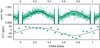 |
Fig. 6. Top: out-of-eclipse flux changes of FM Leo, with the best-fit model from WD overplotted. The ellipsoidal modulation and the reflection is included in the model. Bottom: residuals binned to steps of 0.05 in phase. The theoretical light variation due to Doppler beaming is overplotted. |
Short-cadence versus long-cadence data. Having both sets of data for FM Leo we made a high-precision test of solving both sets of photometry independently and comparing the results. We solved the full long-cadence data for FM Leo in a similar manner to the short cadence data. In order to account for the phase smearing which flattens out the brightness variations we used an iterative approach to correct the long-cadence light curve (LCLC). In case of FM Leo, one photometric point of LCLC corresponds to the integration time of ∼0.003 orbital phases; that is a significant part of the eclipse duration: almost 7%. Based on the preliminary WD model obtained from LCLC, we determined corrections as follows. We generated a synthetic normalised light curve with very dense coverage of the orbital phase (5000 points). Based on this for every synthetic point we calculated a mean synthetic flux corresponding to the phase smearing of 0.003. The difference of the two is a correction which we applied to every point of the phased LCLC. We then solved the corrected light curve to derive an improved model. We iterated this scheme three times until the resulting differences between the new and old corrections were below 200 ppm.
Both model solutions, one obtained by directly fitting the short-cadence light curve (SCLC) and one obtained by fitting the corrected LCLC are in perfect agreement: not only are the synthetic light curves essentially the same but also the resulting photometric model parameters are the same to within the uncertainties. As already pointed out by Maxted & Hutcheon (2018), we note that the residuals of the LCLC solution during eclipse are twice as high as the out-of-eclipse residuals. However, the SCLC light curve shows the same magnitude of residuals within and outside eclipse. We conclude that this iterative scheme can be reliably applied to solve K2 and TESS light curves of eclipsing binaries for which only long cadence data are available.
5.3.4. BN Scl
Because of the small spots affecting the light curve of BN Scl, we used only a part of the TESS photometry when the spot activity was the smallest. We did not fit spots on any of the components, but instead allowed to fit both albedo parameters A1 and A2. We used the grid fineness parameters N1=N2=60 and the logarithmic limb-darkening law. The photometry and velocimetry were solved simultaneously. The albedo of the primary is very low and consistent with zero (see Table 7), most probably because of the presence of the spots. The best-fit model presented in Fig. 4 still shows the small systematic residuals of ∼500 ppm near mid-eclipse during the secondary minimum. A use of the square root law for the limb darkening does not provide any improvement to the solution. There is a faint, red star ∼8 arcsec to the southwest of BN Scl which is on the edge of the TESS photometric aperture: TIC 155543721, with an estimated TESS magnitude of 15.8 (0.1% of the flux of BN Scl). Allowing the third light to be a free parameter of the light curve fit does not help to reduce the residuals and the returned values of l3 are consistent with zero. We put the upper limit for the l3 as 0.1% in the TESS light curve. Most probably the presence of small spot(s) affects the model fit and produces small systematic residuals at the secondary minimum (see Fig. 7).
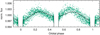 |
Fig. 7. Out-of-eclipse flux changes of BN Scl, with the best-fit model from WD overplotted. The deviations from the best fit at the orbital phases from 0.4 to 0.8 due to the spot activity can reach ∼1.5 mmag. |
The components are slightly evolved, especially the primary. The tidal distortion amounts to 0.6% for the primary and 0.3% for the secondary. The system may be very valuable for testing models of stellar evolution as the components differ significantly in their masses and are below the 2 M⊙ limit where core overshooting may depend strongly on mass. The metallicity of the system is significantly subsolar. The spectral types of components are F7 V + F8 V, in perfect agreement with the estimate of F7 V from Houk (1982).
6. Calibration of new surface brightness–colour relations.
In our previous work (Graczyk et al. 2017) we investigated the surface brightness–colour relations derived solely from eclipsing binary stars using a mixture of HIPPARCOS (van Leeuwen 2007) and Gaia DR1 parallaxes (Gaia Collaboration 2016). Here we derive new relations utilising much more precise Gaia EDR3 parallaxes (Gaia Collaboration 2021).
6.1. Sample
We used a compilation of eclipsing binary stars from Graczyk et al. (2019), with updated parameters on three systems: AL Dor, AL Ari, and FM Leo (this paper). We added four new systems to the sample: BN Scl, β Aur, NN Del, and V1022 Cas. In the case of β Aur, we used parameters from Southworth et al. (2007) and Behr et al. (2011) while for NN Del we adopted masses from Gallenne et al. (2019) and photometric parameters from Sybilski et al. (2018). For AI Phe we adopted very precise parameters from recent papers by Gallenne et al. (2019) and Maxted et al. (2020). Parameters for V1022 Cas were adopted from a number of recent works (Fekel et al. 2010; Lester et al. 2019; Southworth 2020). In order to minimise the interstellar extinction and the Gaia zero-point uncertainties we set a distance limit of 200 pc corresponding to the trigonometric parallaxes ϖ > 5 mas. We also put a precision limit of 1.5% on the relative radii of both components, resulting in a sample of 27 systems. For each we downloaded the Gaia EDR3 parallaxes and auxiliary parameters from the Gaia Archive3. None of the selected systems have a RUWE parameter4 larger than 1.4, which would signify a problematic astrometric solution. For β Aur we used the HIPPARCOS parallax (van Leeuwen 2007). In the final sample of 28 systems the median errors on the parallaxes and absolute radii are 0.3% and 0.6%, respectively.
6.2. Geometric distances
Gaia EDR3 significantly improves on Gaia DR2 in terms of the precision and the accuracy of the astrometry (Lindegren et al. 2021b). In particular, the zero-point shift of Gaia EDR3 parallaxes (the parallax bias) was determined (Lindegren et al. 2021a) as a function of the G magnitude (photgmeanmag in the Gaia Archive), a colour and an ecliptic latitude β (ecllat). As a colour parameter, rather than using the colour index GBP − GRP, an effective wavenumber νeff (nueffusedinastrometry) was used in the five-parameter astrometric solutions and an astrometric pseudo-colour  (pseudocolour) in the six-parameter astrometric solutions. In Gaia EDR3, quasars have a median parallax of −17 μas and in general brighter and bluer objects have a larger negative parallax bias. The bias function Z(G, νeff, β) is provided separately for the five- (Z5) and six-parameter (Z6) solutions as a Python module zero-point, which is available via the Gaia web pages5.
In order to calculate the new surface-brightness–colour relations we used parallaxes corrected for the parallax bias. The average change of parallax in our sample due to this correction is just −0.3% thanks to the proximity of the systems (ϖ > 5 mas).
6.3. Photometry
We used our compilation (Graczyk et al. 2019) as a source of optical Johnson B and V magnitudes. For new systems we used mean magnitudes from a number of catalogues available in the VizieR catalogues access tool. GBP and G EDR3 photometry was downloaded from the Gaia Archive. For near-infrared photometry, we used 2MASS magnitudes from Cutri (2003) which were corrected for the presence of eclipses. The corrections were calculated from synthetic light curves in JHK bands using our WD models of the systems. In case of β Aur we used Johnson photometry from a compilation by Ducati (2002) transformed into the 2MASS photometric system.
6.4. The third light
Intrinsic colours of the components were calculated in each band from the light ratios we determined using the WD code. However, in a few cases we had to account for the third light. Two systems are confirmed triples: AI Phe and AL Ari. A characteristics of the third light in the TESS light curve of AI Phe was presented by Maxted et al. (2020), with a suggestion that a companion is a late-K dwarf. For this paper, we assumed that the companion is a K9 V star and we subsequently computed its contribution to the various bands using an online table of intrinsic colours of main sequence stars6 (Pecaut & Mamajek 2013). The expected contribution of the companion to the total flux in the K band is 1.6%, and in the optical is less than 0.2% (B band).
In the case of AL Ari we can only put an upper limit on the third light of 1% in the V band. At the distance of AL Ari (∼140 pc) this means that the spectral type of the companion would be later than K8 V. However, the proper-motion anomaly (Kervella et al. 2019) and the small acceleration of the system’s barycentre suggest a lower-mass companion. For the purpose of this work we do not assume any parameters for the companion and we set l3 = 0 in all bands.
Another system, FM Leo, is a suspected triple because of the third light, which we detected in the K2 light curve and by its significant proper-motion anomaly. We calculated the contribution of the putative companion star (a K9 dwarf) in different bands in a similar manner to AI Phe. In the K band the expected contribution amounts to 3.3% of the total flux of the system, while in the B band only to 0.15%. For both AI Phe and FM Leo we used these contributions to correct the intrinsic colours and the surface-brightness parameters of their components.
6.5. Results
Our sample of eclipsing binaries covers stars with spectral types from B7 V (the primary of GG Lup) down to M1 V (the secondary of V530 Ori). However, these extremes are much bluer and much redder than the rest of the sample and all calibrations were done in smaller colour ranges corresponding to spectral types ranging from B9 V (the secondary of GG Lup) down to K0 IV (the secondary of AI Phe). All components are main sequence stars with the exception of a small number of subgiants. In the sample, the mean surface gravity is log g = 4.22 and the lowest value is log g = 3.6.
The surface brightness parameter S was calculated for each band using Eq. (5) from Hindsley & Bell (1989):
where m0 is the intrinsic magnitude of a star in given band and θLD is the limb-darkened angular diameter expressed in milliarcseconds. The angular diameters were calculated using:

where R is the stellar radius expressed in nominal solar radii ℛ⊙ (Prša et al. 2016).
The colours of the components were calculated from the dereddened observed magnitudes and the light ratios in different bands provided by the WD models. Because for a spectral type ∼A0 the SBCRs show significant non-linearity (see e.g., Challouf et al. 2014), we decided to fit fifth-order polynomials. Fits were done using the orthogonal distance regression. Figure 8 shows calibrations of the surface brightness parameter S in four filters (B, V, GBP and G) against the optical-infrared colours. All SBCRs calibrated against the 2MASS K band show the smallest residuals with rms of ∼0.025 mag (∼1%). Notably the SBCRs calibrated with the 2MASS J and H bands show considerably larger residuals by a factor of approximately two. The likely reason for this is the precision of the 2MASS photometry itself, which reaches 1% in the K band and only 2% in the J and H bands. Currently, the quality of the infrared photometry is the main limiting factor to the precision with which we can calibrate the SBCRs. Another significant source of residuals are the radii of eclipsing binary components, which are known with a precision of 1–2% for a number of systems.
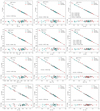 |
Fig. 8. SBCRs derived for eclipsing binary stars and calibrated for Johnson B, V filters, and Gaia EDR3 GBP and G filters. Infrared magnitudes are expressed in the 2MASS system. |
Table 9 presents coefficients of the fifth-order polynomial fits over the colour range in which a particular SBCR can be safely used. Instead of giving uncertainties of fitted coefficients we give information about the precision of the predicted stellar angular diameter.
Coefficients of polynomial fits to the surface-brightness parameter S in Johnson B and V and Gaia GBP and G bands for dwarfs and subgiants.
Gaia EDR3 does not account for binary solutions and so systems with larger photocentre movement (PHM) may have their parallaxes affected, and this will contribute to the scatter in the SBCRs. In our sample ten systems have significant amplitudes of the PHM, that is, they are much larger than the errors of parallaxes. Gallenne et al. (2019) determined precise orbital parallaxes for four systems in our sample using interferometry, and these are consistent to within 1σ with Gaia parallaxes for AL Dor and AI Phe (which have an insignificant PHM) but disagree at the 2.5σ level for KW Hya and NN Del (which have a significant PHM). On the other hand, only NN Del has a large PHM amplitude (8% of the Gaia parallax), whilst for the rest of the sample the amplitude is smaller than 3% with a median of just 0.6%.
6.6. Comparison with previous calibrations
We compared the SBCR from Table 9 for SV and (V − K) against a number of published calibrations from the literature. As most relations are usually calibrated using the Johnson K band we transformed the 2MASS photometry into the Johnson photometric system. In Fig. 9 we plot our fit and a few calibrations based on interferometric measurements of stellar angular diameters (Kervella et al. 2004; Challouf et al. 2014; Boyajian et al. 2014; Salsi et al. 2020). The calibrations based on the interferometry have precision of about 2–3% for dwarfs in the colour range of our sample. The SBCR derived from eclipsing binary stars and interferometry show very good consistency, with mean offsets below 2%. Especially, the relation by Kervella et al. (2004) is very consistent with our polynomial fit: in a whole range of (V − K) colour the differences between the two relations are smaller than 1.5%. The exception is the relation by Challouf et al. (2014) in a colour range of 0.1–1.0 where there is a systematic offset of about 3%. The reason of the discrepancy is not clear to us at the moment, but selection effects are a possible explanation.
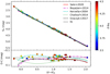 |
Fig. 9. Comparison of different V-band surface brightness calibrations onto Johnson (V − K) colour. |
We compared also our new SBCR with the linear relation derived for the (V − K) colour by Graczyk et al. (2017). The rms of our new relation is almost three times smaller than the previous one. The previous calibration shows a systematic difference of about 1.5%, which is well within the precision of the calibration (2.7%). The reason for the offset is that in the previous calibration we used less precise and accurate parallaxes from HIPPARCOS and Gaia DR1.
7. Final remarks
We present the results of a detailed analysis of four well-detached eclipsing binary systems. We reach very high precision in the determination of the fundamental physical parameters of the component stars. This was possible thanks to the high quality of ground- and space-based photometry and spectroscopy we used, and a careful multi-step analysis incorporating multiple consistency checks for the derived parameters.
Some of the analysed systems, for example AL Ari, may become benchmark stars due the high precision of the derived parameters and the number of different techniques used in their investigation. AL Dor is a model system for calibration of the SBCR because its components are almost identical. FM Leo and BN Scl can be very useful for testing the strength of convective core overshooting in stars for a mass range between 1 and 2 M⊙.
The main result of this paper is a new and very precise calibration of the SBCRs using Gaia EDR3 parallaxes. We have achieved this precision for the first time by using only eclipsing binary stars with secure geometric distances. Although in our previous paper (Graczyk et al. 2017) we used a similar methodology, the relatively low precision of the available parallaxes forced us to use photometric distance priors which led to small systematic biases in the derived angular diameters.
We expect the new SBCRs to be a useful tool for predicting the angular diameters of stars, especially as we calibrated them using all-sky homogenous photometric systems: 2MASS and Gaia. One of the immediate applications is the determination of the absolute zero-point shift of the Gaia EDR3 parallaxes in a way similar to the one presented by Graczyk et al. (2019) for Gaia DR2.
There remains room for improvement of the calibrations. First, the colour range over which the calibrations are applicable could be extended by including in the sample more nearby eclipsing binary systems with early-type components (late B and A type stars) or late-G type components. Second, the uncertainties in the infrared photometry could be driven down via multi-epoch observations with a relative precision of about 1% in the J and K bands. Third, the sample size could be increased via a re-analysis of a subsample of known systems for which new high-quality light curves from K2 or TESS are available. Lastly, a possible parallax bias could be removed by utilising future Gaia data releases in which binary motion will be included in astrometric solutions. By implementing all these steps we could expect to reach subpercentage precision in the predicted angular diameters of stars for the first time.
Acknowledgments
This work has made use of data from the European Space Agency (ESA) mission Gaia (https://www.cosmos.esa.int/gaia), processed by the Gaia Data Processing and Analysis Consortium (DPAC, https://www.cosmos.esa.int/web/gaia/dpac/consortium). Funding for the DPAC has been provided by national institutions, in particular the institutions participating in the Gaia Multilateral Agreement. We are grateful to J. V. Clausen, B. E. Helt, and E. H. Olsen for making their unpublished uvby photometric data available to us. The research leading to these results has received funding from the European Research Council (ERC) under the European Union’s Horizon 2020 research and innovation program (grant agreement No. 695099) and from the National Science Center, Poland grants MAESTRO UMO-2017/26/A/ST9/00446 and BEETHOVEN UMO-2018/31/G/ST9/03050. We acknowledge support from the IdP II 2015 0002 64 and DIR/WK/2018/09 grants of the Polish Ministry of Science and Higher Education. W. G. also gratefully acknowledges financial support for this work from the BASAL Centro de Astrofisica y Tecnologias Afines BASAL-CATA (AFB-170002), and from the Millenium Institute of Astrophysics (MAS) of the Iniciativa Cientifica Milenio del Ministerio de Economia, Fomento y Turismo de Chile, project IC120009. P. K. and N. N. acknowledge the support of the French Agence Nationale de la Recherche (ANR), under grant ANR-15-CE31-0012-01 (project UnlockCepheids). MT acknowledges financial support from the Polish National Science Center grant PRELUDIUM 2016/21/N/ST9/03310. The research leading to these results has (partially) received funding from the KU Leuven Research Council (grant C16/18/005: PARADISE), from the Research Foundation Flanders (FWO) under grant agreement G0H5416N (ERC Runner Up Project), as well as from the BELgian federal Science Policy Office (BELSPO) through PRODEX grant PLATO. This research has made use of the VizieR catalogue access tool, CDS, Strasbourg, France (DOI : 10.26093/cds/vizier). The original description of the VizieR service was published in 2000, A&AS 143, 23. We used the uncertainties python package.
References
- Alonso, A., Arribas, S., & Martínez-Roger, C. 1996, A&A, 313, 873 [Google Scholar]
- Barnes, T. G., Evans, D. S., & Parsons, S. B. 1976, MNRAS, 174, 503 [NASA ADS] [CrossRef] [Google Scholar]
- Behr, B. B., Cenko, A. T., Hajian, A. R., et al. 2011, AJ, 142, 6 [NASA ADS] [CrossRef] [Google Scholar]
- Bessell, M. S., & Brett, J. M. 1988, PASP, 100, 1134 [NASA ADS] [CrossRef] [Google Scholar]
- Boyajian, T. S., van Belle, G., & von Braun, K. 2014, AJ, 147, 47 [NASA ADS] [CrossRef] [Google Scholar]
- Capitanio, L., Lallement, R., Vergely, J. L., et al. 2017, A&A, 606, A65 [NASA ADS] [CrossRef] [EDP Sciences] [Google Scholar]
- Carpenter, J. M. 2001, AJ, 121, 2851 [NASA ADS] [CrossRef] [Google Scholar]
- Casagrande, L., Ramírez, I., Meléndez, J., Bessell, M., & Asplund, M. 2010, A&A, 512, A54 [NASA ADS] [CrossRef] [EDP Sciences] [Google Scholar]
- Challouf, M., Nardetto, N., Mourard, D., et al. 2014, A&A, 570, A104 [NASA ADS] [CrossRef] [EDP Sciences] [Google Scholar]
- Clausen, J. V., Helt, B. E., & Olsen, E. H. 2001, A&A, 374, 980 [NASA ADS] [CrossRef] [EDP Sciences] [Google Scholar]
- Claret, A., & Torres, G. 2019, ApJ, 876, 134 [Google Scholar]
- Coelho, P., Barbuy, B., Meléndez, J., Schiavon, R. P., & Castilho, B. V. 2005, A&A, 443, 735 [NASA ADS] [CrossRef] [EDP Sciences] [Google Scholar]
- Cutri, R. M., et al. 2003, VizieR, Online Data Catalogue, 2246 [Google Scholar]
- Diaz-Cordoves, J., & Gimenez, A. 1992, A&A, 259, 227 [Google Scholar]
- Ducati, J. R. 2002, VizieR Online Data Catalog: II/237 [Google Scholar]
- Fekel, F. C., Tomkin, J., & Williamson, M. H. 2010, AJ, 139, 1579 [Google Scholar]
- Fitzpatrick, E. L., & Massa, D. 2007, ApJ, 663, 320 [NASA ADS] [CrossRef] [EDP Sciences] [Google Scholar]
- Flower, P. J. 1996, ApJ, 469, 355 [Google Scholar]
- Gaia Collaboration (Prusti, T., et al.) 2016, A&A, 595, A1 [NASA ADS] [CrossRef] [EDP Sciences] [Google Scholar]
- Gaia Collaboration (Brown, A. G. A., et al.) 2021, A&A, 649, A1 [NASA ADS] [CrossRef] [EDP Sciences] [Google Scholar]
- Gallenne, A., Pietrzyński, G., Graczyk, D., et al. 2016, A&A, 586, A35 [NASA ADS] [CrossRef] [EDP Sciences] [Google Scholar]
- Gallenne, A., Pietrzyński, G., Graczyk, D., et al. 2019, A&A, 632, A31 [EDP Sciences] [Google Scholar]
- Giménez, A., & Bastero, M. 1995, Ap&SS, 226, 99 [NASA ADS] [CrossRef] [Google Scholar]
- González, J. F., & Levato, H. 2006, A&A, 448, 283 [NASA ADS] [CrossRef] [EDP Sciences] [Google Scholar]
- González Hernández, J. I., & Bonifacio, P. 2009, A&A, 497, 497 [NASA ADS] [CrossRef] [EDP Sciences] [Google Scholar]
- Graczyk, D., Maxted, P. F. L., Pietrzyński, G., et al. 2015, A&A, 581, A106 [NASA ADS] [CrossRef] [EDP Sciences] [Google Scholar]
- Graczyk, D., Smolec, R., Pavlovski, K., et al. 2016, A&A, 594, A92 [NASA ADS] [CrossRef] [EDP Sciences] [Google Scholar]
- Graczyk, D., Konorski, P., Pietrzyński, G., et al. 2017, ApJ, 837, 7 [Google Scholar]
- Graczyk, D., Pietrzyński, G., Gieren, W., et al. 2019, ApJ, 872, 85 [NASA ADS] [CrossRef] [Google Scholar]
- Graczyk, D., Pietrzyński, G., Thompson, I. B., et al. 2020, ApJ, 904, 13 [Google Scholar]
- Gray, D. F. 2005, The Observation and analysis of Stellar Photospheres (New York: Cambridge University Press) [Google Scholar]
- Gray, D. F., Graham, P. W., & Hoyt, S. R. 2001, AJ, 121, 2159 [NASA ADS] [CrossRef] [Google Scholar]
- Hill, S. J., & Schilt, J. 1952, Contributions from the Rutherford Observatory of Columbia University New York, 32, 1 [NASA ADS] [Google Scholar]
- Hindsley, R. B., & Bell, R. A. 1989, ApJ, 341, 1004 [NASA ADS] [CrossRef] [Google Scholar]
- Houdashelt, M. L., Bell, R. A., & Sweigert, A. V. 2000, AJ, 119, 1448 [Google Scholar]
- Houk, N. 1982, Michigan Catalogue of Two-dimensional Spectral Types for the HD stars. Volume_3. Declinations -40_0 to -26_0 (Houk, N. Ann Arbor, MI(USA): Department of Astronomy, University of Michigan), 12 + 390 [Google Scholar]
- Houk, N., & Cowley, A. P. 1975, in University of Michigan Catalogue of two-dimensional spectral types for the HD stars. Volume I. Declinations -90_ to -53_0, eds. N. Houk, & A. P. Cowley (Ann Arbor, MI (USA): Department of Astronomy, University of Michigan), 19 + 452 [Google Scholar]
- Houk, N., & Swift, C. 1999, in Michigan catalogue of two-dimensional spectral types for the HD Stars, eds. N. Houk, & C. Swift (Ann Arbor, Michigan: Department of Astronomy, University of Michigan), 5, 1999 [Google Scholar]
- Howell, S. B., Sobeck, C., Haas, M., et al. 2014, PASP, 126, 398 [NASA ADS] [CrossRef] [Google Scholar]
- Kazarovets, E. V., Samus, N. N., Durlevich, O. V., et al. 1999, Inf. Bull. Var. Stars, 4659, 1 [Google Scholar]
- Kervella, P., Thévenin, F., Di Folco, E., & Ségransan, D. 2004, A&A, 426, 297 [NASA ADS] [CrossRef] [EDP Sciences] [Google Scholar]
- Kervella, P., Arenou, F., Mignard, F., et al. 2019, A&A, 623, A72 [NASA ADS] [CrossRef] [EDP Sciences] [Google Scholar]
- Kim, C.-H., Kreiner, J. M., Zakrzewski, B., et al. 2018, ApJS, 235, 41 [NASA ADS] [CrossRef] [Google Scholar]
- Klinglesmith, D. A., & Sobieski, S. 1970, AJ, 75, 175 [Google Scholar]
- Koch, D. G., Borucki, W. J., Basri, G., et al. 2010, ApJ, 713, L79 [NASA ADS] [CrossRef] [Google Scholar]
- Kreiner, J. M. 2004, Acta Astron., 54, 207 [NASA ADS] [Google Scholar]
- Kruszewski, A., & Semeniuk, I. 1999, Acta Astron., 49, 561 [NASA ADS] [Google Scholar]
- Lacy, C. H. 1977a, ApJS, 34, 479 [NASA ADS] [CrossRef] [Google Scholar]
- Lacy, C. H. 1977b, ApJ, 213, 458 [NASA ADS] [CrossRef] [Google Scholar]
- Lester, K. V., Gies, D. R., Schaefer, G. H., et al. 2019, AJ, 157, 140 [Google Scholar]
- Lindegren, L., Klioner, S., Hernández, J., et al. 2021a, A&A, 649, A2 [EDP Sciences] [Google Scholar]
- Lindegren, L., Bastian, U., Biermann, B., et al. 2021b, A&A, 649, A4 [EDP Sciences] [Google Scholar]
- Masana, E., Jordi, C., & Ribas, I. 2006, A&A, 450, 735 [NASA ADS] [CrossRef] [EDP Sciences] [Google Scholar]
- Maxted, P. F. L., & Hutcheon, R. J. 2018, A&A, 616, A38 [NASA ADS] [CrossRef] [EDP Sciences] [Google Scholar]
- Maxted, P. F. L., Gaulme, P., Graczyk, D., et al. 2020, MNRAS, 498, 332 [CrossRef] [Google Scholar]
- Mayor, M., Pepe, F., Queloz, D., et al. 2003, Messenger, 114, 20 [Google Scholar]
- Pecaut, M. J., & Mamajek, E. E. 2013, ApJS, 208, 9 [Google Scholar]
- Perryman, M. A. C., Lindegren, L., Kovalevsky, J., et al. 1997, A&A, 500, 501 [NASA ADS] [Google Scholar]
- Pietrzyński, G., Graczyk, D., Gallenne, A., et al. 2019, Nature, 567, 200 [Google Scholar]
- Pilecki, B., Gieren, W., Smolec, R., et al. 2017, ApJ, 842, 110 [NASA ADS] [CrossRef] [Google Scholar]
- Placek, B. 2019, J. Physi. Conf. Ser., 1239 [Google Scholar]
- Prša, A., Harmanec, P., Torres, G., et al. 2016, AJ, 152, 41 [NASA ADS] [CrossRef] [Google Scholar]
- Ramírez, I., & Meléndez, J. 2005, ApJ, 626, 465 [Google Scholar]
- Ratajczak, M., Kwiatkowski, T., Schwarzenberg-Czerny, A., et al. 2010, MNRAS, 402, 2424 [NASA ADS] [CrossRef] [Google Scholar]
- Ricker, G. R., Winn, J. N., Vanderspek, R., et al. 2015, J. Astron. Telesc. Instrume. Syst., 1 [Google Scholar]
- Rucinski, S. M. 1992, AJ, 104, 1968 [NASA ADS] [CrossRef] [Google Scholar]
- Rucinski, S. M. 1999, in Precise Stellar Radial Velocities, ASP Conference Series 185, IAU Colloquium 170, ed. J. B. Hearnshaw, 82 [Google Scholar]
- Salsi, A., Nardetto, N., Mourard, D., et al. 2020, A&A, 640, A2 [CrossRef] [EDP Sciences] [Google Scholar]
- Schlafly, E. F., & Finkbeiner, D. P. 2011, ApJ, 737, 103 [NASA ADS] [CrossRef] [Google Scholar]
- Schlegel, D. J., Finkbeiner, D. P., & Davis, M. 1998, ApJ, 500, 525 [NASA ADS] [CrossRef] [Google Scholar]
- Sheminova, V. A. 2019, Kinem. Phys. Cel. Bod., 35, 129 [Google Scholar]
- Shulyak, D., Tsymbal, V., Ryabchikova, T. A., et al. 2004, A&A, 428, 993 [NASA ADS] [CrossRef] [EDP Sciences] [Google Scholar]
- Smalley, B. 2014, in Determination of Atmospheric Parameters of B-, A-, F-, and G-type stars, eds. E. Niemczura, B. Smalley, & W. Pych (Springer), Lectures from the School of Spectroscopic Data Analyses, 201, 131 [Google Scholar]
- Southworth, J., Bruntt, H., & Buzasi, D. L. 2007, A&A, 467, 1215 [NASA ADS] [CrossRef] [EDP Sciences] [Google Scholar]
- Southworth, J. 2020, ArXiv e-prints [arXiv:2012.05978] [Google Scholar]
- Stebbins, J. 1910, ApJ, 32, 185 [NASA ADS] [CrossRef] [Google Scholar]
- Suchomska, K., Graczyk, D., Smolec, R., et al. 2015, MNRAS, 451, 651 [NASA ADS] [CrossRef] [Google Scholar]
- Sybilski, P., Pawłaszek, R. K., Sybilska, A., et al. 2018, MNRAS, 478, 1942 [NASA ADS] [CrossRef] [Google Scholar]
- Tkachenko, A. 2015, A&A, 581, A129 [NASA ADS] [CrossRef] [EDP Sciences] [Google Scholar]
- Tsymbal, V. 1996, ASPC, 108, 198 [Google Scholar]
- Van Belle, G. T. 1999, PASP, 11, 1515 [Google Scholar]
- van Hamme, W. 1993, AJ, 106, 2096 [NASA ADS] [CrossRef] [Google Scholar]
- van Hamme, W., & Wilson, R. E. 2007, ApJ, 661, 1129 [Google Scholar]
- van Leeuwen, F. 2007, A&A, 474, 653 [NASA ADS] [CrossRef] [EDP Sciences] [Google Scholar]
- Wesselink, A. J. 1969, MNRAS, 144, 297 [NASA ADS] [CrossRef] [Google Scholar]
- Wilson, R. E. 1979, ApJ, 234, 1054 [NASA ADS] [CrossRef] [Google Scholar]
- Wilson, R. E. 1990, ApJ, 356, 613 [NASA ADS] [CrossRef] [Google Scholar]
- Wilson, R. E., & Devinney, E. J. 1971, ApJ, 166, 605 [NASA ADS] [CrossRef] [Google Scholar]
- Worthey, G., & Lee, H. 2011, ApJS, 193, 1 [NASA ADS] [CrossRef] [EDP Sciences] [Google Scholar]
All Tables
Best-fitting final parameters of model atmospheres matching the observed spectra.
Coefficients of polynomial fits to the surface-brightness parameter S in Johnson B and V and Gaia GBP and G bands for dwarfs and subgiants.
All Figures
|
Fig. 1. Barycentric radial-velocity trend in AL Ari. The continuous line is a simple linear function fit to the trend. |
| In the text | |
|
Fig. 2. Region from 5229 to 5285 Å of uncorrected disentangled spectra of the primary (top) and the secondary (bottom) components of AL Ari, AL Dor, FM Leo and BN Scl with selected spectral lines identified. The red lines denote the atmosphere models fits to the observed spectra (blue). The rotational broadening of the absorption lines is easily visible in AL Ari and BN Scl. |
| In the text | |
|
Fig. 3. O − C diagrams of minima times. A linear term and, in case of AL Ari also a quadratic term, has been subtracted. Dark grey filled circles correspond to primary minima, and light grey ones to secondary minima. The inset in the panel for AL Dor shows the residuals of the model fit. |
| In the text | |
|
Fig. 4. WD model fits to the photometric observations. |
| In the text | |
|
Fig. 5. WD model fits to the radial-velocity curves. |
| In the text | |
|
Fig. 6. Top: out-of-eclipse flux changes of FM Leo, with the best-fit model from WD overplotted. The ellipsoidal modulation and the reflection is included in the model. Bottom: residuals binned to steps of 0.05 in phase. The theoretical light variation due to Doppler beaming is overplotted. |
| In the text | |
|
Fig. 7. Out-of-eclipse flux changes of BN Scl, with the best-fit model from WD overplotted. The deviations from the best fit at the orbital phases from 0.4 to 0.8 due to the spot activity can reach ∼1.5 mmag. |
| In the text | |
|
Fig. 8. SBCRs derived for eclipsing binary stars and calibrated for Johnson B, V filters, and Gaia EDR3 GBP and G filters. Infrared magnitudes are expressed in the 2MASS system. |
| In the text | |
|
Fig. 9. Comparison of different V-band surface brightness calibrations onto Johnson (V − K) colour. |
| In the text | |
Current usage metrics show cumulative count of Article Views (full-text article views including HTML views, PDF and ePub downloads, according to the available data) and Abstracts Views on Vision4Press platform.
Data correspond to usage on the plateform after 2015. The current usage metrics is available 48-96 hours after online publication and is updated daily on week days.
Initial download of the metrics may take a while.