| Issue |
A&A
Volume 649, May 2021
|
|
|---|---|---|
| Article Number | A107 | |
| Number of page(s) | 9 | |
| Section | The Sun and the Heliosphere | |
| DOI | https://doi.org/10.1051/0004-6361/202140384 | |
| Published online | 26 May 2021 | |
Relative field line helicity of a large eruptive solar active region
Physics Department, University of Ioannina, Ioannina 45110, Greece
e-mail: k.moraitis@uoi.gr
Received:
20
January
2021
Accepted:
4
March
2021
Context. Magnetic helicity is a physical quantity of great importance in the study of astrophysical and natural plasmas. Although a density for helicity cannot be defined, a good proxy for this quantity is field line helicity. The appropriate quantity for use in solar conditions is relative field line helicity (RFLH).
Aims. This work aims to study in detail the behaviour of RFLH, for the first time, in a solar active region (AR).
Methods. The target AR is the large, eruptive AR 11158. In order to compute RFLH and all other quantities of interest, we used a non-linear force-free reconstruction of the AR coronal magnetic field of excellent quality.
Results. We find that the photospheric morphology of RFLH is very different than that of the magnetic field or electrical current, and this morphology is not sensitive to the chosen gauge in the computation of RFLH. The value of helicity experiences a large decrease, that is ∼25% of its pre-flare value, during an X-class flare of the AR; this change is also depicted in the photospheric morphology of RFLH. Moreover, the area of this change coincides with the area that encompasses the flux rope, which is the magnetic structure that later erupted.
Conclusions. The use of RFLH can provide important information about the value and location of the magnetic helicity expelled from the solar atmosphere during eruptive events.
Key words: Sun: fundamental parameters / Sun: magnetic fields / Sun: flares / magnetohydrodynamics (MHD) / methods: numerical
© ESO 2021
1. Introduction
Magnetic helicity is a quantity that represents an important restriction in the evolution of astrophysical plasmas in the magnetohydrodynamics (MHD) description, since it is conserved in ideal MHD (Woltjer 1958) and approximately conserved in non-ideal conditions (Taylor 1974; Pariat et al. 2015). Magnetic helicity indicates the complexity of a magnetic field, as it measures the twist, writhe, and interlinking of the magnetic field lines. Mathematically, this quantity is defined as the volume integral H = ∫VA ⋅ B dV, where B is the magnetic field in the volume V and A the corresponding vector potential such that B = ∇ × A. Helicity thus depends on the chosen gauge for A unless the volume of interest is bounded by a magnetic flux surface. This condition is not met in the Sun, where magnetic flux is exchanged between the photosphere and the solar interior. The appropriate quantity in this case is relative magnetic helicity (Berger & Field 1984), which is defined with the help of a reference magnetic field.
An important application of the conservation property of helicity in the Sun is the initiation of coronal mass ejections (CMEs). These eruptions usually involve the expulsion of highly twisted, that is helical, magnetic structures called flux ropes (FRs, Green et al. 2018; Patsourakos et al. 2020). According to a popular scenario (Rust 1994; Low 1994), CMEs are the means for the corona to remove the constantly accumulating helicity from the solar interior. In cases such as this it would be desirable to be able to pinpoint the locations on the Sun, or in the solar corona, where helicity is more important.
The classical and relative helicities however are non-local quantities owing to their dependence on the vector potential, which means that the respective densities lack a proper definition. The most meaningful way to define a helicity density is with field line helicity (FLH, Antiochos 1987; Berger 1988). Field line helicity is given by the line integral h = ∫C A ⋅ dl along a field line C. Field line helicity is a function of field lines, which expresses the flux of the magnetic field through the surface bounded by the field line when it is closed; otherwise, it has no direct physical meaning.
The appropriate generalization of FLH for use at the solar environment, the relative field line helicity (RFLH), was only recently developed (Yeates & Page 2018; Moraitis et al. 2019). These works define two distinct forms for relative FLH, which differ in the gauge used. Both forms, however, accurately reproduce relative helicity when all field lines that pierce the boundary of the volume are considered.
In its classical or relative form, FLH has been employed in various solar applications. In one application, FLH was used to trace the connectivity changes caused by reconnection in a magnetic field set-up that simulated coronal loops (Russell et al. 2015). In another example, Yeates & Hornig (2016) apply FLH to the global magnetic field of the Sun to study the distribution of helicity in the solar corona. An interesting application of FLH was in the determination of the FRs location in an approximation of the solar corona, through a threshold in FLH (Lowder & Yeates 2017). The properties of FLH are also examined theoretically in Aly (2018). Most of the applications of FLH and RFLH so far are therefore either in idealized situations or simulations of the actual solar environment.
An initial, more realistic application of RFLH to observed solar ARs is carried out in Moraitis et al. (2019). Using a non-linear force-free (NLFF) reconstruction of the coronal magnetic field of a solar active region (AR) at a specific instant, the authors examine the relation of RFLH with the helicity flux density (e.g., Pariat et al. 2005). They show that the two quantities overall exhibit similar photospheric spatial distributions, while some minor differences are also observed. This work highlights the potential to use RFLH in actual solar conditions.
In this work, we go one step further because our purpose is to study the behaviour of RFLH in a large observed AR over an extended time interval. In Sect. 2 we define all quantities of interest, and we describe the observational data and the implementation details that we use. In Sect. 3 we present the results of the application of RFLH in the chosen AR, focussing on a specific large flare. Finally, in Sect. 4 we summarize and discuss the results of the paper.
2. Methodology
2.1. Active region selection
The AR chosen for the first detailed study of the behaviour of RFLH in solar conditions is AR 11158. The reasons for this choice are many. First, there is an extensive literature about this AR, which examines many of its characteristics (e.g., Sun et al. 2012; Tziotziou et al. 2013). Second, during the passage of the AR from the solar disc this AR exhibited a range of behaviours, the most notable of which are the numerous flares (up to the X-class) and CMEs that accompanied many of these flares. Third, a high-quality reconstruction of the coronal magnetic field of the AR, which is necessary in our computations, was available to us (Thalmann et al. 2019b).
We employed two data products from the Solar Dynamic Observatory (SDO, Pesnell et al. 2012) in this work. These were the sharp_cea_720s data series from the Helioseismic and Magnetic Imager (HMI, Scherrer et al. 2012) instrument and the lev1_uv_24s one at 1600 Å from the Atmospheric Imaging Assembly (AIA) instrument (Lemen et al. 2012). The time interval that we examined was between 12 February 2011, 00:00 UT and 16 February 2011, 00:00 UT. In this interval, AR 11158 exhibited two M-class flares: an M6.6 on 13 February with peak time at 17:38 UT and an M2.2 on 14 February at 17:26 UT, and the X2.2 flare on 15 February at 01:56 UT, all of which were eruptive.
2.2. Quantities of interest
2.2.1. Relative magnetic helicity
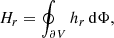
The appropriate magnetic helicity for the Sun is relative magnetic helicity (Berger & Field 1984). For a three-dimensional (3D) magnetic field B in a finite volume V, this is given by the Finn & Antonsen (1985) formula
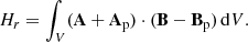
The magnetic field Bp serves as a reference field and it is usually chosen to be potential, while A, Ap are the respective vector potentials of the two magnetic fields. Relative magnetic helicity is independent of the chosen gauges of the two vector potentials as long as the normal components of the magnetic fields are the same on the boundary of the volume, ∂V. This condition can be written as
where n̂ denotes the outward-pointing unit normal on ∂V.
2.2.2. Energies
Although we are not interested in the evolution of the various energies in this work, there are energy-related parameters that help us identify the quality of a given magnetic field. We introduce these parameters in this section.
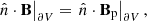
The energy of a magnetic field B is given by the well-known relation
where μ0 is the magnetic permeability of the vacuum. A useful decomposition of this energy is based on the unique splitting of the magnetic field into potential and current-carrying components, B = Bp + Bj. Following Valori et al. (2013), each component can be further divided into solenoidal and non-solenoidal parts, as Bp = Bp, s + Bp, ns and Bj = Bj, s + Bj, ns. By defining the energy of each component from Eq. (3) we end up with the following decomposition:

where Emix denotes the energy corresponding to all the cross terms. For a perfectly solenoidal magnetic field, Eq. (4) reduces to the more familiar form E = Ep, s + Ej, s, where Ej, s can be identified as the free energy.
The non-solenoidal parts of the magnetic fields and the respective terms in Eq. (4) are non-physical and stem solely from numerical errors. Collecting these terms together, leads to the definition of the energy as

which is a measure of how much a numerical model of a magnetic field deviates from solenoidality; lower values of Ediv, and consequently of the energy ratio Ediv/E, indicate a less solenoidal magnetic field. Regarding helicity computations, Valori et al. (2016) set a threshold of Ediv/E ≲ 0.08 for helicity values to be reliable, which is later refined to Ediv/E ≲ 0.05 by Thalmann et al. (2019a), where the various energies for the same AR 11158 are discussed.
Another energy ratio that is related to the quality of a magnetic field with respect to its solenoidality is |Emix|/Ej, s, which shows the importance of the cross term in Eq. (4) relative to the free energy. Values of |Emix|/Ej, s ≲ 0.35 are related with magnetic fields of higher quality (Thalmann et al. 2020).
2.2.3. Relative field line helicity
2.2.4. a. Unconstrained gauge
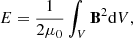
The most general expression for the FLH that corresponds to relative magnetic helicity was derived in Moraitis et al. (2019), and this expression is reviewed in this section for completeness. Relative field line helicity, hr, can be considered as the density of relative magnetic helicity per unit magnetic flux. This follows from the relation
where dΦ = |n̂ · B| dS is the elementary magnetic flux on the boundary (dS: elementary area). Equation (6) results directly from Eq. (1) after expanding the integrand of the latter and splitting the volume element along the field lines of B as dV = dS ⋅ dl, or, of Bp as dV = dS ⋅ dlp (dl, dlp: elementary lengths along respective field lines). The only assumption made in deriving Eq. (6) is the reasonable smoothness of the magnetic field, and especially the lack of null points where field lines are discontinuous. Additionally, this relation is useful when most of the field lines of B are connected to the boundary at both ends, that is when the number of closed field lines inside the volume is limited.
As its name indicates, RFLH is a function of the field lines that assigns a single value to each field line (pair of footpoints), and thus can be viewed as a 2D map that depends on the location on the boundary. Denoting the part of the boundary at which magnetic flux enters into (leaves) the volume as ∂V+ (∂V−), and the footpoints of a generic field line of B as α+ ∈ ∂V+, α− ∈ ∂V− (and as αp+ ∈ ∂V+, αp− ∈ ∂V− for Bp, respectively), then RFLH is given by any of the following expressions:
or
or, by their average, as
The first expression involves the integration along field lines of B and Bp that have common their positive-polarity footpoints, α+ = αp+, as shown by the red and green field lines in Fig. 1. When using  in Eq. (6), only the positive-polarity part of the boundary, ∂V+, should be considered, so that each field line is counted once.
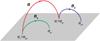 |
Fig. 1. Sketch of the field lines involved in the definition of RFLH. |
Similarly, if the field lines of the two fields have in common the negative-polarity footpoints, α− = αp−, then the RFLH expression given by Eq. (8) should be used along the ∂V− boundary (red and blue field lines in Fig. 1). When the whole boundary is considered, the respective RFLH, Eq. (9), involves all field lines shown in Fig. 1. In all cases the RFLH is expressed as a line integral along the field lines of B relative to the same quantity along those of Bp, thus justifying its name.
2.2.5. b. Berger and Field gauge
The expressions for RFLH given above make no assumption on the gauge of the vector potentials. RFLH however is a gauge-dependent quantity, as can easily be seen from any of Eqs. (7)–(9), and this can be exploited to derive simpler expressions for the RFLH. A commonly used gauge for the two vector potentials is given by the relation
This gauge condition can be fulfilled with the tangential components of Ap determined from those of A, while the latter can be in any gauge. The condition given by Eq. (10) leads to the elimination of the cross terms in the integrand of Eq. (1), which is written as
This gauge was used in the original definition of relative magnetic helicity by Berger & Field (1984). Starting from Eq. (11), Yeates & Page (2018) defined the following RFLH:
written here for the positive-polarity boundary, with analogous to Eqs. (8) and (9) relations holding for the other expressions,  ,
,  . These relative RFLHs are constructed similarly to the RFLHs in the unconstrained gauge, but they employ a specific gauge condition.
2.3. Implementation
2.3.1. Magnetic field modelling
All physical quantities that interest this work require as input the 3D magnetic field in the coronal volume. The 3D field at each instant is reconstructed from the corresponding observed HMI magnetogram with a NLFF method. This uses a weighted optimization approach (Wiegelmann & Inhester 2010), after pre-processing the horizontal components of the field on the photosphere so that it becomes more compatible with the force-free assumption, and additionally, smoothing of the original vector magnetogram. The full details of the method can be found in Thalmann et al. (2019b), where this reconstruction was first used.
We only mention in this work that the original HMI data were slightly cropped so that to leave quiet-Sun regions outside, and then rebinned by a factor of four, to the resolution of 2″ per pixel. The resulting NLFF field occupies the volume 215 Mm × 130 Mm × 185 Mm, and it is discretized by 148 × 92 × 128 grid points. In total, there are 115 snapshots with the typical cadence of 1 hr, except around the M6.6 and the X2.2 flares, when HMI’s highest cadence of 12 min was used.
The morphology of the extrapolated magnetic field for a snapshot ∼1 h before the X-class flare is shown in Fig. 2. A low-lying flux rope surrounded by an arcade field can be identified there, as is already known by other works (e.g., Sun et al. 2012; Nindos et al. 2012). Moreover, Fig. 2 shows that the RFLH values of the flux rope are higher than in the arcade field.
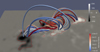 |
Fig. 2. Morphology of the 3D magnetic field of AR 11158 on 01:11 UT of 15 February 2011, for the NLFF extrapolation used in this work. The field lines are coloured according to the value of RFLH, which is positive for all selected field lines; they are overplotted on the photospheric distribution of the vertical magnetic field, with the red contours corresponding to the values |Bz| = 500 G. |
One of the reasons for choosing the specific AR for this study is the excellent quality of the reconstruction of the 3D magnetic field of the AR. The quality of the field is intended as the accuracy in fulfilling the assumptions of the NLFFF method, as quantified by the low values of divergence- and force-freeness reported in Thalmann et al. (2019b). The respective parameters used by the authors are the average absolute fractional flux increase and the average current-weighted angle between the current and magnetic field (Wheatland et al. 2000).
Besides these parameters the high level of divergence-freeness of the magnetic field is further shown with the following three parameters. The first is the recently proposed modification of the fractional flux increase which, unlike the original parameter, is independent of the mesh size (Gilchrist et al. 2020). This is very low, with a mean value over all the 115 snapshots of ⟨|fd|⟩ = (1.50 ± 0.06) × 10−9 m−1. Additionally, the energy ratio proposed by Valori et al. (2016) is well below the threshold of 0.08, or even of 0.05, with a value of Ediv/E = (6.1 ± 0.3) × 10−3. The other energy ratio (Thalmann et al. 2020) is also much lower than the respective limit of 0.35, with a value of |Emix|/Ej, s = 0.051 ± 0.006. Such high quality of the reconstructed magnetic field thus guarantees the reliability of the subsequent helicity computations.
2.3.2. Numerical computations
The computation of all the physical quantities can be performed in a three-step process once the magnetic field is provided by the NLFF method. The first step is the computation of the potential field that satisfies the condition of Eq. (2). This is derived by numerically solving Laplace’s equation. The second step involves the computation of the vector potentials from the respective magnetic fields. This is done by adopting the DeVore (2000) gauge as this was modified by Valori et al. (2012). The full details involved in these two steps are described in Moraitis et al. (2014).
The third step is required only for the RFLH computations and involves two different field line integrations: one for B and one for Bp. These integrations are performed with the fast and robust method that is described in Moraitis et al. (2019). A difference with that work is that here we consider only the field lines with (at least one) footpoint on the photospheric part of the boundary. We thus neglect the lateral and top parts of the boundary, as our experience has shown that a very small piece of information is lost. Once the field lines are obtained, we compute the RFLH expression in the unconstrained gauge,  , from Eq. (9).
For the computation of the RFLH in the Berger & Field gauge,  , the three-step process is slightly different than the process just described. This is because the computation is performed with the code provided by Yeates & Page (2018), which uses a different calculation for the potential magnetic field and treats all vector quantities in a staggered grid instead of being colocated.
3. Results
3.1. RFLH morphology
Following the methodology in Sect. 2 we calculate all quantities of interest for all available snapshots of the NLFF magnetic field model. In Fig. 3 we show four snapshots from the evolution of the morphology of RFLH on the photospheric plane (z = 0) in the unconstrained gauge,  ; of the vertical magnetic field, Bz; and of the vertical electrical current, jz = (∇×B)z/μ0, on the photospheric level as well. Each snapshot provides an example of the field configuration in each of the four intervals in which the major flares divide our study interval into: one before the M6.6 flare, one between the two M-class flares, one between the M2.2 and the X2.2 flares, and one after the X2.2 flare.
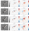 |
Fig. 3. Photospheric maps of vertical magnetic field, Bz (left), vertical electrical current, jz (middle), and RFLH (right) in AR 11158 for four snapshots during the studied interval. The red contours correspond to the vertical magnetic field values |Bz| = 500 G at each instant. |
The morphology of the vertical magnetic field evolved from two initial nearby bipoles that converged into a highly sheared bipolar flux distribution internal to the outer polarities (e.g., Chintzoglou & Zhang 2013). The vertical current distribution primarily develops around the polarity inversion lines (PILs) and follows, to a large degree, the evolution of the magnetic field, as the comparison with the respective contours shows in Fig. 3. The RFLH morphology is however different than the other distributions. The RFLH morphology is more extended and has a much less coincidence with the magnetic field contours. The sign of the RFLH is mostly positive, which agrees with the AR helicity sign. The highest (positive) RFLH values are located around the core polarities of the AR. This central part of RFLH becomes more intense until around the time of the X-class flare, and finally relaxes to lower values. The behaviour of RFLH around the flare is examined in more detail in Sect. 3.3. The lowest RFLH values are found to the east periphery of the AR (left in the respective panels of Fig. 3), with only a small coincidence with the nearby magnetic field polarity.
The corresponding evolution of the relative helicity budgets, as calculated by the volume method of Eq. (1), and of the RFLH method of Eq. (6) on the full magnetogram, is shown in Fig. 4 with the black and grey curves, respectively. We note that from 13 February onwards, the helicities obtained with the two methods agree to a large extent. We quantify this agreement in the bottom panel of Fig. 4, in which we note that the relative difference between the two curves is within ≲5%, with an average absolute value of 2.2%. In calculating these numbers, we omit the day of February 12 when the values of helicity are very low and consequently the relative difference is much higher than in the following days. The closeness of the two helicity curves indicates that the RFLH method works as expected, since it exhibits similar levels of agreement as in Moraitis et al. (2019). It also shows that most of the field lines contributing to helicity are rooted in the phothosphere rather than on the lateral boundaries. Both methods indicate a large drop in helicity during the X-class flare, which we further discuss in the following sections.
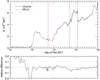 |
Fig. 4. Evolution of relative helicity in AR 11158 as calculated by the volume (Eq. (1), black line), and the RFLH methods (Eq. (6), grey line) in the top panel, and of their relative difference in the bottom, during the whole studied interval. The vertical lines denote the times of the two M- and of the X-class flares. |
We note that the morphology of RFLH is not sensitive to the gauge used in its computation, at least in areas of high RFLH values. This can be seen in Fig. 5 in which we compare the morphology obtained with the two gauges of Sect. 2 for the snapshot at 07:59 UT of 15 February 2011. We see that the two distributions have similar morphologies, although they also exhibit some minor differences in small patches. The good agreement of the two maps is depicted in the high value of the pixel-to-pixel linear correlation coefficient between them, which is 0.85. The main difference between the two distributions is in the magnitude of RFLH, which is by a factor of ≲2 smaller in the Berger & Field gauge. The morphology in this gauge is also more smooth because of the Coulomb gauge used in the computation of the vector potentials. Similar differences are exhibited in the other snapshots as well.
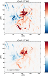 |
Fig. 5. Photospheric morphology of the RFLH in the unconstrained gauge (top) and in the Berger & Field gauge (bottom) for AR 11158 on 07:59 UT of 15 February 2011. The two images exhibit a pixel-to-pixel linear correlation coefficient of 0.85. |
3.2. Flare-related changes during the X2.2 flare
We now focus on the X2.2 flare of AR 11158 of 15 February 2011. The onset time of the flare was 01:44 UT and its peak time was 01:56 UT. Using observations from the SDO AIA instrument at 1600 Å, we are able to identify two regions related to the occurrence of the flare. The first is the location of the flare ribbons (shown in the top panel of Fig. 6) at the time of their maximum extent (01:48 UT) before the saturation of the image from the flare emission. According to the standard model for the 3D flares (Janvier et al. 2013), the flare ribbons correspond to the footprints of the quasi-separatrix layer (QSL), which separates the flux rope from the surrounding, confining field. This image resulted after correcting the original AIA image with standard methods (solar software’s aia_prep routine), and transforming it to the same projection and field of view (FOV) as the HMI images of Fig. 3, following the recipes of Sun (2013). The latter procedure slightly deforms the shape of the image, but this is minimal due to the proximity of the AR to the solar disc centre. We approximate the region corresponding to the central, highest intensity contour with the red polygon shown in the bottom panel of Fig. 6. The second region of interest includes the central polarities of the AR where the flare originated during its peak (as identified by eye inspection of the AIA images), although nearly the whole AR participated in this flare. This region is shown as a green box in the bottom panel of Fig. 6 and encompasses the area covered by the ribbons when they reach their maximum extent.
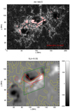 |
Fig. 6. AIA image at 1600 Å of the same AR region shown in Fig. 3 saturated at the intensity of 1180 and overplotted with the contours at the same value at the beginning of the X2.2 flare of AR 11158 (top). Zoom of the vertical magnetic field 2D map at the same time, with the two regions of interest (bottom). Red contours are the same as in the top panel, only rebinned to the resolution of the magnetic field image. Yellow contours correspond to the magnetic field value Bz = 0 G. |
In the panels a, b, d, and e of Fig. 7 we show the evolution of the RFLH distribution in the corresponding areas around the X-class flare. We note that the overall morphology has small variations in a two-hour interval around the flare. The most important difference is the large decrease in the RFLH magnitude between the snapshots at 01:47 UT and 01:59 UT, that is during the maximum of the flare. This is more evident in panels c and f, in which the difference of the images at 01:47 UT and at 01:59 UT with the image at 01:11 UT is shown, respectively. While the first difference image shows small variations of both signs in the whole FOV, the second image depicts a clear decrease in RFLH.
 |
Fig. 7. Selected snapshots of the zoomed-in photospheric morhology of RFLH around the X2.2 flare of AR 11158 (panels a, b, d, e). Also shown are the two boxes defined in Fig. 6 and the contours of the vertical magnetic field values at |Bz| = 500 G. Difference images of the photospheric RFLH at the beginning of the flare (at 01:47 UT, panel c) and after the flare (at 01:59, panel f) with respect to the corresponding pre-flare image at 01:11 UT. The boxes are the same as in the rest panels. |
The use of RFLH thus enables us to identify the locations where helicity is lost from the AR during the flare and the respective eruption; RFLH also allows us to calculate the value of the lost helicity. It is also interesting that the area of the RFLH decrease includes the location of the flux rope, and so we can deduce that a part of the flux rope was expelled during the flare. In other words, we are able to verify that the CME source coincides with the wider flux rope region. This conclusion agrees with many previous studies (e.g., Zhang et al. 2012; Patsourakos et al. 2013; Nindos et al. 2015, 2020; Chintzoglou et al. 2015).
In Fig. 8 we show the evolution of various helicity budgets around the X2.2 flare. The black and grey curves are a zoom-in around the time of the X2.2. flare of the same helicity budgets as calculated by the volume and the RFLH methods for the full magnetogram, shown in Fig. 4. We also show the errors stemming from the difference of the helicity curves from their five-point moving averages, which correspond to one-hour intervals. We use this type of error as an indication of the actual errors, since the computationally deduced errors by the method of Moraitis et al. (2014), are very low.
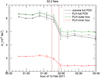 |
Fig. 8. Evolution of relative helicities in AR 11158 during a two-hour interval centred on the X2.2 flare. Shown are the relative helicities as calculated by the volume method (Eq. (1), black line), and by the RFLH method using Eq. (9) in the whole AR (grey line) and in the two boxes of Fig. 6 (red and green lines). The error bars are computed from the difference of the curves from their five-point moving averages. The vertical lines denote the onset and peak times of the X-class flare. |
In addition, Fig. 8 depicts the helicity budgets calculated by the RFLH method for the two boxes of Fig. 6. In calculating these, we employ Eq. (6) but consider only those field lines that have footpoints inside the respective areas.
Figure 8 reiterates the good agreement of ≲5% between the helicities obtained by the volume and the RFLH methods. Both curves exhibit a 25% drop in helicity during the flare, which corresponds to 1.48 1042 Mx2 for the volume method and to the slightly larger 1.56 1042 Mx2 for the RFLH method. The drop in the volume helicity is larger than the computed errors and so it is not an artefact but a real drop; this conclusion holds for the other helicity curves as well. Similar sharp changes in other parameters related to the magnetic field were reported previously for the same AR (Liu et al. 2012; Sun et al. 2017).
Another conclusion that can be drawn from Fig. 8 is that the helicities obtained by the RFLH method for the full FOV and for the green box agree to a large extent. This can be explained because the majority of the helicity of the AR is contained in the green box, a conclusion also supported by the RFLH morphology in Fig. 7. The agreement is more pronounced before the flare when the two curves agree to within 0.5%. After the flare however this falls to 5%, which should be attributed to the rearrangement of the magnetic field during the flare, and to a lesser extent, to the evolution of the arc-shaped RFLH structure just above the green box in Fig. 7. Finally, the drop in helicity coming from the green box is 20%, a bit less than in the full FOV and corresponds to a value of 1.35 1042 Mx2.
Focussing next to the red box that approximates the ribbons of the flare, we note that the helicity contained in it is the half of the entire AR. The relative drop in helicity during the flare is similar to the other curves, that is ∼22% of its pre-flare value; its absolute value however is much smaller, corresponding to 7.1 1041 Mx2. This small relative drop indicates that the region stays non-potential even after the expulsion of the flux rope. On the other hand, the higher (absolute) helicity drop within the green box suggests that the effect of the CME is to change the entire surrounding of the flux rope. An alternative explanation could be that the eruption changes the mutual helicity between the systems of the flux rope and the surrounding field, in which case the RFLH would reflect the non-local nature of helicity. This would also relate to the mutual-to-self conversion of helicity (Tziotziou et al. 2013), which was suggested for the same AR.
3.3. Relation with the eruption of February 15
The X2.2 flare of AR 11158 on February 15 was eruptive, that is it was accompanied by a CME. This was observed with the STEREO COR1 coronagraph at 2:05 UT of February 15 and had a peak velocity of ∼1300 km s−1 (Maričić et al. 2014). The ejected structure took a part of the helicity of the AR which, according to the previous section, should be positive (right-handed) and no more than the maximum estimated helicity decrease of ∼1.5 1042 Mx2. The CME was recorded three days later, starting at February 18 around 20:00 UT, as an interplanetary coronal mass ejection (ICME), using in situ data at the Lagrange point L1 from the Wind spacecraft (Maričić et al. 2014; Lepping et al. 2015). This ICME was also listed in several other catalogues (Richardson & Cane 2010; Chi et al. 2016; Hess & Zhang 2017) at a similar time interval.
From the fitting of the ICME with a linear force-free magnetic cloud (MC) model, Lepping et al. (2015, Table 2 therein) find a value for the axial magnetic field strength of B0 = 11.4 nT, and for the radius of the MC, r0 = 0.06 AU. If we further assume the arbitrary, but consistent (however with energetic electron recordings in ICMEs; Kahler et al. 2011), length for the MC of L ∼ 2 AU, we can estimate the helicity of the ICME to Hr ∼ 2 1041 Mx2 following the equations in Dasso et al. (2006). This value is significantly smaller than the entire helicity of the AR as well as of the helicity contained in the two boxes. The comparison with the corresponding helicity drops shows that the helicity of the MC is a factor of ∼7 smaller than the helicity lost from the whole AR or from the green box area. It is closer however to the helicity lost in the area of the flare ribbons, but still a factor of ∼3 smaller. A problem with the helicity reported in Lepping et al. (2015) is that this is left-handed, that is it has opposite sign compared to the AR. Moreover, as discussed by Lepping et al. (2015), the quality of the MC fitting for this ICME is poor, exhibiting convergence issues. Therefore, this ICME does not represent the most optimal case for comparisons with solar observations. Despite all the uncertainties in the estimation of the helicity of the MC, the absolute value obtained is consistent with the upper limit derived from the helicity drop in the whole AR.
4. Discussion
This work dealt with the first detailed study of RFLH in a solar AR. The target AR 11158 exhibited intense activity during the four-day study interval. The computation of RFLH was based on the relevant recent developments and on a high-quality NLFF model for the coronal magnetic field of the AR, thus ensuring reliable helicity estimations.
The examination of the photospheric morphology of RFLH showed that this is very different than the respective distributions of the magnetic field and the electrical current. Furthermore, the morphology of RFLH was shown not to be sensitive on the employed gauge in its computation. The total AR helicity as estimated by the RFLH agrees to a large extent with the more accurate, volume helicity method, as was already demonstrated before.
Our results are consistent with the picture drawn by other works on AR 11158, for example that of Jing et al. (2012). These authors find a similar helicity evolution, both overall and during the X-class flare. The helicity of the AR exhibited a sharp decrease during the X2.2 flare, ∼25% of its pre-flare value. A similar sharp drop was reported in Jing et al. (2012), which, moreover, resulted from the respective drop in the right-handed helicity. This is exactly what the RFLH photospheric maps of Sect. 3.2 reveal.
The main advantage of using RFLH is the additional spatial information that this method can provide about the locations where helicity is more important and its respective values. In the case of the X2.2 flare of AR 11158, we found that the decrease in helicity is coming mostly from the wider flux rope area. Additionally, by examining two observationally deduced, flare-related regions, we were able to monitor the individual helicity evolution in each of them. The helicity drop during the flare in these regions did not reveal a clear relation with the helicity of the observed ICME, although there are many uncertainties in the derivation of the latter.
As a conclusion, this work pointed out the usefulness of RFLH in solar applications. The spatial information provided by RFLH can help in situations such as that examined in this paper, that is in the determination of the pre-eruptive structures of CMEs. A possible next step in the study of RFLH would be to perform similar analysis to a number of ARs with different levels of activity and different characteristics, and juxtapose these with the helicity of the associated ICMEs at 1 AU or even much closer in the corona or inner heliosphere with Parker Solar Probe (Fox et al. 2016) and Solar Orbiter (Müller et al. 2020). This would enable the examination of the behaviour of RFLH in different environments and the possibility of discriminating solar activity with the help of RFLH.
Acknowledgments
The authors thank the referee for carefully reading the paper and providing constructive comments. This research is co-financed by Greece and the European Union (European Social Fund – ESF) through the Operational Programme “Human Resources Development, Education and Lifelong Learning” in the context of the project “Reinforcement of Postdoctoral Researchers – 2nd Cycle” (MIS-5033021), implemented by the State Scholarships Foundation (IKY). It also benefited from the discussions within the international team “Magnetic Helicity in Astrophysical Plasmas” which was supported by the International Space Science Institute. The authors also thank J. Thalmann for providing the NLFF reconstruction of the AR’s magnetic field.
References
- Aly, J.-J. 2018, Fluid Dyn. Res., 50, 011408 [NASA ADS] [CrossRef] [Google Scholar]
- Antiochos, S. K. 1987, ApJ, 312, 886 [NASA ADS] [CrossRef] [Google Scholar]
- Berger, M. A. 1988, A&A, 201, 355 [Google Scholar]
- Berger, M. A., & Field, G. B. 1984, J. Fluid. Mech., 147, 133 [Google Scholar]
- Chi, Y., Shen, C., Wang, Y., et al. 2016, Sol. Phys., 291, 2419 [NASA ADS] [CrossRef] [Google Scholar]
- Chintzoglou, G., & Zhang, J. 2013, ApJ, 764, L3 [NASA ADS] [CrossRef] [Google Scholar]
- Chintzoglou, G., Patsourakos, S., & Vourlidas, A. 2015, ApJ, 809, 34 [NASA ADS] [CrossRef] [Google Scholar]
- Dasso, S., Mandrini, C. H., Démoulin, P., & Luoni, M. L. 2006, A&A, 455, 349 [NASA ADS] [CrossRef] [EDP Sciences] [Google Scholar]
- DeVore, C. R. 2000, ApJ, 539, 944 [NASA ADS] [CrossRef] [Google Scholar]
- Finn, J., & Antonsen, T. 1985, Comm. Plasma Phys. Control. Fusion, 9, 111 [Google Scholar]
- Fox, N. J., Velli, M. C., Bale, S. D., et al. 2016, Space Sci. Rev., 204, 7 [NASA ADS] [CrossRef] [Google Scholar]
- Gilchrist, S. A., Leka, K. D., Barnes, G., Wheatland, M. S., & DeRosa, M. L. 2020, ApJ, 900, 136 [CrossRef] [Google Scholar]
- Green, L. M., Török, T., Vršnak, B., Manchester, W., & Veronig, A. 2018, Space Sci. Rev., 214, 46 [Google Scholar]
- Hess, P., & Zhang, J. 2017, Sol. Phys., 292, 80 [Google Scholar]
- Janvier, M., Aulanier, G., Pariat, E., & Démoulin, P. 2013, A&A, 555, A77 [NASA ADS] [CrossRef] [EDP Sciences] [Google Scholar]
- Jing, J., Park, S.-H., Liu, C., et al. 2012, ApJ, 752, L9 [NASA ADS] [CrossRef] [Google Scholar]
- Kahler, S. W., Krucker, S., & Szabo, A. 2011, J. Geophys. Res. (Space Phys.), 116, A01104 [Google Scholar]
- Lemen, J. R., Title, A. M., Akin, D. J., et al. 2012, Sol. Phys., 275, 17 [Google Scholar]
- Lepping, R. P., Wu, C. C., Berdichevsky, D. B., & Szabo, A. 2015, Sol. Phys., 290, 2265 [Google Scholar]
- Liu, C., Deng, N., Liu, R., et al. 2012, ApJ, 745, L4 [NASA ADS] [CrossRef] [Google Scholar]
- Low, B. C. 1994, Phys. Plasmas, 1, 1684 [NASA ADS] [CrossRef] [Google Scholar]
- Lowder, C., & Yeates, A. 2017, ApJ, 846, 106 [NASA ADS] [CrossRef] [Google Scholar]
- Maričić, D., Vršnak, B., Dumbović, M., et al. 2014, Sol. Phys., 289, 351 [Google Scholar]
- Moraitis, K., Tziotziou, K., Georgoulis, M. K., & Archontis, V. 2014, Sol. Phys., 289, 4453 [Google Scholar]
- Moraitis, K., Pariat, E., Valori, G., & Dalmasse, K. 2019, A&A, 624, A51 [NASA ADS] [CrossRef] [EDP Sciences] [Google Scholar]
- Müller, D., St. Cyr, O. C., Zouganelis, I., et al. 2020, A&A, 642, A1 [CrossRef] [EDP Sciences] [Google Scholar]
- Nindos, A., Patsourakos, S., & Wiegelmann, T. 2012, ApJ, 748, L6 [NASA ADS] [CrossRef] [Google Scholar]
- Nindos, A., Patsourakos, S., Vourlidas, A., & Tagikas, C. 2015, ApJ, 808, 117 [NASA ADS] [CrossRef] [Google Scholar]
- Nindos, A., Patsourakos, S., Vourlidas, A., Cheng, X., & Zhang, J. 2020, A&A, 642, A109 [CrossRef] [EDP Sciences] [Google Scholar]
- Pariat, É., Démoulin, P., & Berger, M. A. 2005, A&A, 439, 1191 [NASA ADS] [CrossRef] [EDP Sciences] [Google Scholar]
- Pariat, É., Valori, G., Démoulin, P., & Dalmasse, K. 2015, A&A, 580, A128 [NASA ADS] [CrossRef] [EDP Sciences] [Google Scholar]
- Patsourakos, S., Vourlidas, A., & Stenborg, G. 2013, ApJ, 764, 125 [NASA ADS] [CrossRef] [Google Scholar]
- Patsourakos, S., Vourlidas, A., Török, T., et al. 2020, Space Sci. Rev., 216, 131 [Google Scholar]
- Pesnell, W. D., Thompson, B. J., & Chamberlin, P. C. 2012, Sol. Phys., 275, 3 [Google Scholar]
- Richardson, I. G., & Cane, H. V. 2010, Sol. Phys., 264, 189 [Google Scholar]
- Russell, A. J. B., Yeates, A. R., Hornig, G., & Wilmot-Smith, A. L. 2015, Phys. Plasmas, 22, 032106 [NASA ADS] [CrossRef] [Google Scholar]
- Rust, D. M. 1994, Geophys. Res. Lett., 21, 241 [NASA ADS] [CrossRef] [Google Scholar]
- Scherrer, P. H., Schou, J., Bush, R. I., et al. 2012, Sol. Phys., 275, 207 [Google Scholar]
- Sun, X. 2013, ArXiv e-prints [arXiv:1309.2392] [Google Scholar]
- Sun, X., Hoeksema, J. T., Liu, Y., et al. 2012, ApJ, 748, 77 [NASA ADS] [CrossRef] [Google Scholar]
- Sun, X., Hoeksema, J. T., Liu, Y., Kazachenko, M., & Chen, R. 2017, ApJ, 839, 67 [Google Scholar]
- Taylor, J. B. 1974, Phys. Rev. Lett., 33, 1139 [NASA ADS] [CrossRef] [Google Scholar]
- Thalmann, J. K., Moraitis, K., Linan, L., et al. 2019a, ApJ, 887, 64 [Google Scholar]
- Thalmann, J. K., Linan, L., Pariat, E., & Valori, G. 2019b, ApJ, 880, L6 [NASA ADS] [CrossRef] [Google Scholar]
- Thalmann, J. K., Sun, X., Moraitis, K., & Gupta, M. 2020, A&A, 643, A153 [EDP Sciences] [Google Scholar]
- Tziotziou, K., Georgoulis, M. K., & Liu, Y. 2013, ApJ, 772, 115 [NASA ADS] [CrossRef] [Google Scholar]
- Valori, G., Démoulin, P., & Pariat, É. 2012, Sol. Phys., 278, 347 [NASA ADS] [CrossRef] [EDP Sciences] [Google Scholar]
- Valori, G., Démoulin, P., Pariat, É., & Masson, S. 2013, A&A, 553, A38 [NASA ADS] [CrossRef] [EDP Sciences] [Google Scholar]
- Valori, G., Pariat, É., Anfinogentov, S., et al. 2016, Space Sci. Rev., 201, 147 [NASA ADS] [CrossRef] [Google Scholar]
- Wheatland, M. S., Sturrock, P. A., & Roumeliotis, G. 2000, ApJ, 540, 1150 [Google Scholar]
- Wiegelmann, T., & Inhester, B. 2010, A&A, 516, A107 [NASA ADS] [CrossRef] [EDP Sciences] [Google Scholar]
- Woltjer, L. 1958, Proc. Nat. Acad. Sci., 44, 489 [Google Scholar]
- Yeates, A. R., & Hornig, G. 2016, A&A, 594, A98 [NASA ADS] [CrossRef] [EDP Sciences] [Google Scholar]
- Yeates, A. R., & Page, M. H. 2018, J. Plasma Phys., 84, 775840602 [CrossRef] [Google Scholar]
- Zhang, J., Cheng, X., & Ding, M.-D. 2012, Nat. Commun., 3, 747 [Google Scholar]
All Figures
|
Fig. 1. Sketch of the field lines involved in the definition of RFLH. |
| In the text | |
|
Fig. 2. Morphology of the 3D magnetic field of AR 11158 on 01:11 UT of 15 February 2011, for the NLFF extrapolation used in this work. The field lines are coloured according to the value of RFLH, which is positive for all selected field lines; they are overplotted on the photospheric distribution of the vertical magnetic field, with the red contours corresponding to the values |Bz| = 500 G. |
| In the text | |
|
Fig. 3. Photospheric maps of vertical magnetic field, Bz (left), vertical electrical current, jz (middle), and RFLH (right) in AR 11158 for four snapshots during the studied interval. The red contours correspond to the vertical magnetic field values |Bz| = 500 G at each instant. |
| In the text | |
|
Fig. 4. Evolution of relative helicity in AR 11158 as calculated by the volume (Eq. (1), black line), and the RFLH methods (Eq. (6), grey line) in the top panel, and of their relative difference in the bottom, during the whole studied interval. The vertical lines denote the times of the two M- and of the X-class flares. |
| In the text | |
|
Fig. 5. Photospheric morphology of the RFLH in the unconstrained gauge (top) and in the Berger & Field gauge (bottom) for AR 11158 on 07:59 UT of 15 February 2011. The two images exhibit a pixel-to-pixel linear correlation coefficient of 0.85. |
| In the text | |
|
Fig. 6. AIA image at 1600 Å of the same AR region shown in Fig. 3 saturated at the intensity of 1180 and overplotted with the contours at the same value at the beginning of the X2.2 flare of AR 11158 (top). Zoom of the vertical magnetic field 2D map at the same time, with the two regions of interest (bottom). Red contours are the same as in the top panel, only rebinned to the resolution of the magnetic field image. Yellow contours correspond to the magnetic field value Bz = 0 G. |
| In the text | |
|
Fig. 7. Selected snapshots of the zoomed-in photospheric morhology of RFLH around the X2.2 flare of AR 11158 (panels a, b, d, e). Also shown are the two boxes defined in Fig. 6 and the contours of the vertical magnetic field values at |Bz| = 500 G. Difference images of the photospheric RFLH at the beginning of the flare (at 01:47 UT, panel c) and after the flare (at 01:59, panel f) with respect to the corresponding pre-flare image at 01:11 UT. The boxes are the same as in the rest panels. |
| In the text | |
|
Fig. 8. Evolution of relative helicities in AR 11158 during a two-hour interval centred on the X2.2 flare. Shown are the relative helicities as calculated by the volume method (Eq. (1), black line), and by the RFLH method using Eq. (9) in the whole AR (grey line) and in the two boxes of Fig. 6 (red and green lines). The error bars are computed from the difference of the curves from their five-point moving averages. The vertical lines denote the onset and peak times of the X-class flare. |
| In the text | |
Current usage metrics show cumulative count of Article Views (full-text article views including HTML views, PDF and ePub downloads, according to the available data) and Abstracts Views on Vision4Press platform.
Data correspond to usage on the plateform after 2015. The current usage metrics is available 48-96 hours after online publication and is updated daily on week days.
Initial download of the metrics may take a while.