| Issue |
A&A
Volume 649, May 2021
|
|
|---|---|---|
| Article Number | A22 | |
| Number of page(s) | 14 | |
| Section | Catalogs and data | |
| DOI | https://doi.org/10.1051/0004-6361/202140310 | |
| Published online | 03 May 2021 | |
The ASTRODEEP-GS43 catalogue: New photometry and redshifts for the CANDELS GOODS-South field⋆
1
INAF – OAR, Via Frascati 33, 00078 Monte Porzio Catone, Roma, Italy
e-mail: This email address is being protected from spambots. You need JavaScript enabled to view it.
2
Las Campanas Observatory, Carnegie Observatories, Colina El Pino, Casilla 601, La Serena, Chile
3
Department of Physics, University of Oxford, Keble Road, Oxford OX1 3RH, UK
4
Instituto de Astrofísica e Ciências do Espaço, Universidade de Lisboa, Lisboa, Portugal
5
Laboratoire AIM-Paris-Saclay, CEA/DRF/Irfu – CNRS – Université Paris Diderot, CEA-Saclay, Pt Courrier 131, 91191 Gif-sur-Yvette, France
6
Institute for Astronomy, University of Edinburgh, Royal Observatory, Edinburgh EH9 3HJ, UK
7
INAF-Osservatorio Astronomico di Padova, Vicolo dell’Osservatorio 5, 35122 Padova, Italy
8
INAF – Osservatorio Astronomico di Trieste, Via Tiepolo 11, 34131 Trieste, Italy
9
Cosmic Dawn Center (DAWN); Niels Bohr Institute, University of Copenhagen, Lyngbyvej 2, 2100 Copenhagen, Denmark
10
Université de Strasbourg, CNRS, Observatoire Astronomique de Strasbourg, Strasbourg 67000, France
11
Space Telescope Science Institute, 3700 San Martin Drive, Baltimore, MD 21218, USA
Received:
11
January
2021
Accepted:
12
March
2021
Abstract
Context. We present ASTRODEEP-GS43, a new multi-wavelength photometric catalogue of the GOODS-South field, which builds and improves upon the previously released CANDELS catalogue.
Aims. We provide photometric fluxes and corresponding uncertainties in 43 optical and infrared bands (25 wide and 18 medium filters), as well as the photometric redshifts and physical properties of the 34930 CANDELS H-detected objects, plus an additional sample of 178 H-dropout sources, of which 173 are Ks-detected and five are IRAC-detected.
Methods. We keep the CANDELS photometry in seven bands (CTIO U, Hubble Space Telescope WFC3, and ISAAC-K) and measure from scratch the fluxes in the other 36 (23 from Subaru SuprimeCAM and Magellan Baade FourStar and the rest from VIMOS, HST ACS, HAWK-I Ks, and Spitzer IRAC) with state-of-the-art template-fitting techniques. We then compute new photometric redshifts with three different software tools and take the median value as a best estimate. We finally evaluate new physical parameters from spectral energy distribution (SED) fitting, comparing them to previously published ones.
Results. Comparing to a sample of 3931 high quality spectroscopic redshifts, for the new photometric redshifts we obtain a normalised median absolute deviation of 0.015, with 3.01% of outliers on the full catalogue (0.011 and 0.22% on the bright end at I814 < 22.5). This is similar to the best available published samples of photometric redshifts, such as the COSMOS UltraVISTA catalogue.
Conclusions. The ASTRODEEP-GS43 results are in qualitative agreement with previously published catalogues of the GOODS-South field, improving on them particularly in terms of SED sampling and photometric redshift estimates. The catalogue is available for download from the ASTRODEEP website.
Key words: techniques: photometric / catalogs / galaxies: fundamental parameters / galaxies: photometry / galaxies: distances and redshifts / methods: data analysis
A copy of the catalogue is only available at the CDS via anonymous ftp to cdsarc.u-strasbg.fr (130.79.128.5) or via http://cdsarc.u-strasbg.fr/viz-bin/cat/J/A+A/649/A22
© ESO 2021
1. Introduction
Multi-wavelength extragalactic astronomy targeting the high-redshift Universe has matured to the status of precision science over the past decade. Deep optical and infrared photometric surveys such as CANDELS (Grogin et al. 2011; Koekemoer et al. 2011), 3D-HST (Skelton et al. 2014) and Frontier Fields (Lotz et al. 2014; Koekemoer et al. 2014; Merlin et al. 2016b; Castellano et al. 2016; Shipley et al. 2018) have provided high quality multi-band imaging of various regions of the sky, combining data from space observatories (the Hubble and Spitzer space telescopes) with data from ground-based facilities (ESO Very Large Telescope, Keck, and Subaru), overcoming the spectroscopic limit and allowing for the analysis of statistically significant samples of galaxies up to z ∼ 8−9. These projects paved the way for the upcoming generation of observational campaigns and instruments, including large-scale surveys and deep imaging programmes (with the Vera Rubin Observatory/LSST and the Euclid, James Webb, and Nancy Grace Roman space telescopes) or the extremely high resolution power provided by adaptive optics (e.g. the Extremely Large Telescope MICADO instrument). The advent of such new facilities will further push the limits of our observations towards the earliest epochs of structure formation. As we await such exciting game changing technologies, there is still room to exploit the currently available data by combining all the archival observations to extract as much information as possible.
The CANDELS legacy stands among the most informative collections of extragalactic data. In particular, the Great Observatories Origins Deep Survey Field South (GOODS-South) represents a benchmark for its exquisite quality and its richness. Located at RA = 3h 32m 30s, Dec = −27° 48m 20s, with an area of ∼173 sq. arcmin, GOODS-South has been observed by a number of observatories, both from the ground and from space, at all wavelengths from X-rays to radio (e.g. Elbaz et al. 2011; Ashby et al. 2013; Luo et al. 2017; Franco et al. 2018). It is worth mentioning here that the field will be the target of the James Webb GTO programme JADES (principal investigators Rieke and Ferruit). The official first generation CANDELS catalogue by Guo et al. (2013, hereafter G13) includes 34930 galaxies with photometric data in 17 wide passbands, from the ultraviolet (UV) to the mid-infrared, adding (then) new observations from HST WFC3 to existing archival images: nine HST bands (from the ACS and WFC3 cameras), four IRAC bands from Spitzer, three VLT bands (VIMOS U, ISAAC K, and HAWK-I Ks), and an additional U band from the CTIO MOSAIC instrument. The detection was performed on the WFC3 H160 band, using SEXTRACTOR (Bertin & Arnouts 1996) in a dual ‘hot+cold’ mode (Galametz et al. 2013); photometric measurements were performed using, again, SEXTRACTOR on the HST images to measure the total magnitude on the detection band and to measure point spread function (PSF) matched isophotal colours for the other bands; conversely, a template-fitting technique was used to directly estimate total fluxes on ground-based and IRAC images with the code T-FIT (Laidler et al. 2007). The 3D-HST catalogue by Skelton et al. (2014) also used part of this first collection of data.
Subsequently, two additional bands (VIMOS B and WFC3 J140) and deeper Ks photometry from HAWK-I (HUGS survey; Fontana et al. 2014; Grazian et al. 2015) were added to the archival data, and new HST-ACS deep mosaics were released by the Hubble Legacy Fields (HLF) project1 (Illingworth et al. 2016; Whitaker et al. 2019). Furthermore, deeper mosaics on 3.6 and 4.5 μm IRAC channels (CH1 and CH2) were created by R. McLure and used by Merlin et al. (2018, 2019), although no catalogue was released for these images.
This new generation of data, gathered since 2013, along with the introduction of new techniques and software such as T-PHOT (Merlin et al. 2015, 2016a), sparked the necessity of reviewing the original catalogue. In this paper we present ASTRODEEP-GS43, a new photometric and photo-z catalogue for GOODS-South that is intended to yield a comprehensive set of optical and near-infrared photometric information on the field, ahead of the advent of the upcoming next-generation datasets that will result from new instruments. This release builds on the previously published CANDELS catalogue and complements similar recently published efforts, such as the 3D-HST catalogue by Skelton et al. (2014) and the HLF catalogue by Whitaker et al. (2019).
We summarise here the main improvements with respect to the previous CANDELS catalogue. We kept the G13 detection list on the WFC3 H160 band. However, we added photometric measurements on 18 Subaru SuprimeCAM medium bands (Cardamone et al. 2010, MUSYC catalogue), five medium bands from Magellan Baade FourStar (Straatman et al. 2016, ZFOURGE survey), and the B and R bands from VIMOS to the 18 previously released wide bands; as such, the total number of passbands is now 43. They are described in Sect. 2.
Additionally, we added 173 new objects detected in the HUGS HAWK-I Ks image, as described in Sect. 3.1, to the catalogue. We also added five additional sources detected in the Spitzer IRAC CH1 and CH2 bands. Of the sources detected in the latter bands, three are from the list of ten H-dropouts by Wang et al. (2016, hereafter W16); the remaining seven from their list were already included in our list of Ks detections. The final two IRAC-detected sources were again found by Wang and Collaborators (priv. comm.), but they had been excluded from their published list (see Sect. 3.2).
Thirdly, we measured HST ACS fluxes from the new, deep mosaics released by the HLF project, again using SEXTRACTOR to extract isophotal aperture PSF-matched photometry. We point out that the latest HLF data release (v2.0) includes photometric data on UV bands; however, when we compiled our catalogue, the latest available release was v1.5, which did not include UV images. For this reason, ASTRODEEP-GS43 does not include UV data. We do not consider this a major drawback since the main focus of the present release is on high-redshift galaxies, for which UV observations are not crucial.
Finally, we exploited the template-fitting code T-PHOT v2.0 to extract new photometry from the images of ground-based medium bands and Spitzer bands using three substantial algorithmic improvements with respect to the standard methods of v1.0: (i) the use of priors from the closest-wavelength high-resolution band for all the medium bands, as opposed to only priors from the H-detection band, (ii) background subtraction during the fitting process and (iii) individual locally variable PSFs for IRAC (these techniques are presented in Merlin et al. 2016a, and are summarised in Sect. 4). Also, two of the IRAC images (CH1 and CH2) are the new mosaics, which are deeper than those used for the CANDELS release; as such, we gain a substantial amount of detections that had previously been catalogued as upper limits.
This paper is structured as follows. In Sect. 2 we describe the full dataset. In Sect. 3 we focus on the detection techniques adopted to single out H-band dropouts on the Ks-band image. In Sect. 4 we discuss the photometric methods adopted on the new images, particularly on the medium bands. In Sect. 5 we present the new estimated photometric redshifts and physical properties, also comparing our results to previous ones and showing some diagnostic plots. Finally, in Sect. 6 we summarise the work and discuss some conclusions and possible future developments. Throughout the paper we adopt AB magnitudes (Oke & Gunn 1983) and standard cosmological parameters (H0 = 70.0 km s−1 Mpc−1, ΩΛ = 0.7, and Ωm = 0.3).
2. Dataset
The catalogue includes photometric data on 43 bands, which we describe in this section. The full list of the filters is given in Fig. 1 and Tables 1 and 2, with data taken from the SVO Filter Service Profile website (Rodrigo et al. 2012)2.
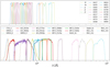 |
Fig. 1. Complete passband set for the ASTRODEEP-GS43 catalogue. Upper panel: filters of the SUPRIMECAM and FOURSTAR bands, while the lower panel: wide bands from HST, Spitzer, and ground-based facilities; the curves are normalised to arbitrary units to make them peak at unitary transmission. |
Summary of the 20 wide bands in the catalogue.
Summary of the 23 ground-based medium bands in the catalogue.
2.1. HST bands
We included ten bands from HST: five from ACS (F435W, F606W, F775W, F814W, and F850LP) and five from WFC3 (F098M, F105W, F125W, F140W, and F160W). As already mentioned, the ACS images are the new mosaics released by the HLF project (v1.5), in which all publicly available HST observations on the Chandra Deep Field South region have been added to the archival CANDELS images. The improvement with respect to CANDELS ACS mosaics is particularly significant in the I814 band, where the exposure time per pixel is increased by a factor of ≳2−3, depending on position. The WFC3 images are the same as those used for the official CANDELS survey catalogue of GOODS-South by G13. Full details on data processing and mosaic preparation are provided in Illingworth et al. (2016) and Whitaker et al. (2019) for the ACS bands, and in Koekemoer et al. (2011) for the WFC3 bands.
2.2. VLT
The catalogue includes the three VLT VIMOS bands: U, B, and R (Nonino et al. 2009). The U band was already included in the original CANDELS catalogue; however, we re-measured the fluxes on it using T-PHOT. On the contrary, the B and R band data had never been included in previous catalogues.
2.3. Subaru SuprimeCAM and Magellan FourStar bands
One of the most important additions to this release is the photometric measurements for 18 medium bands (typical width 20−30 nm) from the Subaru SuprimeCAM (Cardamone et al. 2010) dataset. We also included new measurements on the five Magellan Baade FourStar bands (Straatman et al. 2016). We stress that we did not directly include any previously published photometric measurements in our catalogue; rather, we used T-PHOT to obtain consistent and homogeneous photometry across the whole spectrum (see Sect. 4).
2.4. Spitzer
We used the IRAC CH1 and CH2 deep mosaics made by R. McLure (priv. comm.), obtained by combining images from seven observational programmes (one each by Dickinson, van Dokkum, Labbé, and Bouwens, and three by Fazio, including SEDS and S-CANDELS; see Ashby et al. 2015, for details) into two ‘supermaps’; they are equivalent to the ones by Labbé et al. (2015) and reach an average depth of ∼25.6 (total magnitude at 5σ) on both channels. On the other hand, CH3 and CH4 are the same mosaics used for G13. We used T-PHOT on all the IRAC bands; the photometric measurements on these mosaics have already been used in our recent work on passive galaxies in the early Universe (Merlin et al. 2018, 2019).
3. Detection of H-dropouts
We kept the G13 H-band list of 34930 sources as a baseline for our catalogue; the reader can find the details about the detection process in the original paper. On top of that, we added 173 sources detected on the deep HAWK-I Ks band (IDs from 34931 to 35103); we describe the detection method in the following subsection. Finally, we added five IRAC-detected sources (IDs from 35104 on) from the W16 study (see Sect. 3.2 for details). In total, we therefore have 35108 catalogued objects.
3.1. K-selected sources
We used two different approaches to detect sources on the Ks image, while excluding entries already present in G13.
Method 1 – Source Extractor in dual mode and cross-matching with G13. This method is aimed at detecting isolated sources that have escaped detection in the H band, typically because they are too faint (below the 5σ level), but are visible in K. We resampled the HUGS HAWK-I image (original pixel scale 0.1065″) to the HST mosaic pixel scale (0.06″) using SWARP (Bertin et al. 2002), and we degraded the H band to the K-band full width at half maximum (FWHM) of 0.43″. We then ran SEXTRACTOR in dual mode on the two images to detect and measure all sources in the Ks band and measure their flux in the H160 band (the parameters were optimised to favour the detection of low surface brightness or extended sources). We finally selected the objects with signal-to-noise ratios (S/N) higher than 5 that were not already present in G13 by means of a cross-correlation with a 1″ search radius (roughly equivalent to five H FWHMs, a conservative choice to avoid the risk of including dubious sources). With this procedure, we singled out 184 potential new sources (among these, five are not visible at all in the H band (< 1σ) and 130 are below the 5σ limit of G13; the remaining 49 are low surface brightness sources).
Method 2 – K-band residual image with T-PHOT. While Method 1 is tailored to detect isolated sources, it may fail to detect those that are close to the known H-detected sources because of the rejection within 1″. For such objects we exploited a second, complementary approach, using the residual image generated by T-PHOT when used to fit the Ks image with H-band priors: The sources that are not included in the H-band detection list, and therefore have not been fitted, appear as bright spots. However, we must take into account the fact that bright extended sources typically create irregular residuals, with negative and positive areas that could be mistaken for real sources by a detection algorithm. To cope with this, we created an enhanced rms map by summing the collage of the fitting models outputted by T-PHOT as a diagnostic image to the original rms of the Ks image; this map was then fed to SEXTRACTOR for the detection run, thus attributing a lower weight to areas occupied by known H-detected sources. We found that this simple technique yielded better results than using the original rms map, considerably reducing false positives – although it may also cause the exclusion of a few potentially true objects very close to bright H-detected sources, for which it would be difficult to obtain reliable photometric measurements anyway.
With this method we detected 267 sources, of which 170 had S/NK > 5; 82 of these 170 were also detected with Method 1. Apart from some spurious detections close to the borders of the image, and despite the effect of the weighting mask, we still found many detections clustered around very bright sources, which must be considered as false positives as well.
To compile the final list of K-selected sources we reviewed all the new candidates with S/NK > 5σ (that is, the 184 obtained through Method 1 plus the 170−82 = 88 additional ones obtained through Method 2), and we considered as valid sources only those that were visible by eye inspection in multiple bands (i.e. Ks plus IRAC and/or some HST band), or which had at least a very solid detection in the Ks band (i.e. non-spurious with high confidence). Via this process, after rejecting 99 sources based on our visual inspection, we finally obtained a total of 173 K-selected candidates: 75 are detected with both methods, 60 with Method 1 only, and 38 with Method 2 only. A few examples are shown in Fig. 2.
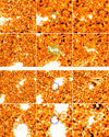 |
Fig. 2. Examples of new K-detected sources. Left to right: WFC3 H160, HAWK-I Ks, and T-PHOT residual on Ks. Upper panels (cyan circles): examples of sources detected with Method 1 (SEXTRACTOR in dual mode and cross-matching with G13). Lower panels (blue circles): examples of sources detected with Method 2 (K-band residual image with T-PHOT). See the text for details. |
3.2. IRAC-detected sources
Finally, we included a list of five IRAC-detected sources in ASTRODEEP-GS43. We started from the list of ten H-dropouts singled out by W1; in brief, they used the Ashby et al. (2013) 3.6 and 4.5 μm catalogue for the SEDS survey and selected H-dropouts by means of a cross-correlation with G13, excluding those with an H-band counterpart within 2″ (see the original paper for more details). Cross-correlating the coordinates, we found that seven out of the ten W16 galaxies were already present in our list of Ks-detected sources; therefore, only the remaining three W16 objects were added to our catalogue. Furthermore, we also included two more galaxies that were found by Wang and Collaborators in the same study (priv. comm.) but excluded from their final published list due to proximity with H-detected contaminants. Since their method was quite conservative and visual inspection ensured that the two sources are real H-dropouts, we decided to include them in our catalogue.
4. Photometry
We kept the photometric measurements from G13 for the five HST WFC3 bands. On the contrary, we measured photometry on the new HST ACS mosaics, with the same procedure adopted in G13 (see also Galametz et al. 2013). We used accurate PSFs from bright, unsaturated stars to build matching kernels between each band and the detection band H160, which has the widest FWHM. Isophotal fluxes were then measured on each PSF-matched ACS image using SEXTRACTOR in dual-image mode. The total fluxes were then obtained by correcting the detection band Kron flux (i.e. SEXTRACTORMAG_AUTO in H160) with a colour term computed as the ratio between the ACS and H160 isophotal fluxes.
We used the template-fitting software T-PHOT (Merlin et al. 2015, 2016a) on all the ground-based images, including the newly added medium bands. In brief, the code exploits stamps cut from high-resolution images as priors to build low-resolution templates; the latter are then used to minimise the difference between a model created as a collage of the templates and the real low-resolution image. All of the fits were performed using the entire image at once to ensure that the contamination from neighbours was taken into account. Rather than just using priors built only from the H-band image (as in the standard practice for K and Spitzer bands), for each measurement band we took as priors the cutouts from the closest HST band in terms of wavelength, provided the S/N of the object was higher than 3 in that band (if not, we reverted to the H-band prior). We verified that we obtained cleaner residuals with this approach.
Finally, we also used T-PHOT to measure photometry on all Spitzer bands (in this case using H-band priors). For these runs, we took advantage of three options of the v2.0 of the code: (i) each source was fitted with an individual convolution kernel obtained from the local PSF. We built each individual PSF by stacking instrumental PSF stamps, rotated according to the position angle of each single-epoch observation and weighted by its exposure time; (ii) a constant background was fitted and subtracted during the fitting process, along with the individual source fitting; (iii) individual positional registration of the sources was performed after a first fit to account for astrometric inaccuracies, re-centring the templates to minimise any spurious offset during a second fitting run. These techniques are described in detail in Merlin et al. (2016b). A visual depiction of the improvements obtained by using them is shown in Fig. 3.
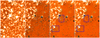 |
Fig. 3. From left to right: portion of the IRAC 3.6 μm mosaic by R. McLure; residuals after T-PHOT standard fitting using a single convolution kernel; residuals after fitting using a different individual kernel for each source, tailored on the basis of the positional angles of the pointings used to build the mosaic and with the T-PHOT global background subtraction option switched on; residuals for the final run, where the T-PHOT individual kernel registration option is also switched on (in the last two panels, blue boxes highlight regions where the improvement using this technique is evident). See the text for more details on the methods. |
Concerning the additional 173 K-detected sources, we processed all available HST bands using the same technique adopted for the H-detected sources, that is, smoothing them to the widest FWHM, in this case that of the Ks band. We then ran SEXTRACTOR in dual mode using the K-band image as the detection image for the 135 (60 plus 75) sources detected with Method 1, and the T-PHOT residuals in the Ks band for the remaining 38 sources detected with Method 2. In this case, considering the faintness of the sources, to obtain the total flux in each band we calculated the colour between the measurement band and Ks in a circular aperture of two FWHMs (a good compromise to avoid strong contamination while retaining the largest fraction of flux; see e.g. Castellano et al. 2010) and applied it to the K-band total flux.
The IRAC photometry was again obtained with T-PHOT; since the sources are typically small and faint, we adopted the PSF-fitting option, directly using the IRAC PSFs as priors rather than exploiting high-resolution cutouts. The same approach was used for the additional five IRAC-detected sources.
The final fluxes are consistent with the previously published ones, within the limits of the different methods used. The figures in Appendix A show quantitative comparisons of the new photometric measurements used in this work with the previous available ones in a number of reference bandpasses. Overall, the agreement is always reasonable, but many second-order differences can be spotted. In particular, it is already known that the 3D-HST fluxes differ from the that of CANDELS (e.g. Skelton et al. 2014; Stefanon et al. 2017), and they also retain this bias when compared to our new photometry. We did not investigate the reasons for such discrepancies.
5. Redshifts and physical properties
In this section we describe how we obtained the estimates of the photometric redshifts and of the main physical parameters, via spectral energy distribution (SED) fitting, for all the non-spectroscopic G13 H-detected sources and for the additional 178 K- and IRAC-detected ones. We note that the released catalogue lists the ‘best’ redshift estimate, which is the spectroscopic one whenever available and of good quality, and the photometric one otherwise.
5.1. Available spectroscopic data
First of all, we compiled a list of 4951 high quality and publicly available spectroscopic redshifts (of which 4829 are of galaxies and 122 are of stars) from a number of surveys and references (the full list is included in the catalogue README file). When two or more measurements were available for the same object, the one with the highest quality assigned flag was kept. We then used the spectroscopic redshifts to optimise the calibration of photometric redshifts, as described in Sects. 5.3.1 and 5.3.2. We point out that the list used in this procedure includes the VANDELS DR3, that was available at the time of submission; however, during the revision of this work the final DR4 became available (Garilli et al. 2021). After checking that differences were not substantial, we did not repeat the optimisation procedure, but we instead used the DR4 in the final Z-PHOT runs to determine the physical properties of the sources (Sect. 5.5), as well as in the published catalogue.
5.2. Star-galaxy separation
Before proceeding to estimate the photometric redshift and physical parameters of the catalogued galaxies, we cleaned the list of detected sources, flagging out those that can be safely identified as stars. First of all, we singled out and removed the spectroscopic sources; then we proceeded as in Grazian et al. (2007), combining the CLASS_STAR estimator (outputted by SEXTRACTOR from the original G13 detection run on the H band) with the analysis of the BzK diagnostic plane (Daddi et al. 2004), which we performed exploiting our new photometry from B435, Z850, and Hawk-I Ks. First, we selected the objects brighter than H = 24.5 (this is a conservative cut, but given that fainter magnitudes are prone to large photometric errors, and that in the low brightness regime high-redshift galaxies dominate over faint stars, we preferred the risk of wrongly classifying a real star as a galaxy rather than excluding real galaxies by misjudging them as stars). Then, among this selection, we flagged as stars the objects that both have CLASS_STAR > 0.85 and satisfy the BzK selection criterion, (z − K)< 0.3 × (B − z)−0.5. Combining the spectroscopic list with that obtained with this technique, we ended up with a final list of 174 stars; we included them in the catalogue but not in the subsequent analysis.
5.3. H-detected galaxies
To obtain photometric redshifts for the H-detected sources in G13 that do not have a spectroscopic observation, we exploited independent estimates from three SED-fitting software tools fed with the new photometric catalogue, namely LEPHARE (Arnouts et al. 1999; Ilbert et al. 2006), EAZY (Brammer et al. 2008), and ZPHOT (Fontana et al. 2000). We ran EAZY and ZPHOT on our local machines, while LEPHARE was run remotely via the GAZPAR web portal3.
For LEPHARE we used the same setting and parameters used in Ilbert et al. (2009) for their COSMOS catalogue. They include templates by Polletta et al. (2007) and additional starburst templates generated using BC03.
For the EAZY runs we used the built-in set of templates described in Sect. 2.2 of Brammer et al. (2008); we did not apply the Bayesian prioring option because, testing the possible configurations with a preliminary photo-z versus spec-z comparison, we found that including the priors yielded very similar results in terms of absolute dispersion, but also a slightly larger number of outliers, in particular a few objects at 1 < zspec < 3 wrongly estimated to have z ≃ 0. Given that the priors tend to disfavour high-redshift solutions, which in turn should be the most likely ones in deep surveys such as CANDELS, we preferred to proceed without them.
Finally, for the ZPHOT runs we compiled a library with two star formation histories (SFHs): a standard exponentially declining ‘τ model’ in which the star formation rate (SFR) is SFR(t) ∝ exp[−(t − t0)/τ] (where t0 is the beginning of the star formation activity); and a ‘delayed-τ’ SFH for which SFR(t) ∝ (t2/τ) × exp[−(t − t0)/τ]. We used Bruzual & Charlot (2003, BC03) templates that include nebular emission lines following Castellano et al. (2014) and Schaerer & de Barros (2009), assuming a Salpeter (1959) initial mass function (IMF) with a standard range of metallicities (0.02, 0.2, 1, and 2.5 Z/Z⊙, depending on the age of the models) and of dust extinctions (according to the Calzetti et al. 2000, law).
5.3.1. Zero-point corrections
For each of the three runs with different codes, we computed and applied independent zero-point corrections to the measured fluxes to obtain better final redshift estimates. We determined the corrections as follows. First, we made a run on the original photometric catalogue, after having cleaned it to remove unreliable entries (i.e. magnitudes and upper limits outside fiducial ranges, which, after a number of trials, we respectively set to [15,28] and 27 for all ground-based bands, [15,30] and 28 for HST bands, and [15,27] and 26 for IRAC). Then, we verified the output against a sub-selection of 3931 sources from the full spectroscopic sample described in Sect. 5.1 in the following way: We excluded from the full sample the sources that had a covariance index > 1 in one or more T-PHOT runs (because their photometry is unreliable due to dramatic blending) or had already been identified as active galactic nuclei (AGNs) by Cappelluti et al. (2016) or the VANDELS DR2 (Pentericci et al. 2018; McLure et al. 2018)4; also, we excluded sources whose photometric redshift fit had ![Mathematical equation: $ \chi^2=\sum [(f_{\rm meas}-f_{\rm model})^2/\sigma_{\rm meas}^2] > 500 $](/articles/aa/full_html/2021/05/aa40310-21/aa40310-21-eq1.gif) (we found via trials that this threshold is a good compromise to have robust results while keeping as many spectroscopic sources as possible). We used this reduced spectroscopic sample to compute zero-point corrections for each band: In practice, we ran the photometric codes once per band, keeping the redshift fixed at the spectroscopic value and ignoring the considered band in the fit, so that the flux of the best-fit model in that band is not affected by its observed value; the median of the difference between the observed magnitudes and the model magnitudes for all the objects gives the correction for the considered band. We then performed a second run using the zero-point corrected catalogue5. For most of the bands, the resulting corrections have absolute values below ∼0.05 mag; for a few exceptions they range from −0.15 (Subaru I827) to +0.25 (IRAC CH4) mag. This procedure led to a small but consistent improvement in the final statistics of the photometric versus spectroscopic comparison.
(we found via trials that this threshold is a good compromise to have robust results while keeping as many spectroscopic sources as possible). We used this reduced spectroscopic sample to compute zero-point corrections for each band: In practice, we ran the photometric codes once per band, keeping the redshift fixed at the spectroscopic value and ignoring the considered band in the fit, so that the flux of the best-fit model in that band is not affected by its observed value; the median of the difference between the observed magnitudes and the model magnitudes for all the objects gives the correction for the considered band. We then performed a second run using the zero-point corrected catalogue5. For most of the bands, the resulting corrections have absolute values below ∼0.05 mag; for a few exceptions they range from −0.15 (Subaru I827) to +0.25 (IRAC CH4) mag. This procedure led to a small but consistent improvement in the final statistics of the photometric versus spectroscopic comparison.
5.3.2. Final redshift estimates
We did not attempt a combination of the redshift probability distribution functions from different codes, such as was done, for example, by Dahlen et al. (2013), since it would require specific fine tuning and adaptation to a low number of independent estimates. Instead, we preferred to use a simpler approach similar to the one used in our previous analysis of the Frontier Fields (e.g. Castellano et al. 2016; Di Criscienzo et al. 2017), which already enabled a very good quality of the photo-z statistics. We combined the estimates from LEPHARE, EAZY, and Z-PHOT, taking the median value of the three; we found that the median reduces both the fraction of outliers η (defined as the sources having |zphot − zspec|/(1 + zspec)> 0.15) and the normalised median absolute deviation (NMAD)6 on the spectroscopic sample with respect to any of the single runs taken alone. If one of the codes fails the fit, the algorithm takes the mean of the other two; we note that we excluded from the averaging process any spurious estimate equal to one of the extremes of the allowed redshift range (i.e. 0 or 10). To assess object by object whether the median value is a reasonable choice, we also list in the catalogue the three independent estimates and their standard deviations, the distribution of which is shown in Fig. 4: For most of the sources (∼25 000) it is less than 0.2.
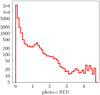 |
Fig. 4. Distribution of the standard deviation among the three photometric redshift estimates yielded for each object by EAZY, LEPHARE, and Z-PHOT. For most of the objects the standard deviation is close to zero, indicating good agreement between the three codes. The values are included in the released catalogue as an indicator of the quality of the median value adopted as the final redshift estimate. |
Figures 5 and 6 summarise the accuracy of the results, showing the values of the ASTRODEEP-GS43 best photo-z estimates for the objects in the spec-z sample used for the zero-point correction calibration. Our final estimates have NMAD = 0.015 and η = 3.01%; considering only the bright objects (I814 < 22.5), we obtain NMAD = 0.011 and η = 0.22%, which is comparable to the values obtained by Ilbert et al. (2013) for their UltraVISTA DR1 30 band catalogue on COSMOS (with the ‘zCOSMOS bright’ sample of ∼9400 spectroscopic redshifts at i+ < 22.5, they find NMAD = 0.008 and η = 0.6%). The first three panels of Fig. 5 as well as Fig. 6 show the comparison of the photometric and spectroscopic redshifts for each of the three independent runs and for the final median average, also reporting the NMAD and η statistics. The three runs yield comparable accuracy, with EAZY giving slightly better results on the full sample and LEPHARE giving slightly better results on the bright tail. It should be noted that the percentage of outliers for the bright tail is the same for all codes due to the fact that only one source is outside the range in all three of the runs.
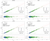 |
Fig. 5. Comparison of photometric and spectroscopic redshifts for the runs of (from left to right, top to bottom) the three codes, LEPHARE, EAZY, and Z-PHOT, plus (bottom right panel) the official CANDELS estimates from Dahlen et al. (2013). Green points are the full sample of 3931 spectroscopic sources described in Sect. 5.3.1, while the blue points are the bright tail with I814 < 22.5. In each case, the top sub-panel directly shows photo-z vs. spec-z, while the bottom sub-panel shows the corresponding Δz/(1 + zspec) distribution; the small inner sub-panel in the bottom right corner also show the same quantity as a histogram, along with the values of the median and standard deviations. See the text for more details. |
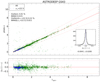 |
Fig. 6. Comparison of photometric and spectroscopic redshifts for the best estimate obtained as the median between the three single runs. Green points are the full sample of 3931 spectroscopic sources described in Sect. 5.3.1, while the blue points are the bright tail with I814 < 22.5. The top sub-panel directly shows photo-z vs. spec-z, while the bottom sub-panel shows the corresponding Δz/(1 + zspec) distribution; the small inner sub-panel in the bottom right corner also shows the same quantity as a histogram, along with the values of the median and standard deviations. |
5.4. Additional K- and IRAC-detected sources
For the additional Ks- and IRAC-detected sources, we only used ZPHOT to estimate the redshifts, with the same library of models described in Sect. 5.3; since no spectroscopic redshifts are available for calibration, we used the same zero-point corrections obtained for the H-band catalogue. Figure 7 displays the distribution of the evaluated redshifts for the three samples in the catalogue (the G13 list, the 173 new K detections, and the five IRAC detections).
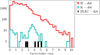 |
Fig. 7. Redshift distribution of the three samples in this work: the G13 CANDELS H-detected catalogue (red), the 173 K-detected sources (cyan), and the five additional IRAC-detected sources from W16 (black). |
5.5. Physical properties
We used Z-PHOT to evaluate the physical parameters of all the sources, keeping the redshift fixed to the best estimate obtained as described above and using the BC03 library, including nebular emission lines. We made two runs, one with standard exponentially declining SFHs (τ models) and one with delayed-τ models (see Sect. 5.3); in the final catalogue we list stellar masses and SFRs, with the corresponding 1σ uncertainties, for both of these runs.
To further verify the overall quality of the fit and check whether any band has problematic photometry, we used these last Z-PHOT runs to check, in each of the 43 bands, the fraction of objects whose best-fit flux strongly deviates (i.e. by more than 5σ) from the observed flux. The results are shown in Fig. 8. For the τ model run, on average only 2.1% (1.3%) of the sources are not well represented by the best fitting templates within these limits considering the wide (medium) bands, the two bands with the worst performance being ACS F606W and IRAC CH4; even in these two cases, however, the fraction of strongly deviating sources is, respectively, ∼4% and ∼3% of the total number of catalogue entries. The results for the delayed-τ run are similar.
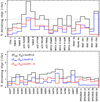 |
Fig. 8. Percentage of objects whose photo-z best-fit flux in the Z-PHOT run for the estimation of the physical parameters deviates by more than 5σ from the observed one in any given band. Shown is the result for the τ model run; the results for the delayed τ models are very similar. Upper and lower panels: wide and medium bands, respectively. The total fraction of deviating objects is given by the black histogram, while the blue and red histograms show objects whose best fit underestimates or overestimates, respectively, the observed flux. The dotted horizontal line is the median value for the considered set of passbands (for the totals, these are 2.1% for the wide bands and 1.3% for the medium bands). |
Finally, we assigned a quality flag to each source, for both runs, considering the (non-normalised) χ2 of the fitting processes. We visually inspected the fitted SEDs of a random sample of objects and statistically evaluated the distribution of χ2 values, finding that χ2 = 5 is a reasonable watershed between acceptable and non-satisfying unsatisfactory results. We also assigned separate flags to stars, identified as described in Sect. 5.2, and to AGNs, using the catalogue by Cappelluti et al. (2016) together with the VANDELS DR4 data (however, we are still releasing the photo-z and physical parameters estimates for AGNs). The flags are described in Table 3 (the fractions are from the delayed-τ fit, but they are almost identical for the τ run); with the chosen criteria, ∼6% of the objects are assigned a bad flag, indicating an unreliable fit.
Quality flags for physical parameters.
5.6. Comparison with CANDELS data
To conclude our analysis, we compared our best photometric redshift estimates with the official CANDELS results provided in the catalogue’s data release (Dahlen et al. 2013). The results in terms of the photo-z versus spec-z comparison for the CANDELS catalogue are shown in the fourth panel of Fig. 5. The new ASTRODEEP-GS43 redshift estimates reach a higher accuracy both in terms of the NMAD and of the outlier fraction.
In Fig. 9 we show the SED fitting of six sources with spectroscopic redshifts, which have improved the photometric redshift estimate with respect to the CANDELS fit. The combination of (i) the higher quality of the images, (ii) the new photometric software, (iii) the finer wavelength coverage (thanks to the addition of the medium bands), and (iv) the method adopted to evaluate the redshifts yields a high accuracy in the determination of the best-fit model of the source. This allows for an optimal tracing of the underlying spectral features, and therefore of a good photo-z estimate, which in the displayed cases is closer to the spectroscopic value than the CANDELS one. Statistically, these cases are more numerous than the opposite, leading to an overall improvement in the global accuracy of the photo-z estimate, as discussed above.
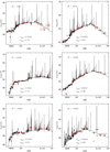 |
Fig. 9. Six examples of SED fitting of photometric sources exploiting the full 43 band dataset. Red squares are the CANDELS photometry from G13, black squares are the new photometric measurements, and the solid line is the best-fit model for the redshift estimate. In these cases, the improved photometric coverage leads to enhanced accuracy in the fit and, consequently, in the photo-z estimates (reported in the plots) with respect to the CANDELS estimates. Globally, this yields an overall improvement in the accuracy of the photometric redshifts, as discussed in Sect. 5.3.2. |
We also compared our statistics with those by Kodra (2019), who combined four independent redshift estimates on the original 17 band G13 catalogue using the minimum Frechet distance method; we take their mFDa4_weight estimate, which is the one they chose as ‘best’ in the absence of spectroscopic values. Also in this case, we find better overall results, their statistics being NMAD = 0.027 (0.023 for mI < 22.5) and η = 4.46% (0.22%). We verified that this result mainly depends on the improved photometric quality and wavelengths coverage since, taking the median of the EAZY, LEPHARE, and Z-PHOT runs used in Kodra’s analysis (i.e. the original CANDELS estimates), we find that the statistics are still worse than those we get for our new data.
Figure 10 shows the comparison between the new stellar masses (shown are the values obtained with the τ model runs) and the CANDELS ones from Santini et al. (2015, we used the 6a_tau_NEB estimate for consistency with the new models); we applied a conversion factor of 1.75 to compensate for the different IMF, which is Chabrier (2003) for CANDELS and Salpeter (1955) for ASTRODEEP-GS43. The agreement is good, except of course for the objects that have significantly different estimated redshifts in the two catalogues; for the galaxies with |zCANDELS − zGS43|< 0.1, the mean relative difference in mass is 26.3%, and the two estimates have distributions that are consistent within the error budget (for 67.7% of the galaxies, the CANDELS value is within the 1σ confidence interval of the new mass estimate).
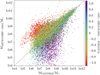 |
Fig. 10. Comparison of masses obtained with the Z-PHOT code in the four τ model runs for this work and in the official CANDELS catalogue. The IMF is Chabrier (a factor 1/1.75 has been applied to the new masses since the IMF in the new runs was assumed to be Salpeter); the SFH is from τ models. The colour code is proportional to the difference in photo-z. |
Finally, Fig. 11 shows a colour-mass diagram (H160−3.6 μm vs. stellar mass) of a sub-sample of the catalogue and of the corresponding CANDELS catalogue. In the left panels, colour and stellar mass are from the GS43 catalogue; in the right panels they are from CANDELS, respectively from G13 and Santini et al. (2015, we again used the 6a_tau_NEB estimate). In the upper panels we show the sources that are detected (S/N > 1) in IRAC CH1 in GS43 but which are upper limits in G13; the lower panels show the opposite case. Thanks to the combination of the new deeper mosaics and the new improved photometry with T-PHOT, in ASTRODEEP-GS43 we gain 6369 detections while losing just 878. We note that some sources that had been catalogued as red and massive in CANDELS, having CH1 detections at > 1σ, now appear to be upper limits (this is likely due to the fact that T-PHOT allowed for a better decontamination from neighbouring objects, lowering their flux).
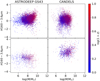 |
Fig. 11. Compared colour-mass diagrams (H160−3.6 μm vs. stellar mass) of the GS43 and CANDELS catalogues, colour-coded as a function of redshift. Left panels: stellar mass and colour are from the GS43 catalogue; right panels: they are from CANDELS, with photometry from G13 and masses from Santini et al. (2015); in both cases we considered the standard τ models that include emission lines. Upper panels: sources that in GS43 are detected (S/N > 1) in IRAC CH1 and are upper limits in G13; the lower panels show the opposite. |
6. Summary and conclusions
We have presented ASTRODEEP-GS43, a new photometric catalogue for the GOODS-South field, which includes 43 passbands (we are releasing total fluxes and corresponding 1σ uncertainties), photometric redshifts for sources without an available spectroscopic estimate, and physical properties (the stellar mass and SFR) of 35 108 objects: 34 930 are the H-detected objects from the original CANDELS G13 catalogue, 173 are additional sources detected in Ks, and five are additional sources detected in IRAC bands (these five are from the W16 study, including two that were not present in their original published list).
The new ASTRODEEP-GS43 redshift and physical parameter estimates proved to be consistent with previous releases. Thanks to: (i) the use of new, deeper images for HST ACS and Spitzer IRAC bands, (ii) the adoption of new techniques for photometric measurements (T-PHOT v2.0 with adaptive prioring, background subtraction, individual kernels, and astrometric registration), and (iii) the combination of different software tools for photometric redshift estimates (LEPHARE, EAZY, and Z-PHOT), comparisons with the official CANDELS data show an overall good agreement, with a noticeable improvement in the quality of the photometric redshift estimates, which reach NMAD = 0.015 and η = 3%; considering only the bright objects (I814 < 22.5), we obtain NMAD = 0.011 and η = 0.22%.
The catalogue is available for download from the ASTRODEEP website7 and from the CDS.
We applied this procedure directly for ZPHOT and EAZY, while for LEPHARE we took advantage of the dedicated option on the remote GAZPAR portal.
The NMAD is defined as 1.48 × median(|zphot − zspec|/(1 + zspec)).
Acknowledgments
Part of this study was funded using the EU FP7SPACE project ASTRODEEP (ref. no: 312725), supported by the European Commission. This work is partly based on tools and data products produced by GAZPAR operated by CeSAM-LAM and IAP. This research has made use of the SVO Filter Profile Service (http://svo2.cab.inta-csic.es/theory/fps/) supported from the Spanish MINECO through grant AYA2017-84089. The Cosmic Dawn Center is funded by the Danish National Research Foundation under grant no. 140. BMJ is supported in part by Independent Research Fund Denmark grant DFF – 7014-00017. The authors thank Tao Wang and Mengyuan Xiao for their contributions to the work.
References
- Arnouts, S., Cristiani, S., Moscardini, L., et al. 1999, MNRAS, 310, 540 [NASA ADS] [CrossRef] [Google Scholar]
- Ashby, M. L. N., Stanford, S. A., Brodwin, M., et al. 2013, ApJS, 209, 22 [NASA ADS] [CrossRef] [Google Scholar]
- Ashby, M. L. N., Willner, S. P., Fazio, G. G., et al. 2015, ApJS, 218, 33 [NASA ADS] [CrossRef] [Google Scholar]
- Bertin, E., & Arnouts, S. 1996, A&AS, 117, 393 [NASA ADS] [CrossRef] [EDP Sciences] [Google Scholar]
- Bertin, E., Mellier, Y., Radovich, M., et al. 2002, in Astronomical Data Analysis Software and Systems XI, eds. D. A. Bohlender, D. Durand, & T. H. Handley, ASP Conf. Ser., 281, 228 [NASA ADS] [Google Scholar]
- Brammer, G. B., van Dokkum, P. G., & Coppi, P. 2008, ApJ, 686, 1503 [NASA ADS] [CrossRef] [Google Scholar]
- Bruzual, G., & Charlot, S. 2003, MNRAS, 344, 1000 [NASA ADS] [CrossRef] [Google Scholar]
- Calzetti, D., Armus, L., Bohlin, R. C., et al. 2000, ApJ, 533, 682 [NASA ADS] [CrossRef] [Google Scholar]
- Cappelluti, N., Comastri, A., Fontana, A., et al. 2016, ApJ, 823, 95 [NASA ADS] [CrossRef] [Google Scholar]
- Cardamone, C. N., van Dokkum, P. G., Urry, C. M., et al. 2010, ApJS, 189, 270 [NASA ADS] [CrossRef] [Google Scholar]
- Castellano, M., Fontana, A., Paris, D., et al. 2010, A&A, 524, A28 [NASA ADS] [CrossRef] [EDP Sciences] [Google Scholar]
- Castellano, M., Sommariva, V., Fontana, A., et al. 2014, A&A, 566, A19 [NASA ADS] [CrossRef] [EDP Sciences] [Google Scholar]
- Castellano, M., Amorín, R., Merlin, E., et al. 2016, A&A, 590, A31 [NASA ADS] [CrossRef] [EDP Sciences] [Google Scholar]
- Chabrier, G. 2003, PASP, 115, 763 [Google Scholar]
- Daddi, E., Cimatti, A., Renzini, A., et al. 2004, ApJ, 617, 746 [Google Scholar]
- Dahlen, T., Mobasher, B., Faber, S. M., et al. 2013, ApJ, 775, 93 [Google Scholar]
- Di Criscienzo, M., Merlin, E., Castellano, M., et al. 2017, A&A, 607, A30 [NASA ADS] [CrossRef] [EDP Sciences] [Google Scholar]
- Elbaz, D., Dickinson, M., Hwang, H. S., et al. 2011, A&A, 533, A119 [NASA ADS] [CrossRef] [EDP Sciences] [Google Scholar]
- Fontana, A., D’Odorico, S., Poli, F., et al. 2000, AJ, 120, 2206 [NASA ADS] [CrossRef] [Google Scholar]
- Fontana, A., Dunlop, J. S., Paris, D., et al. 2014, A&A, 570, A11 [NASA ADS] [CrossRef] [EDP Sciences] [Google Scholar]
- Franco, M., Elbaz, D., Béthermin, M., et al. 2018, A&A, 620, A152 [NASA ADS] [CrossRef] [EDP Sciences] [Google Scholar]
- Galametz, A., Grazian, A., Fontana, A., et al. 2013, ApJS, 206, 10 [NASA ADS] [CrossRef] [Google Scholar]
- Garilli, B., McLure, R., Pentericci, L., et al. 2021, A&A, 647, A150 [NASA ADS] [CrossRef] [EDP Sciences] [Google Scholar]
- Grazian, A., Salimbeni, S., Pentericci, L., et al. 2007, A&A, 465, 393 [NASA ADS] [CrossRef] [EDP Sciences] [Google Scholar]
- Grazian, A., Fontana, A., Santini, P., et al. 2015, A&A, 575, A96 [NASA ADS] [CrossRef] [EDP Sciences] [Google Scholar]
- Grogin, N. A., Kocevski, D. D., Faber, S. M., et al. 2011, ApJS, 197, 35 [NASA ADS] [CrossRef] [Google Scholar]
- Guo, Y., Ferguson, H. C., Giavalisco, M., et al. 2013, ApJS, 207, 24 [NASA ADS] [CrossRef] [Google Scholar]
- Ilbert, O., Arnouts, S., McCracken, H. J., et al. 2006, A&A, 457, 841 [NASA ADS] [CrossRef] [EDP Sciences] [Google Scholar]
- Ilbert, O., Capak, P., Salvato, M., et al. 2009, ApJ, 690, 1236 [NASA ADS] [CrossRef] [Google Scholar]
- Ilbert, O., McCracken, H. J., Le Fèvre, O., et al. 2013, A&A, 556, A55 [NASA ADS] [CrossRef] [EDP Sciences] [Google Scholar]
- Illingworth, G., Magee, D., Bouwens, R., et al. 2016, ArXiv e-prints [arXiv:1606.00841] [Google Scholar]
- Kodra, D. 2019, PhD Thesis, University of Pittsburgh, USA [Google Scholar]
- Koekemoer, A. M., Faber, S. M., Ferguson, H. C., et al. 2011, ApJS, 197, 36 [NASA ADS] [CrossRef] [Google Scholar]
- Koekemoer, A. M., Avila, R. J., Hammer, D., et al. 2014, Am. Astron. Soc. Meet. Abstr., 223, 254.02 [Google Scholar]
- Labbé, I., Oesch, P. A., Illingworth, G. D., et al. 2015, ApJS, 221, 23 [NASA ADS] [CrossRef] [Google Scholar]
- Laidler, V. G., Papovich, C., Grogin, N. A., et al. 2007, PASP, 119, 1325 [Google Scholar]
- Lotz, J., Mountain, M., Grogin, N. A., et al. 2014, Am. Astron. Soc. Meet. Abstr., 223, 254.01 [NASA ADS] [Google Scholar]
- Luo, B., Brandt, W. N., Xue, Y. Q., et al. 2017, ApJS, 228, 2 [Google Scholar]
- McLure, R. J., Pentericci, L., Cimatti, A., et al. 2018, MNRAS, 479, 25 [NASA ADS] [Google Scholar]
- Merlin, E., Fontana, A., Ferguson, H. C., et al. 2015, A&A, 582, A15 [NASA ADS] [CrossRef] [EDP Sciences] [Google Scholar]
- Merlin, E., Bourne, N., Castellano, M., et al. 2016a, A&A, 595, A97 [NASA ADS] [CrossRef] [EDP Sciences] [Google Scholar]
- Merlin, E., Amorín, R., Castellano, M., et al. 2016b, A&A, 590, A30 [NASA ADS] [CrossRef] [EDP Sciences] [Google Scholar]
- Merlin, E., Fontana, A., Castellano, M., et al. 2018, MNRAS, 473, 2098 [NASA ADS] [CrossRef] [Google Scholar]
- Merlin, E., Fortuni, F., Torelli, M., et al. 2019, MNRAS, 490, 3309 [NASA ADS] [CrossRef] [Google Scholar]
- Nonino, M., Dickinson, M., Rosati, P., et al. 2009, ApJS, 183, 244 [NASA ADS] [CrossRef] [Google Scholar]
- Oke, J. B., & Gunn, J. E. 1983, ApJ, 266, 713 [NASA ADS] [CrossRef] [Google Scholar]
- Pentericci, L., McLure, R. J., Garilli, B., et al. 2018, A&A, 616, A174 [NASA ADS] [CrossRef] [EDP Sciences] [Google Scholar]
- Polletta, M., Tajer, M., Maraschi, L., et al. 2007, ApJ, 663, 81 [NASA ADS] [CrossRef] [Google Scholar]
- Rodrigo, C., Solano, E., & Bayo, A. 2012, SVO Filter Profile Service Version 1.0, IVOA Working Draft 15 October 2012 [Google Scholar]
- Salpeter, E. E. 1955, ApJ, 121, 161 [Google Scholar]
- Salpeter, E. E. 1959, ApJ, 129, 608 [NASA ADS] [CrossRef] [Google Scholar]
- Santini, P., Ferguson, H. C., Fontana, A., et al. 2015, ApJ, 801, 97 [NASA ADS] [CrossRef] [Google Scholar]
- Schaerer, D., & de Barros, S. 2009, A&A, 502, 423 [NASA ADS] [CrossRef] [EDP Sciences] [Google Scholar]
- Shipley, H. V., Lange-Vagle, D., Marchesini, D., et al. 2018, ApJS, 235, 14 [NASA ADS] [CrossRef] [Google Scholar]
- Skelton, R. E., Whitaker, K. E., Momcheva, I. G., et al. 2014, ApJS, 214, 24 [Google Scholar]
- Stefanon, M., Yan, H., Mobasher, B., et al. 2017, ApJS, 229, 32 [NASA ADS] [CrossRef] [Google Scholar]
- Straatman, C. M. S., Spitler, L. R., Quadri, R. F., et al. 2016, ApJ, 830, 51 [NASA ADS] [CrossRef] [Google Scholar]
- Wang, T., Elbaz, D., Schreiber, C., et al. 2016, ApJ, 816, 84 [Google Scholar]
- Whitaker, K. E., Ashas, M., Illingworth, G., et al. 2019, ApJS, 244, 16 [CrossRef] [Google Scholar]
Appendix A: Photometric comparisons with other catalogues
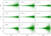 |
Fig. A.1. Comparison of measured magnitudes between this work and the original CANDELS G13 catalogue for nine reference bands. |
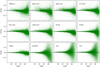 |
Fig. A.2. Comparison of measured magnitudes between this work and the 3D-HST catalogue for 12 reference bands. |
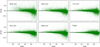 |
Fig. A.3. Comparison of measured magnitudes between this work and the HLF catalogue for six reference bands (ACS). |
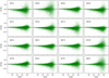 |
Fig. A.4. Comparison of measured magnitudes between this work and the MUSYC catalogue for 16 reference medium bands. |
Appendix B: Description of the ASTRODEEP-GS43 catalogue
The sources in the catalogue are ordered by their IDs. The first 34930 are the H-detected ones from G13; the subsequent ones are the new Ks- and IRAC-detected sources discussed in Sect. 3.1.
We are releasing two separate files in ASCII format. The first, named ASTRODEEP-GS43_phot.cat, includes IDs, coordinates (RA and Dec), and the 43 band photometry (not cleaned for the photo-z estimation described in Sect. 5.3.1); the passbands are listed in order of increasing wavelength, and we provide total fluxes and corresponding uncertainties in microjanskys. The second, ASTRODEEP-GS43_phys.cat, includes (i) the best redshift estimation, that is, the spectroscopic z when available (including the original reference), or the median of the three photometric redshifts obtained with LEPHARE, EAZY, and Z-PHOT otherwise, along with the three estimates and their standard deviations, and (ii) two physical parameters obtained from the best fitting template SED, namely stellar mass and SFR, with 1σ uncertainties (given as lower and upper values of the 68% confidence interval), plus the quality flag described in Sect. 5.5, for two SFH models, namely exponentially declining (tau) and delayed exponentially declining (deltau; see Sect. 5.3 for details).
All Tables
All Figures
|
Fig. 1. Complete passband set for the ASTRODEEP-GS43 catalogue. Upper panel: filters of the SUPRIMECAM and FOURSTAR bands, while the lower panel: wide bands from HST, Spitzer, and ground-based facilities; the curves are normalised to arbitrary units to make them peak at unitary transmission. |
| In the text | |
|
Fig. 2. Examples of new K-detected sources. Left to right: WFC3 H160, HAWK-I Ks, and T-PHOT residual on Ks. Upper panels (cyan circles): examples of sources detected with Method 1 (SEXTRACTOR in dual mode and cross-matching with G13). Lower panels (blue circles): examples of sources detected with Method 2 (K-band residual image with T-PHOT). See the text for details. |
| In the text | |
|
Fig. 3. From left to right: portion of the IRAC 3.6 μm mosaic by R. McLure; residuals after T-PHOT standard fitting using a single convolution kernel; residuals after fitting using a different individual kernel for each source, tailored on the basis of the positional angles of the pointings used to build the mosaic and with the T-PHOT global background subtraction option switched on; residuals for the final run, where the T-PHOT individual kernel registration option is also switched on (in the last two panels, blue boxes highlight regions where the improvement using this technique is evident). See the text for more details on the methods. |
| In the text | |
|
Fig. 4. Distribution of the standard deviation among the three photometric redshift estimates yielded for each object by EAZY, LEPHARE, and Z-PHOT. For most of the objects the standard deviation is close to zero, indicating good agreement between the three codes. The values are included in the released catalogue as an indicator of the quality of the median value adopted as the final redshift estimate. |
| In the text | |
|
Fig. 5. Comparison of photometric and spectroscopic redshifts for the runs of (from left to right, top to bottom) the three codes, LEPHARE, EAZY, and Z-PHOT, plus (bottom right panel) the official CANDELS estimates from Dahlen et al. (2013). Green points are the full sample of 3931 spectroscopic sources described in Sect. 5.3.1, while the blue points are the bright tail with I814 < 22.5. In each case, the top sub-panel directly shows photo-z vs. spec-z, while the bottom sub-panel shows the corresponding Δz/(1 + zspec) distribution; the small inner sub-panel in the bottom right corner also show the same quantity as a histogram, along with the values of the median and standard deviations. See the text for more details. |
| In the text | |
|
Fig. 6. Comparison of photometric and spectroscopic redshifts for the best estimate obtained as the median between the three single runs. Green points are the full sample of 3931 spectroscopic sources described in Sect. 5.3.1, while the blue points are the bright tail with I814 < 22.5. The top sub-panel directly shows photo-z vs. spec-z, while the bottom sub-panel shows the corresponding Δz/(1 + zspec) distribution; the small inner sub-panel in the bottom right corner also shows the same quantity as a histogram, along with the values of the median and standard deviations. |
| In the text | |
|
Fig. 7. Redshift distribution of the three samples in this work: the G13 CANDELS H-detected catalogue (red), the 173 K-detected sources (cyan), and the five additional IRAC-detected sources from W16 (black). |
| In the text | |
|
Fig. 8. Percentage of objects whose photo-z best-fit flux in the Z-PHOT run for the estimation of the physical parameters deviates by more than 5σ from the observed one in any given band. Shown is the result for the τ model run; the results for the delayed τ models are very similar. Upper and lower panels: wide and medium bands, respectively. The total fraction of deviating objects is given by the black histogram, while the blue and red histograms show objects whose best fit underestimates or overestimates, respectively, the observed flux. The dotted horizontal line is the median value for the considered set of passbands (for the totals, these are 2.1% for the wide bands and 1.3% for the medium bands). |
| In the text | |
|
Fig. 9. Six examples of SED fitting of photometric sources exploiting the full 43 band dataset. Red squares are the CANDELS photometry from G13, black squares are the new photometric measurements, and the solid line is the best-fit model for the redshift estimate. In these cases, the improved photometric coverage leads to enhanced accuracy in the fit and, consequently, in the photo-z estimates (reported in the plots) with respect to the CANDELS estimates. Globally, this yields an overall improvement in the accuracy of the photometric redshifts, as discussed in Sect. 5.3.2. |
| In the text | |
|
Fig. 10. Comparison of masses obtained with the Z-PHOT code in the four τ model runs for this work and in the official CANDELS catalogue. The IMF is Chabrier (a factor 1/1.75 has been applied to the new masses since the IMF in the new runs was assumed to be Salpeter); the SFH is from τ models. The colour code is proportional to the difference in photo-z. |
| In the text | |
|
Fig. 11. Compared colour-mass diagrams (H160−3.6 μm vs. stellar mass) of the GS43 and CANDELS catalogues, colour-coded as a function of redshift. Left panels: stellar mass and colour are from the GS43 catalogue; right panels: they are from CANDELS, with photometry from G13 and masses from Santini et al. (2015); in both cases we considered the standard τ models that include emission lines. Upper panels: sources that in GS43 are detected (S/N > 1) in IRAC CH1 and are upper limits in G13; the lower panels show the opposite. |
| In the text | |
|
Fig. A.1. Comparison of measured magnitudes between this work and the original CANDELS G13 catalogue for nine reference bands. |
| In the text | |
|
Fig. A.2. Comparison of measured magnitudes between this work and the 3D-HST catalogue for 12 reference bands. |
| In the text | |
|
Fig. A.3. Comparison of measured magnitudes between this work and the HLF catalogue for six reference bands (ACS). |
| In the text | |
|
Fig. A.4. Comparison of measured magnitudes between this work and the MUSYC catalogue for 16 reference medium bands. |
| In the text | |
Current usage metrics show cumulative count of Article Views (full-text article views including HTML views, PDF and ePub downloads, according to the available data) and Abstracts Views on Vision4Press platform.
Data correspond to usage on the plateform after 2015. The current usage metrics is available 48-96 hours after online publication and is updated daily on week days.
Initial download of the metrics may take a while.