| Issue |
A&A
Volume 649, May 2021
|
|
|---|---|---|
| Article Number | A161 | |
| Number of page(s) | 12 | |
| Section | Extragalactic astronomy | |
| DOI | https://doi.org/10.1051/0004-6361/202040186 | |
| Published online | 01 June 2021 | |
Assembly history of massive galaxies
A pilot project with VEGAS deep imaging and M3G integral field spectroscopy
1
INAF-Astronomical Observatory of Capodimonte, Salita Moiariello 16, 80131 Naples, Italy
e-mail: This email address is being protected from spambots. You need JavaScript enabled to view it.
2
Leibniz-Institut für Astrophysik Potsdam (AIP), An der Sternwarte 16, 14482 Potsdam, Germany
3
European Southern Observatory, Karl-Schwarzschild-Str. 2, 85748 Garching, Germany
Received:
21
December
2020
Accepted:
12
March
2021
Abstract
In this paper we present the new deep images from the VEGAS survey of three massive (M* ≃ 1012 M⊙) galaxies from the MUSE Most Massive Galaxies (M3G) project, with distances in the range 151 ≤ D ≤ 183 Mpc: PGC007748, PGC015524, and PGC049940. The long integration time and the wide field of view of the OmegaCam at the VST allowed us to map the light and color distributions down to μg ≃ 30 mag arcsec−2 and out to ∼2Re. The deep data are crucial for estimating the contribution of the different galaxy components, in particular the accreted fraction in the stellar halo. The available integral field observations with MUSE cover a limited portion of each galaxy (out to ∼1Re), but from the imaging analysis, we find that they map the kinematics and stellar population beyond the first transition radius, where the contribution of the accreted component starts to dominate. The main goal of this work is to correlate the scales of the different components derived from the image analysis with the kinematics and stellar population profiles from the MUSE data. The results were used to address the assembly history of the three galaxies with the help of theoretical predictions. Our results suggest that PGC049940 has the lowest accreted mass fraction of 77%. The higher accreted mass fraction estimated for PGC007748 and PGC015524 (86% and 89%, respectively) combined with the flat λR profiles suggest that a great majority of the mass has been acquired through major mergers, which have also shaped the shallower metallicity profiles that are observed at larger radii.
Key words: techniques: image processing / galaxies: elliptical and lenticular, cD / galaxies: fundamental parameters / galaxies: formation / galaxies: clusters: general
© ESO 2021
1. Introduction
From the observational and theoretical side, it is broadly accepted that the stellar mass of the present-day massive (M* ≃ 3 × 10¹¹ M⊙) and passive early-type galaxies (ETGs) results from the gradual accretion of satellites that form the extended stellar halo around a compact spheroid (e.g., Kormendy et al. 2009; van Dokkum & Conroy 2010; Huang et al. 2018; Spavone et al. 2017). The accreted stellar content in ETGs that comes from the mass assembly in the stellar halo formed the ex situ component. This component mixed with the in situ component at small radii. The properties of in situ stars in the light distribution, kinematics, and stellar populations are different from those in the ex situ region.
Simulations show that in the surface-brightness radial profiles of galaxies, we may expect a “transition radius” (Rtr), corresponding to variations in the ratio between the accreted ex situ and the in situ components (Cooper et al. 2010; Deason et al. 2013; Amorisco 2017). The simulated profiles are described by a first component identifying the stars that formed in situ, and by a second and third component representing the relaxed and unrelaxed accreted stars, respectively. The radius marking the transition between each of these components is defined as the transition radius. Massive galaxies with a high accreted mass fraction are assumed to have a small first Rtr (Cooper et al. 2010, 2013). The outer stellar envelope should appear as a shallower exponential profile at larger radii after a second transition radius in the surface brightness distribution. On the observational side, the study of the surface brightness profiles of ETGs out to the faintest levels therefore turned out to be one of the main tools for quantifying the contribution of the accreted mass. This method becomes particularly efficient when the outer stellar envelope starts to be dominant beyond the second transition radius (Seigar et al. 2007; Iodice et al. 2016, 2017a; Spavone et al. 2017, 2018, 2020).
To this aim, recent deep-imaging surveys of nearby groups and clusters of galaxies have provided extensive analyses of the light and color distribution of the brightest and massive members out to the regions of the stellar halos where the imprints of the mass assembly can be recognized (e.g., Duc et al. 2015; Capaccioli et al. 2015; Trujillo & Fliri 2016; Mihos et al. 2017; Spavone et al. 2018; Iodice et al. 2019, 2020b).
The VST Early-type GAlaxies Survey (VEGAS1, P.I. E. Iodice, Capaccioli et al. 2015) has recently occupied a pivotal role in exploring the low-surface brightness universe and studying galaxy properties as function of the environment. VEGAS data allowed us to (i) study the galaxy outskirts, detect the intracluster light (ICL) and low surface brightness (LSB) features in the intracluster and group space (Spavone et al. 2018; Cattapan et al. 2019; Iodice et al. 2020b; ii) trace the mass assembly in galaxies by estimating the accreted mass fraction in the stellar halos and providing results that can be directly compared with predictions of galaxy formation models (Spavone et al. 2017, 2020); (iii) provide the spatial distribution of candidate globular clusters (GCs) in the galaxy outskirts and in the intracluster space (Cantiello et al. 2018); and (iv) detect ultra-diffuse galaxies (UDGs, Forbes et al. 2019, 2020; Iodice et al. 2020a).
The stellar kinematics and population properties from the integrated light (e.g., Coccato et al. 2010, 2011; Ma et al. 2014; Barbosa et al. 2018; Veale et al. 2018; Greene et al. 2019) and kinematics of discrete tracers such as GCs and planetary nebulae (PNe) (e.g., Coccato et al. 2013; Longobardi et al. 2013; Spiniello et al. 2018; Hartke et al. 2018; Pulsoni et al. 2020, 2021) have also been used to trace the mass assembly in the outer regions of galaxies. In this field, key results are on the stellar population gradients out to the region of the stellar halos. They indicate a different star formation history in the central in situ component from that in the galaxy outskirts (e.g., Greene et al. 2015; McDermid et al. 2015; Barone et al. 2018; Ferreras et al. 2019). Moreover, PNe and GCs have also been used as kinematic tracers. In some cases, they show different kinematics than the central regions (Coccato et al. 2009; Foster et al. 2013; Arnold et al. 2014).
As the integral field units become larger, it is possible to map a significant area of galaxies. A survey that mapped massive galaxies out to two effective radii is the MUSE Most Massive Galaxies (M3G; PI: E. Emsellem) survey. The main aim of this survey is to map the most massive galaxies in the densest galaxy environments at z ∼ 0.045 with the MUSE spectrograph at the Very Large Telescope (VLT; Bacon et al. 2010). The M3G is a survey of 25 massive galaxies in dense environments, whose stellar velocity maps have been published in Krajnović et al. (2018). The survey has shown that a large fraction of the galaxies in the sample have a prolate-like rotation.
All these findings from photometry and spectroscopy are consistent with the theoretical prediction for the formation and evolution of ETGs (Cooper et al. 2013; Pillepich et al. 2018; Schulze et al. 2020; Cook et al. 2016). In particular, the surface brightness and metallicity profiles appear to be shallower in the outskirts when repeated mergers occur (Cook et al. 2016), that is, when the accreted fraction of metal-rich stars increases.
Moreover, using Magneticum Pathfinder simulations, Schulze et al. (2020) reported a correlation between the shape of λR and the galaxy accretion history. In addition, they also found that the radius marking the kinematic transition between different galaxy components provides a good estimate of the transition radius between the in situ and accreted component in the photometric profiles.
The excellent quality of photometric and spectroscopic data from VEGAS and M3G provides the unique opportunity of linking the deep (> 29 mag arcsec−2) optical photometry extending to several half-light radii (Re) and the MUSE spectroscopic data (stellar kinematics and stellar populations) within the central 2Re.
The main goal of this work is to correlate the scales of different galaxy components set from the deep photometry with the kinematics and stellar population properties derived from the integral field spectroscopy. While MUSE observations of massive galaxies in the nearby universe (within the M3G survey) provide spectroscopically derived constraints on their formation history (through stellar and gas kinematics and stellar populations), they are limited to the central one to two effective radii. Taking advantage of the extraordinary depth and extent of OmegaCam images from the VEGAS survey, we investigate the links between the central galaxy (spectroscopic) properties and the large-scale (photometric) structures for three brightest cluster galaxies (BCGs) in M3G. The VEGAS surface brightness and color profiles will serve as a key structural parameterization of the main galaxy components, including the relaxed and not relaxed stellar components, and an estimate of the accreted stellar mass. The MUSE data are then used to reveal potential signatures of transitions between the structural components in stellar kinematics, and angular momentum and age and metallicity distributions. The results, supported by detailed theoretical predictions, will help constrain the accretion histories of these targets.
This work is organized as follows. In Sect. 2 we describe the data (both photometric and spectroscopic) and briefly introduce the reduction steps. In Sect. 3 we present the data analysis, and in Sect. 4 we show the adopted procedure for fitting the surface brightness profiles. In Sect. 5 we compare the observables derived from the surface photometry with the stellar population properties derived from MUSE data. In Sect. 6 we finally compare observational results with the theoretical predictions and draw our conclusions.
2. Observations and data reduction
2.1. Deep photometry
The photometric data we present are part of the VEGAS survey (Capaccioli et al. 2015). VEGAS is a multiband u, g, r, and i imaging survey carried out with the European Southern Observatory (ESO) Very Large Telescope Survey Telescope (VST). The VST is a 2.6 m wide-field optical telescope (Schipani et al. 2012) equipped with OmegaCAM, a 1° ×1° camera with a resolution of 0.21 arcsec pixel−1. The data we present in this work were acquired in the g and r bands in visitor mode (run IDs: 100.B-0168(A), 101.A-0166(A), 102.A-0669(A)) during dark time in photometric conditions, with an average seeing with a full width at half maximum (FWHM) of ∼1 arcsec in the g band and FWHM ∼ 0.7 arcsec in the r band. The total exposure time was 2.5 hours for each target and in each band.
All the imaging data were processed using the dedicated AstroWISE pipeline developed to reduce OmegaCam observations (McFarland et al. 2013; Venhola et al. 2018). The various steps of the AstroWise data reduction were extensively described in Venhola et al. (2017, 2018).
Because the angular extent of the galaxies is much smaller than the VST field, observations for these objects were performed using the standard diagonal dithering strategy. As described in Capaccioli et al. (2015) and Spavone et al. (2017), the background subtraction for the targets observed with this strategy is performed by fitting a surface, typically a 2D polynomial, to the pixel values of the mosaic that are unaffected by celestial sources or defects.
2.2. 2D spectroscopy
The spectroscopic data were taken from the M3G Survey, which mapped 25 galaxies found in dense environments. The sample and the data reduction were presented in Krajnović et al. (2018), and here we briefly outline the most relevant points. The M3G sample is built of galaxies brighter than −25.7 mag in the 2MASS Ks band, divided into two subsamples comprising 11 galaxies in the three richest (Abell et al. 1989) clusters of the Shapley supercluster and 14 BCGs selected from clusters that are richer than the Virgo cluster (three of them are also in the Shapley supercluster subsample). This paper analyses the three BCGs found both in VEGAS and M3G samples.
The data reduction was performed using the MUSE data reduction pipeline (Weilbacher et al. 2020), following the standard steps: producing the master bias and flat-field calibration files, the trace tables, wavelength calibration files, and line-spread function (LSF) for each slice. When available, we also used twilight flats. Instrument geometry and astrometry files were provided by the GTO team for each observing run. We used separate sky fields to construct the sky spectra, associated with the closest-in-time on-target exposure. The response function was obtained from the observation of a standard star (for each night), but there were no observations of telluric standards. In addition to the reduction steps explained by Krajnović et al. (2018), for this paper we also removed the telluric lines using the MOLECFIT software (Smette et al. 2015), which computes a theoretical absorption model based on a radiative transfer code and an atmospheric molecular line database. The main contribution to the telluric absorptions comes from the oxygen either in molecular form (γ and B bands) or as ozone (Choppuis land), and water (see Fig. 1 in Smette et al. 2015). MOLECFIT was applied to the full wavelength region of the MUSE data cubes. The final data cubes were obtained by merging all individual exposures.
3. Data analysis
3.1. Imaging
We used sky-subtracted and stacked images of each galaxy in the g and r bands to perform the photometric analysis. We first estimated any residual fluctuations in the sky-subtracted images. From this we obtained an estimate of the accuracy of our sky-subtraction. The procedure is the same as adopted in previous VEGAS papers (Capaccioli et al. 2015; Iodice et al. 2016; Spavone et al. 2017, 2018). In short, we extracted the azimuthally averaged intensity profile (using the IRAF task ELLIPSE, Jedrzejewski 1987) out to the edges of the frame by fixing both the position angle (PA) and the ellipticity (ϵ) of the galaxy from the sky-subtracted images of each galaxy, after masking all the bright sources (galaxies and stars) and background objects. From this profile, we estimated a residual background of ∼0.04 ± 0.02 counts in g and ∼0.10 ± 0.06 in r by extrapolating the outer trend. Based on this procedure, we also estimated the outermost radius where counts are consistent with the average background level. This limiting radius sets the surface brightness limit of the VST light profiles. The limiting radii (Rlim) are ∼3 arcmin (∼160 kpc, Rlim/Re ∼ 7) for PGC007748, ∼10 arcmin (∼438 kpc, Rlim/Re ∼ 12) for PGC015524, and ∼12 arcmin (∼598 kpc, Rlim/Re ∼ 19) for PGC049948 in the g and r bands.
To account for the broadening effect of the seeing on the light distribution of galaxies, we used the point spread function (PSF) derived in Capaccioli et al. (2015) based on VST images, and deconvolved each galaxy in our sample for the VST PSF using the Richardson-Lucy (hereafter RL) algorithm (Lucy 1974; Richardson 1972). The robustness and the reliability of this deconvolution technique are shown in Spavone et al. (2020).
Before we analyzed the light distribution, 2D models of the bright stars close in projection to the galaxy under study were derived and subtracted from the image as required.
The isophotal analysis was performed with the IRAF2 task ELLIPSE, which provides the geometrical parameters and the light distribution azimuthally averaged within isophotal annuli of a specified thickness. The isophote fit was performed for each galaxy by masking all the bright sources in the field (stars and background galaxies). In this second ELLIPSE run, ϵ and PA were left free. From this analysis we derived ϵ and PA radial profiles, the azimuthally averaged surface brightness profiles in each band and the azimuthally averaged (g − r) color profiles. The results are shown in Figs. 1–3 for PGC007748, PGC015524, and PGC049940, respectively.
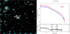 |
Fig. 1. Left panel: VST color-composite gr image of the 20.7 arcmin × 19.4 arcmin field around PGC 7748. Top right panel: azimuthally averaged surface brightness profiles in the g (blue) and r (red) bands. Bottom right panel: azimuthally averaged (g − r) color profile. The vertical dotted and dashed lines mark the position of the first and second transition radii, respectively, and the gray shaded areas are the transition regions (see Sect. 5). |
The growth curves obtained by isophote fitting were integrated and extrapolated to derive total magnitudes mT, effective radii Re, and corresponding effective magnitudes μe in each band (see Table1).
Distances and photometric parameters for the sample galaxies.
3.2. Spectroscopy
For the comparison with the imaging, we are primarily interested in two sets of spectroscopic data products: stellar kinematics and properties of stellar populations. In particular, we wish to characterize the radial profiles of the stellar velocity dispersion, stellar angular momentum, and stellar ages and metallicities.
The stellar kinematics was extracted in two steps. Based on the signal-to-noise ratio (S/N) of individual spectra, MUSE data cubes were binned using the Voronoi method (Cappellari & Copin 2003)3 to a target S/N of 50. This was followed by extraction of kinematics based assuming a Gaussian line-of-sight velocity distribution using the pPXF software (Cappellari & Emsellem 2004; Cappellari 2017)4. We masked the regions of possible emission lines and residual sky lines and fit the wavelength region blueward of 7000 Å by applying a 12th-order additive polynomial, which is appropriate for the long wavelength region used, as suggested by the analysis in Appendix A.4 of van de Sande et al. (2017). The wavelength limit is based on tests that showed that the extraction of kinematics in the blue part of MUSE spectra is fully consistent with the kinematics of the SAURON survey (Emsellem et al. 2004), while including the full MUSE spectrum can lead to inconsistencies (Krajnović et al. 2015). We masked all emission lines in this spectral range (i.e., Hβ [OIII]λ4959, 5007, [NI]λ5197, 5200, [OI]λ6300, 6364, [NII]λ6548, 6583, Hα, and [SII]λ6716, 6731) as well as any residual skylines (e.g., at 5557 Å and around 6300 Å). An example of a pPXF fit to M3G spectra together with the fitting region and masked wavelengths is provided in Krajnović et al. (2018). As templates we used the MILES library of stellar spectra (Sánchez-Blázquez et al. 2006; Falcón-Barroso et al. 2011), which were convolved to match the varying MUSE spectral resolution (Guérou et al. 2017) in the fitted spectral regions.
The stellar population parameters were similarly extracted using the pPXF, but this time using the E-MILES single stellar population (SSP) models (Vazdekis et al. 2016). We used SSP models based on the Padova isochrones (Girardi et al. 2000) and Kroupa (2001) initial mass function, with parameters distributed in a grid of log(age) between 0.1 and 14.1 Gyr and metallicities [Z/H] between −1.71 and 0.22. The pPXF fit assigns a weight to each of the SSP spectra, and the final age and metallicities were calculated for each bin as the mass- (or luminosity-) weighted averages of the SSP parameters (age and metallicity) using the weights assigned by the pPXF fit. To extract the stellar populations parameters, we applied only multiplicative polynomials of the 12th order, masked the emission lines as outlined above, and used the same fitting region (4850–7000 Å). Errors on the kinematic and line-strength parameters were obtained through 500 Monte Carlo simulations, where the original spectrum was perturbed by a random value drawn from the standard deviation of the residuals of the pPXF fits. We derived the mass- and luminosity-weighted metallicities and ages, but we present here only the luminosity-weighted parameters for consistency with other (luminosity-weighted) parameters that we used (SB, λR, and σ). Nevertheless, we verified that the results do not change if we had used mass-weighted metallicities and ages.
The outlined steps produced maps of the mean velocity and the velocity dispersion and also of the stellar ages and metallicities. We show these maps in Fig. 4. As we wish to compare the velocity dispersion, ages, and metallicities with the photometric radial profiles, we still needed to extract 1D information from MUSE maps. We did this using kinemetry (Krajnović et al. 2006), a method for analyzing kinematic maps based on the ideas of isophotometric ellipse fitting (as in, e.g., Jedrzejewski 1987). We used the ellipse parameters (radius, flattening, and the position angle) of the isophotal analysis (see Sect. 3.1) to extract the radial profiles of the velocity dispersion, age and metallicities with kinemetry by averaging the same areas of our galaxies as during the photometric analysis. In this way, the radial profiles of photometric and spectroscopic properties can be directly compared. In addition, we derived the radial profiles of specific stellar angular momentum,
 (1)
(1)
(Emsellem et al. 2007), calculated as a cumulative function within an increasing aperture. We used elliptical apertures, again based on the photometric analysis (same ellipses), allowing a direct comparison with the stellar population properties, kinematics, and the color properties derived from VEGAS. Errors on the kinemetric radial profiles were obtained by error propagation. The apparently small errors are understandable given the large number of individual bins we used to estimate parameters at each radius. The formal errors on the λR profiles were estimated by Monte Carlo variation of the velocity and the velocity dispersion, based on the derived uncertainties on these quantities.
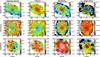 |
Fig. 4. Velocity, σ, metallicity, and age MUSE maps for the studied galaxies. The dashed black contours are isophotes. They are plotted in steps of half a magnitude. |
4. Fit of the surface brightness profiles
In recent years, a considerable number of observational works that took advantage of the deep photometry obtained with the new-generation telescopes, have demonstrated that the light profiles of many of the most massive ETGs are only poorly fit by a single Sérsic law and additional components are needed (Seigar et al. 2007; Donzelli et al. 2011; Arnaboldi et al. 2012; Iodice et al. 2016, 2020b; Spavone et al. 2017, 2018, 2020; Cattapan et al. 2019).
Spavone et al. (2017) followed the predictions of numerical simulations (Cooper et al. 2013, 2015) and described the surface brightness profiles of a sample of massive ETGs with a three-component model: a Sérsic component for the innermost galaxies’ regions, a second Sérsic component for the central regions, and an exponential component (Sérsic with n = 1) for the outskirts. In the simulated profiles, the first component identifies the stars formed in situ, and the second and third components represent the relaxed and unrelaxed accreted stars, respectively. Because our fitting procedure is simulations driven, it allows us to estimate the scales at which each stellar component starts to dominate the galaxy light profiles.
Following the procedure developed in Spavone et al. (2017), we modeled the light profiles of PGC007748, PGC015524, and PGC049940 with three-component fits in order to derive indications on the balance between the different components. Because these fits may be substantially degenerate between parameters, we adopted the typical value of the Sérsic index for the first component (n = 2 ± 0.5) on the basis of the results of theoretical simulations by Cooper et al. (2013) for massive galaxies (1010 ≤ M* ≤ 1013 M⊙) to mitigate this degeneracy. The results of the fits are shown in Fig. 5, and the best-fitting structural parameters are reported in Table 2.
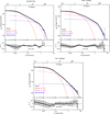 |
Fig. 5. VST g-band profile of PGC007748 (top left), PGC015524 (top right), and PGC049940 (bottom) in linear scale, fit with a three-component model motivated by the predictions of theoretical simulations (see Spavone et al. (2017)). The bottom panels in each plot show the Δ rms scatter, obtained from the difference between the observed profiles (O) and the sum of the components from each fit (C). The dashed lines in all the panels indicate the galaxy cores. |
Best-fitting structural parameters for a three-component fit.
Based on this analysis, we identified two radii for each galaxy, marking the transition between the different components of the fits. These empirically defined transition radii correspond to the transition between regions that are dominated by different stellar populations, that is, between in situ and accretion-dominated regions of the galaxies in simulations. This transition should be imperceptible in the azimuthally averaged profiles of ETGs (no clear inflection or break in the profiles), but it may still be detectable as a change in shape or stellar population. Because the different components are completely merged with each other at these scales, the transition from one to another is smooth and it does not occur sharply at a radius. For this reason, we also estimated two transition regions corresponding to the range where the second and third components of the fit starts to dominate, that is, the range where the ratio between the second and first component (I2/I1) and that between the third and the sum of the first two (I3/(I1 + I2)) passes from 50% to 100% (gray shaded areas in Figs. 1–3, and 6).
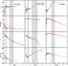 |
Fig. 6. Velocity dispersion, metallicity, age, and λR profiles for PGC007748 (left), PGC015524 (middle), and PGC049940 (right). The vertical dotted and dashed lines mark the position of the first and second transition radii, respectively. The gray shaded areas mark the transition regions between different components of the fit (see Sect. 5), and the red lines show the fit performed to estimate the slopes reported in Table 3. |
We also derived the total mass fraction (fh, T) enclosed in the second and third components of our fits. This is reported in Table 2. According to numerical simulation, this quantity has been suggested to be a proxy for the total accreted mass fraction, and it can be compared with the results of theoretical simulations as well as with other estimates for ETGs in the literature (as discussed in Sect. 6).
5. Results
The main aim of this section is to compare the observables we derived from the surface photometry (i.e., light and color distribution) with the stellar population properties derived from the spectroscopic analysis. In the bottom right panels of Figs. 1–3 we plot the azimuthally averaged (g − r) color profiles, and in Fig. 6 we plot the velocity dispersion, the luminosity-weighted metallicity and age, and the λR profile for the three galaxies we studied. The transition radii derived from the fit of the surface brightness profiles as well as the transition regions are also marked in the plots.
For PGC049940 the second transition radius occurs at R > 60 arcsec, that is, outside the galaxy regions covered by the MUSE field of view. For PGC007748 and PGC015524 instead, the first (Rtr1) and second (Rtr2) transition radii both lie within 60 arcsec.
The azimuthally averaged (g − r) color profiles show a similar behavior up to the first transition radius (Rtr2) for all the three galaxies (bottom panels of Figs. 1–3). They all have redder colors in the central regions. A gradient toward bluer colors is observed from the galaxy centers out to the first transition radius (Rtr1). For Rtr1 ≤ R ≤ Rtr2, the color profile of PGC007748 remains almost flat, while for PGC015524 it is slightly decreasing. The opposite occurs for the color profile of PGC049940, which shows a mild increase in the region Rtr1 ≤ R ≤ Rtr2. The three galaxies also differ in their outskirts. The color profile for PGC007748 is almost constant (g − r ∼ 0.8 mag) beyond Rtr2 up to ∼40 arcsec (R ∼ 0.7 arcmin, R/Re ∼ 1.5). Even if the slope of the color profile beyond Rtr2 is consistent with flat, the data indicate a trend for decreasing values toward bluer colors, g − r ≤ 0.7 mag at larger distances to the galactic center (R ≥ 0.7 arcmin). The outskirts of PGC015524 show steeper color gradients toward redder colors (g − r ∼ 0.8−0.9 mag) with respect to the average colors at smaller radii ≤100 arcsec (R/Re ≤ 2). The color profile in the outer regions of PGC049940 (R/Re ≥ 0.2) slightly increases toward redder colors (g − r ∼ 0.85−0.95 mag) despite the large error bars. For all the three galaxies, a discontinuity and a change in slope occurs in the color profiles at the transition regions.
Inside the first transition radius, the velocity dispersion (σ) decreases in both PGC007748 and PGC015524 (bottom row in Fig. 6). The σ profile for PGC049940 shows a drop in the center and a plateau, and then decreases at the first transition radius. For R ≥ Rtr1, σ still decreases in PGC007748 and PGC049940, whereas it shows a steeper positive gradient toward higher values (σ ∼ 280−330 km s−1) in PGC015524. In this galaxy, σ still grows in the outskirts at R ≥ Rtr2, being ∼350 km s−1 at R ∼ 1Re. In PGC007748, σ remains almost constant (∼220 km s−1) at R ≥ Rtr2.
The metallicity Z profiles have a different shape in the three galaxies (see the second row from the bottom in Fig. 6). In PGC007748, Z decreases with radius, with a steeper gradient observed for Rtr1 ≤ R ≤ Rtr2 and R ≥ Rtr2. The metallicity gradient is shallower in PGC015524 than observed in PGC007748 up to Rtr2, but we still observe a change in the slope at Rtr1 ≤ R ≤ Rtr2. In PGC049940, Z remains almost constant inside Rtr1 and decreases at R ≥ Rtr1, except for the strong change in the innermost regions (R/Re ∼ 0.02).
A similar behavior is found in the age profiles (see the third row from the bottom in Fig. 6). In PGC007748, age decreases with radius out to R ≃ Rtr1, it varies from ∼10 Gyr to 9.9 Gyr, and remains almost constant outward. In PGC015524, the stellar population age is about 10.12 Gyr at all radii. In PGC049940, age is almost constant at ∼10.1 Gyr for R ≤ Rtr1 and decreases to 9.9 Gyr at larger radii.
In the top panels of Fig. 6 we plot the λR parameter, which is a dimensionless parameter introduced by Emsellem et al. (2007) as a proxy for the baryon-projected specific angular momentum. We found that all three galaxies have very low λR and almost flat profiles (see Eqs. (12), (13), and (14) in Schulze et al. 2020), in agreement with their classification as slow rotators (Emsellem et al. 2011). For PGC007748, the λR profile slightly rises up to R/Re ∼ 0.1, while beyond this radius, it tends to flatten. The λR profiles for PGC015524 and PGC049940 are almost flat up to the second and first transition radius, respectively, where they show a peak. Beyond these radii, the λR profile for PGC015524 shows a mild increase, while the opposite occurs for PGC049940, which has a decreasing behavior.
In order to quantify the changes in the described profiles and correlate them with the transition radii from the photometry, we estimated the slopes5 of the profiles in three regions: R ≤ Rtr1, Rtr1 < R < Rtr2, and R ≥ Rtr2. The gradients of the metallicity, Δ [Z/H], and age, Δ Age, were derived by performing fits of the metallicity and age profiles plotted against log(R/Re). Following the definitions in Kuntschner et al. (2010), the metallicity and age gradients are defined as
![Mathematical equation: $$ \begin{aligned} \Delta \ [Z/H] = \frac{\delta \ [Z/H]}{\delta \ \log R/R_{e}} \end{aligned} $$](/articles/aa/full_html/2021/05/aa40186-20/aa40186-20-eq2.gif) (2)
(2)
 (3)
(3)
The derived values for surface brightness, metallicity, and age are reported in Table 3, and they are discussed in Sect. 6.
Logarithmic gradients of the surface brightness and metallicity and age profiles in three regions: R ≤ Rtr1, Rtr1 < R < Rtr2, and R ≥ Rtr2.
The analysis presented in this section suggests that there is a quite evident correlation between the color distribution, kinematics, and stellar population profiles. The transition radii set the scale of the different components in each galaxy.
6. Discussion: Observations (photometry and kinematics) versus simulations
6.1. Comparison with simulations and previous observational works
In this section we compare the results of the photometric and kinematic analysis with the prediction of theoretical simulations in order to trace the accretion history of the studied galaxies. As described in Sect. 4, by fitting the azimuthally averaged surface brightness distribution in the g band, we can proceed. When we assume that the last two components represent accreted stars, we can estimate their mass fraction (fh, T). Theoretical simulations predict that this quantity is a function of the total stellar mass in the galaxy; it is higher for massive galaxies (Cooper et al. 2013, 2015). First estimates of fh, T based on deep imaging are fully consistent with theoretical prescriptions (Seigar et al. 2007; Bender et al. 2015; Iodice et al. 2017b, 2020b; Spavone et al. 2017, 2018, 2020; Cattapan et al. 2019). In Fig. 7 we compare the values of fh, T derived for the three galaxies we studied with previous estimates. In agreement with previous theoretical and observational estimates, the outermost components in the galaxy light distribution account for most of the total galaxy stellar mass, in the range of 80%–90%.
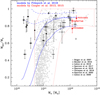 |
Fig. 7. Accreted mass fraction vs. total stellar mass for ETGs. Black symbols correspond to other BCGs from the literature (Seigar et al. 2007; Bender et al. 2015; Iodice et al. 2016, 2020b; Spavone et al. 2017, 2018, 2020; Cattapan et al. 2019), and red circles show galaxies in this work. The red region encloses the predictions of cosmological galaxy formation simulations by Cooper et al. (2013, 2015), which are indicated as gray dots. The continuous and dashed blue regions indicate the accreted mass fraction measured within 30 kpc and outside 100 kpc, respectively, in the Illustris simulations by Pillepich et al. 2018 (see their Fig. 12). |
In order to test the robustness of our estimate of the accreted mass fraction, as was done by Spavone et al. (2020), we examined how much this fraction is affected by leaving the Sérsic index free for the first component of the fit. We found that the Sérsic index ranges between 0.8 and 1, and that the accreted mass fractions change by 1%–3%, while the rms scatter does not change significantly.
Schulze et al. (2020) have recently used hydrodynamic cosmological Magneticum Pathfinder simulations to investigate the stellar kinematics of a sample of galaxies out to five half-mass radius6. Schulze et al. (2020) used the shape of the λR profiles of simulated galaxies to classify them. They reported three characteristic profile shapes: (i) decreasing profiles with a central peak at R ∼ 0.5−2Re and a decrease beyond this radius; (ii) increasing profiles that continuously increase out to the external regions, and (iii) flat profiles that remain almost flat over the whole radial range. According to Schulze et al. (2020), galaxies with decreasing λR profiles have a different accretion history than those with flat or increasing profiles. The former systems acquire most of the stellar mass through minor mergers, which is different from the galaxies with flat or increasing profiles, which build up from major mergers. In addition, Schulze et al. (2020) found that the radius marking the kinematic transition provides a good estimate of the transition radius between the in situ and accreted component in the photometric profiles. In particular, the peak of the λR declining profile corresponds to the transition radius between the in situ to ex situ component.
The λR profiles of galaxies in our sample are shown in the top panels of Fig. 6. According to the classification provided by Schulze et al. (2020), the three galaxies we studied have almost flat λR profiles and very low λmax. All the profiles rise slightly, and for PGC015524 and PGC049940, they show a peak corresponding to the second and first transition radius, respectively. The λR profile of PGC007748 increases up to just before first transition radius, then remains roughly constant, and the MUSE data show no decrease.
This means that all the studied galaxies are slow rotators in the range that we probe (Emsellem et al. 2007, 2011). Moreover, according to the predictions by Schulze et al. (2020), the region probed by MUSE indicates that the mass assembly occurred through major mergers (also supported by the velocity maps in Fig. 4, and see below), but we cannot rule out that minor mergers did not contribute in the outskirts. In particular, PGC049940 could be a good candidate for minor mergers based on the photometry. However, the MUSE data do not reach far enough out to probe the regions where the minor mergers would contribute the most, and therefore we do not know if λR would change according to the prescriptions by Schulze et al. (2020).
Additional clues on the formation pathways of investigated galaxies are found in the stellar velocity presented in Fig. 4 (and Krajnović et al. 2018). PGC007784 and PGC015524 are characterized by the prolate-like rotation (rotation around the major axis), while PGC0049940 has the more common rotation around the minor axis. If that prolate-like rotation is a consequence of major mergers (e.g., Li et al. 2018), the observed kinematics are consistent with the predictions by Schulze et al. (2020). Another interesting difference is found between PGC015524 and PGC049940, which also have detected emission-line gas (Pagotto et al. 2021). PGC15524 has a rather disturbed and filamentary gas distribution that extends to the edge of the MUSE field, while PGC049940 has a regular nuclear disk (within 2″). These observation may indicate that the assembly history of PGC049940 was somewhat different from that of the other two galaxies.
In the theoretical work by Cook et al. (2016), which is based on Illustris simulations, the authors performed a detailed analysis of the stellar halo properties of a sample of ETGs by studying their surface brightness, colors, and stellar populations. In particular, they addressed the accretion history of the simulated galaxies by studying the gradients of the above mentioned profiles in different galaxy regions, which are 0.1Re < R < 1Re (inner galaxy), 1Re < R < 2Re (outer galaxy), and 2Re < R < 4Re (stellar halo). The main conclusions of their work are that at fixed mass, the metallicity gradients and surface brightness profiles beyond 2Re are correlated with the amount of accreted mass, while the age and color gradients are poor indicators of the accretion history. In particular, tracing the assembly history of galaxies with time (since z = 1), Cook et al. (2016) found that the metallicity and surface brightness profiles tend to flatten as the accretion of metal-rich stars increases in the galaxy outskirts.
6.2. Interpretation of the results
Taking advantage of the long integration time and the large field of view of OmegaCam at VST, we were able to map the light distribution for the three galaxies we studied out to the regions of the stellar halos, that is, well beyond 2Re (∼4Re for PGC007748, ∼6Re for PGC015524, and ∼10Re for PGC049940). This is comparable with the theoretical predictions by Cook et al. (2016). The available integral field observations with MUSE cover only a limited portion (the brightest regions) of each galaxy (out to ∼1Re), and as a consequence, we cannot address any definitive conclusion on the relation between stellar population and accretion history in the galaxy outskirts. Because we were able to derive the first transition radius from the in situ to ex situ component, we can focus on these regions (i.e., R ≥ Rtr1) by fitting the surface brightness profiles in the following discussion.
The slopes of the surface brightness profiles are shallower in PGC015524 and PGC007748, and the slope is steeper in PGC049940 (see Fig. 5) and Table 3. According to Cook et al. (2016), as well as to Amorisco (2017), where the slope of the ex situ surface brightness profile depends on the total amount of accreted mass, we therefore expect that PGC015524 and PGC007748 have more accreted mass in their outskirts than PGC049940. This is indeed consistent with our independent estimate of the accreted mass fraction from the surface brightness distribution, where PGC015524 and PGC007748 have fh, T ∼ 86−89%, which is higher than the 77% derived for PGC049940 (see Table 2 and Fig. 7).
The flat λR profiles for all three galaxies also indicate that the great majority of the mass has been acquired through major mergers (Schulze et al. 2020). In the case of PGC007748 and PGC015524, this is consistent with the high fractions of accreted mass we estimated, as well as with steeper metallicity profiles beyond Rtr1. The limited extent of the spectroscopic data, however, does not constrain whether the outer halo of PGC049940 was built from major or minor mergers. This means that the lower accreted mass fraction (77%) for PGC049940, coupled with the steep surface brightness profile, might also indicate that its stellar halo is a result of minor mergers. Simulations predict that it is uncommon for a stellar halo to accrete a great amount of mass by minor mergers alone (Amorisco 2017; Cook et al. 2016).
7. Summary and conclusions
We have presented the new deep images from the VEGAS survey of three massive (M* ≃ 1012 M⊙) galaxies from the M3G project (Krajnović et al. 2018): PGC007748, PGC015524, and PGC049940. The long integration time and the wide field of view of OmegaCam at VST allowed us to map the light and color distributions down to μg ≃ 30 mag arcsec−2 and out to ∼2Re. At this depth and these distances, we were able to derive the contribution of the several components that dominate the galaxy light, in particular, the outer stellar envelope. By fitting the surface brightness distribution for each object, we estimated the accreted mass fraction that contribute to the ex situ component, and we compared this quantity with that predicted from simulations. The available integral field observations with MUSE cover a limited portion of each galaxy (the brightest regions out to ∼1Re), but from the imaging analysis, we found that they map the kinematics and stellar population beyond the first transition radius, where the contribution of the ex situ component starts to dominate.
The main goal of this work was to correlate the scales of the different components set from the images with the kinematics and stellar population profiles derived from the MUSE data. The results were combined to address the assembly history of the three galaxies with the help of the theoretical predictions. We summarise them below.
-
All three galaxies have a large amount of accreted mass in the range of 77% (for PGC049940) to 89% (for PGC015524). These high values are expected from simulations for galaxies of comparable stellar masses (M* ≃ 1012 M⊙). In addition, they are also consistent with the accreted mass fraction estimated from deep-imaging data available for other galaxies of similar masses (see Fig. 7).
-
As predicted by theoretical work from Schulze et al. (2020), a correlation exists between the shape of the λR profile with the transition radius from the in situ to ex situ components. In PGC007748 and PGC049940, this corresponds to the peak of the λR profile (see the top panels of Fig. 6). In PGC015524, the λR starts to increase slightly, and it reaches its highest value at the second transition radius (where the stellar envelope dominates the accreted component). The observed λR profiles are, however, mostly flat throughout the radial range of the MUSE data. Based on the Schulze et al. (2020) simulations, this suggests that the inner parts of galaxies were built through major mergers. Stellar velocity maps (Krajnović et al. 2018), in which PGC007748 and PGC015524 have prolate-like rotation, also support this evolutionary scenario. In the case of PGC049940, this might not be the entire picture because its velocity map is regular and a lower estimate of the accreted mass might indicate a less violent assembly history.
-
The gradients of the metallicity profile inside and outside the transition radii (i.e., for the in situ and ex situ components) are different for the three galaxies, as also shown by the change of slope in correspondence of the transition radii. In the region between the first and second transition radius we found no substantial differences between the metallicity gradients of the three galaxies. However, the ex situ component starts to be dominant outside the second transition radius. The only galaxy for which we can discuss gradients in this region is PGC007748. The metallicity and age profiles for PGC049940, in contrast, are not extended enough to cover the region of the second transition radius. For PGC015524 we only have a few points beyond Rtr2, and the gradients in this region are not reliable enough to draw conclusions. In the ex situ component of PGC007748, the metallicity profile tends to be flattened. The same behavior is observed in the surface brightness profile, indicating that more metal-rich stars are accreted in this galaxy. This correlation between the metallicity gradient and the surface brightness profile with the total amount of accreted mass is consistent with simulations by Cook et al. (2016).
All these results are combined in a coherent picture that traces the assembly history of the three galaxies we studied. PGC049940 has a lower accreted mass fraction (77%) than the other two galaxies. According to simulations by Schulze et al. (2020), at the range probed by MUSE data, the flat λR profile and its low amplitude indicate that the mass assembly in this galaxy was through major mergers. However, the steep surface brightness profile might indicate that the stellar halo in this galaxy is assembling by minor mergers (Amorisco 2017; Cook et al. 2016). For this reason, we cannot rule out that minor mergers did not contribute in the outskirts of PGC049940. The higher accreted mass fraction estimated for PGC007748 and PGC015524 and the flat λR profiles suggest that a great majority of the mass has been acquired through major mergers, which have also shaped the shallower metallicity profile observed at larger radii (R ≥ Rtr1). Moreover, these galaxies also have prolate-like velocity maps, which is most likely a consequence of a major merger on a radial orbit.
This work represents the first observational attempt to combine imaging and spectroscopy to trace the assembly history of massive galaxies. The deep images are crucial for mapping the light distribution down to the faintest regions of stellar halos and therefore to setting the scales of the main galaxy components. The results we obtained are encouraging. We therefore plan to acquire deep and more extended integral field data, which are needed to study the kinematics and stellar population content in the ex situ component.
IRAF (Image Reduction and Analysis Facility) is distributed by the National Optical Astronomy Observatories, which is operated by the Associated Universities for Research in Astronomy, Inc. under cooperative agreement with the National Science Foundation.
Available at http://purl.org/cappellari/software
See footnote 3 for availability.
For PGC049940, the innermost regions (R/Re ∼ 0.02) were excluded from the fit because the strong variations of both metallicity and age in these regions would affect the fit and lead to slopes that are not representative of the profiles.
The half-mass radius is considered to be equal to the effective radius Re.
Acknowledgments
We are very grateful to the anonymous referee for his/her comments and suggestions which helped us to improve and clarify our work. M.S. and E.I. acknowledge financial support from the VST project (P.I. P. Schipani). E.I. acknowledges financial support from the European Union Horizon 2020 research and innovation programme under the Marie Skodowska-Curie grant agreement n. 721463 to the SUNDIAL ITN network. DK and MdB acknowledge financial support through the grant GZ: KR 4548/2-1 of the Deutsche Forschungsgemeinschaft. Reduced MUSE cubes used in this work are available in the ESO science portal (http://archive.eso.org/scienceportal/home), while reduced VEGAS images will be ingested in the DR2 through the ESO phase 3.
References
- Abell, G. O., Corwin, H. G., Jr, & Olowin, R. P. 1989, ApJS, 70, 1 [NASA ADS] [CrossRef] [EDP Sciences] [Google Scholar]
- Amorisco, N. C. 2017, MNRAS, 469, L48 [NASA ADS] [CrossRef] [Google Scholar]
- Arnaboldi, M., Ventimiglia, G., Iodice, E., Gerhard, O., & Coccato, L. 2012, A&A, 545, A37 [NASA ADS] [CrossRef] [EDP Sciences] [Google Scholar]
- Arnold, J. A., Romanowsky, A. J., Brodie, J. P., et al. 2014, ApJ, 791, 80 [NASA ADS] [CrossRef] [Google Scholar]
- Bacon, R., Accardo, M., Adjali, L., et al. 2010, in Ground-based and Airborne Instrumentation for Astronomy III, SPIE Conf. Ser., 7735, 773508 [CrossRef] [Google Scholar]
- Barbosa, C. E., Arnaboldi, M., Coccato, L., et al. 2018, A&A, 609, A78 [NASA ADS] [CrossRef] [EDP Sciences] [Google Scholar]
- Barone, T. M., D’Eugenio, F., Colless, M., et al. 2018, ApJ, 856, 64 [NASA ADS] [CrossRef] [Google Scholar]
- Bender, R., Kormendy, J., Cornell, M. E., & Fisher, D. B. 2015, ApJ, 807, 56 [NASA ADS] [CrossRef] [Google Scholar]
- Cantiello, M., D’Abrusco, R., Spavone, M., et al. 2018, A&A, 611, A93 [NASA ADS] [CrossRef] [EDP Sciences] [Google Scholar]
- Capaccioli, M., Spavone, M., Grado, A., et al. 2015, A&A, 581, A10 [NASA ADS] [CrossRef] [EDP Sciences] [Google Scholar]
- Cappellari, M. 2017, MNRAS, 466, 798 [NASA ADS] [CrossRef] [Google Scholar]
- Cappellari, M., & Copin, Y. 2003, MNRAS, 342, 345 [NASA ADS] [CrossRef] [Google Scholar]
- Cappellari, M., & Emsellem, E. 2004, PASP, 116, 138 [NASA ADS] [CrossRef] [Google Scholar]
- Cattapan, A., Spavone, M., Iodice, E., et al. 2019, ApJ, 874, 130 [NASA ADS] [CrossRef] [Google Scholar]
- Coccato, L., Gerhard, O., Arnaboldi, M., et al. 2009, MNRAS, 394, 1249 [NASA ADS] [CrossRef] [Google Scholar]
- Coccato, L., Gerhard, O., Arnaboldi, M., et al. 2010, Highlights Astron., 15, 68 [Google Scholar]
- Coccato, L., Gerhard, O., Arnaboldi, M., & Ventimiglia, G. 2011, A&A, 533, A138 [NASA ADS] [CrossRef] [EDP Sciences] [Google Scholar]
- Coccato, L., Arnaboldi, M., & Gerhard, O. 2013, MNRAS, 436, 1322 [NASA ADS] [CrossRef] [Google Scholar]
- Cook, B. A., Conroy, C., Pillepich, A., Rodriguez-Gomez, V., & Hernquist, L. 2016, ApJ, 833, 158 [NASA ADS] [CrossRef] [Google Scholar]
- Cooper, A. P., Cole, S., Frenk, C. S., et al. 2010, MNRAS, 406, 744 [Google Scholar]
- Cooper, A. P., D’Souza, R., Kauffmann, G., et al. 2013, MNRAS, 434, 3348 [Google Scholar]
- Cooper, A. P., Parry, O. H., Lowing, B., Cole, S., & Frenk, C. 2015, MNRAS, 454, 3185 [Google Scholar]
- Deason, A. J., Belokurov, V., Evans, N. W., & Johnston, K. V. 2013, ApJ, 763, 113 [NASA ADS] [CrossRef] [Google Scholar]
- Donzelli, C. J., Muriel, H., & Madrid, J. P. 2011, ApJS, 195, 15 [NASA ADS] [CrossRef] [Google Scholar]
- Duc, P.-A., Cuillandre, J.-C., Karabal, E., et al. 2015, MNRAS, 446, 120 [Google Scholar]
- Emsellem, E., Cappellari, M., Peletier, R. F., et al. 2004, MNRAS, 352, 721 [NASA ADS] [CrossRef] [Google Scholar]
- Emsellem, E., Cappellari, M., Krajnović, D., et al. 2007, MNRAS, 379, 401 [Google Scholar]
- Emsellem, E., Cappellari, M., Krajnović, D., et al. 2011, MNRAS, 414, 888 [Google Scholar]
- Falcón-Barroso, J., Sánchez-Blázquez, P., Vazdekis, A., et al. 2011, A&A, 532, A95 [NASA ADS] [CrossRef] [EDP Sciences] [Google Scholar]
- Ferreras, I., Scott, N., La Barbera, F., et al. 2019, MNRAS, 489, 608 [Google Scholar]
- Fixsen, D. J., Cheng, E. S., Gales, J. M., et al. 1996, ApJ, 473, 576 [NASA ADS] [CrossRef] [Google Scholar]
- Foster, C., Arnold, J. A., Forbes, D. A., et al. 2013, MNRAS, 435, 3587 [NASA ADS] [CrossRef] [Google Scholar]
- Forbes, D. A., Gannon, J., Couch, W. J., et al. 2019, A&A, 626, A66 [NASA ADS] [CrossRef] [EDP Sciences] [Google Scholar]
- Forbes, D. A., Dullo, B. T., Gannon, J., et al. 2020, MNRAS, 494, 5293 [Google Scholar]
- Girardi, L., Bressan, A., Bertelli, G., & Chiosi, C. 2000, A&AS, 141, 371 [NASA ADS] [CrossRef] [EDP Sciences] [Google Scholar]
- Greene, J. E., Janish, R., Ma, C.-P., et al. 2015, ApJ, 807, 11 [NASA ADS] [CrossRef] [Google Scholar]
- Greene, J. E., Veale, M., Ma, C.-P., et al. 2019, ApJ, 874, 66 [NASA ADS] [CrossRef] [Google Scholar]
- Guérou, A., Krajnović, D., Epinat, B., et al. 2017, A&A, 608, A5 [NASA ADS] [CrossRef] [EDP Sciences] [Google Scholar]
- Hartke, J., Arnaboldi, M., Gerhard, O., et al. 2018, A&A, 616, A123 [NASA ADS] [CrossRef] [EDP Sciences] [Google Scholar]
- Huang, S., Leauthaud, A., Greene, J., et al. 2018, MNRAS, 480, 521 [NASA ADS] [CrossRef] [Google Scholar]
- Iodice, E., Capaccioli, M., Grado, A., et al. 2016, ApJ, 820, 42 [NASA ADS] [CrossRef] [Google Scholar]
- Iodice, E., Spavone, M., Cantiello, M., et al. 2017a, ApJ, 851, 75 [Google Scholar]
- Iodice, E., Spavone, M., Capaccioli, M., et al. 2017b, ApJ, 839, 21 [NASA ADS] [CrossRef] [Google Scholar]
- Iodice, E., Sarzi, M., Bittner, A., et al. 2019, A&A, 627, A136 [NASA ADS] [CrossRef] [EDP Sciences] [Google Scholar]
- Iodice, E., Spavone, M., Cattapan, A., et al. 2020a, A&A, 635, A3 [CrossRef] [EDP Sciences] [Google Scholar]
- Iodice, E., Cantiello, M., Hilker, M., et al. 2020b, A&A, 642, A48 [EDP Sciences] [Google Scholar]
- Jedrzejewski, R. I. 1987, MNRAS, 226, 747 [Google Scholar]
- Kormendy, J., Fisher, D. B., Cornell, M. E., & Bender, R. 2009, ApJS, 182, 216 [NASA ADS] [CrossRef] [Google Scholar]
- Krajnović, D., Cappellari, M., de Zeeuw, P. T., & Copin, Y. 2006, MNRAS, 366, 787 [NASA ADS] [CrossRef] [Google Scholar]
- Krajnović, D., Weilbacher, P. M., Urrutia, T., et al. 2015, MNRAS, 452, 2 [NASA ADS] [CrossRef] [Google Scholar]
- Krajnović, D., Emsellem, E., den Brok, M., et al. 2018, MNRAS, 477, 5327 [NASA ADS] [CrossRef] [Google Scholar]
- Kroupa, P. 2001, MNRAS, 322, 231 [NASA ADS] [CrossRef] [Google Scholar]
- Kuntschner, H., Emsellem, E., Bacon, R., et al. 2010, MNRAS, 408, 97 [NASA ADS] [CrossRef] [Google Scholar]
- Li, H., Mao, S., Emsellem, E., et al. 2018, MNRAS, 473, 1489 [NASA ADS] [CrossRef] [Google Scholar]
- Longobardi, A., Arnaboldi, M., Gerhard, O., et al. 2013, A&A, 558, A42 [NASA ADS] [CrossRef] [EDP Sciences] [Google Scholar]
- Lucy, L. B. 1974, AJ, 79, 745 [NASA ADS] [CrossRef] [Google Scholar]
- Ma, C.-P., Greene, J. E., McConnell, N., et al. 2014, ApJ, 795, 158 [Google Scholar]
- McDermid, R. M., Alatalo, K., Blitz, L., et al. 2015, MNRAS, 448, 3484 [NASA ADS] [CrossRef] [Google Scholar]
- McFarland, J. P., Verdoes-Kleijn, G., Sikkema, G., et al. 2013, Exp. Astron., 35, 45 [Google Scholar]
- Mihos, J. C., Harding, P., Feldmeier, J. J., et al. 2017, ApJ, 834, 16 [Google Scholar]
- Pagotto, I., Krajnović, D., den Brok, M., et al. 2021, A&A, 649, A63 [EDP Sciences] [Google Scholar]
- Pillepich, A., Nelson, D., Hernquist, L., et al. 2018, MNRAS, 475, 648 [NASA ADS] [CrossRef] [Google Scholar]
- Pulsoni, C., Gerhard, O., Arnaboldi, M., et al. 2020, A&A, 641, A60 [EDP Sciences] [Google Scholar]
- Pulsoni, C., Gerhard, O., Arnaboldi, M., et al. 2021, A&A, 647, A95 [EDP Sciences] [Google Scholar]
- Richardson, W. H. 1972, J. Opt. Soc. Am. (1917–1983), 62, 55 [Google Scholar]
- Sánchez-Blázquez, P., Peletier, R. F., Jiménez-Vicente, J., et al. 2006, MNRAS, 371, 703 [NASA ADS] [CrossRef] [Google Scholar]
- Saulder, C., van Kampen, E., Chilingarian, I. V., Mieske, S., & Zeilinger, W. W. 2016, A&A, 596, A14 [NASA ADS] [CrossRef] [EDP Sciences] [Google Scholar]
- Schipani, P., Noethe, L., Arcidiacono, C., et al. 2012, J. Opt. Soc. Am. A, 29, 1359 [Google Scholar]
- Schlafly, E. F., & Finkbeiner, D. P. 2011, ApJ, 737, 103 [NASA ADS] [CrossRef] [Google Scholar]
- Schulze, F., Remus, R.-S., Dolag, K., et al. 2020, MNRAS, 493, 3778 [CrossRef] [Google Scholar]
- Seigar, M. S., Graham, A. W., & Jerjen, H. 2007, MNRAS, 378, 1575 [NASA ADS] [CrossRef] [Google Scholar]
- Smette, A., Sana, H., Noll, S., et al. 2015, A&A, 576, A77 [NASA ADS] [CrossRef] [EDP Sciences] [Google Scholar]
- Spavone, M., Capaccioli, M., Napolitano, N. R., et al. 2017, A&A, 603, A38 [NASA ADS] [CrossRef] [EDP Sciences] [Google Scholar]
- Spavone, M., Iodice, E., Capaccioli, M., et al. 2018, ApJ, 864, 149 [NASA ADS] [CrossRef] [Google Scholar]
- Spavone, M., Iodice, E., van de Ven, G., et al. 2020, A&A, 639, A14 [CrossRef] [EDP Sciences] [Google Scholar]
- Spiniello, C., Napolitano, N. R., Arnaboldi, M., et al. 2018, MNRAS, 477, 1880 [Google Scholar]
- Trujillo, I., & Fliri, J. 2016, ApJ, 823, 123 [Google Scholar]
- Tully, R. B., Courtois, H. M., Dolphin, A. E., et al. 2013, AJ, 146, 86 [NASA ADS] [CrossRef] [Google Scholar]
- van de Sande, J., Bland-Hawthorn, J., Fogarty, L. M. R., et al. 2017, ApJ, 835, 104 [NASA ADS] [CrossRef] [Google Scholar]
- van Dokkum, P. G., & Conroy, C. 2010, Nature, 468, 940 [NASA ADS] [CrossRef] [Google Scholar]
- Vazdekis, A., Koleva, M., Ricciardelli, E., Röck, B., & Falcón-Barroso, J. 2016, MNRAS, 463, 3409 [Google Scholar]
- Veale, M., Ma, C.-P., Greene, J. E., et al. 2018, MNRAS, 473, 5446 [NASA ADS] [CrossRef] [Google Scholar]
- Venhola, A., Peletier, R., Laurikainen, E., et al. 2017, A&A, 608, A142 [NASA ADS] [CrossRef] [EDP Sciences] [Google Scholar]
- Venhola, A., Peletier, R., Laurikainen, E., et al. 2018, A&A, 620, A165 [NASA ADS] [CrossRef] [EDP Sciences] [Google Scholar]
- Weilbacher, P. M., Palsa, R., Streicher, O., et al. 2020, A&A, 641, A28 [CrossRef] [EDP Sciences] [Google Scholar]
All Tables
Logarithmic gradients of the surface brightness and metallicity and age profiles in three regions: R ≤ Rtr1, Rtr1 < R < Rtr2, and R ≥ Rtr2.
All Figures
|
Fig. 1. Left panel: VST color-composite gr image of the 20.7 arcmin × 19.4 arcmin field around PGC 7748. Top right panel: azimuthally averaged surface brightness profiles in the g (blue) and r (red) bands. Bottom right panel: azimuthally averaged (g − r) color profile. The vertical dotted and dashed lines mark the position of the first and second transition radii, respectively, and the gray shaded areas are the transition regions (see Sect. 5). |
| In the text | |
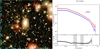 |
Fig. 2. Same as Fig. 1 for PGC 015524. The image size is 23.3 × 21.9 arcmin. |
| In the text | |
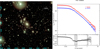 |
Fig. 3. Same as Fig. 1 for PGC 049940. The image size is 21.11 × 19.13 arcmin. |
| In the text | |
|
Fig. 4. Velocity, σ, metallicity, and age MUSE maps for the studied galaxies. The dashed black contours are isophotes. They are plotted in steps of half a magnitude. |
| In the text | |
|
Fig. 5. VST g-band profile of PGC007748 (top left), PGC015524 (top right), and PGC049940 (bottom) in linear scale, fit with a three-component model motivated by the predictions of theoretical simulations (see Spavone et al. (2017)). The bottom panels in each plot show the Δ rms scatter, obtained from the difference between the observed profiles (O) and the sum of the components from each fit (C). The dashed lines in all the panels indicate the galaxy cores. |
| In the text | |
|
Fig. 6. Velocity dispersion, metallicity, age, and λR profiles for PGC007748 (left), PGC015524 (middle), and PGC049940 (right). The vertical dotted and dashed lines mark the position of the first and second transition radii, respectively. The gray shaded areas mark the transition regions between different components of the fit (see Sect. 5), and the red lines show the fit performed to estimate the slopes reported in Table 3. |
| In the text | |
|
Fig. 7. Accreted mass fraction vs. total stellar mass for ETGs. Black symbols correspond to other BCGs from the literature (Seigar et al. 2007; Bender et al. 2015; Iodice et al. 2016, 2020b; Spavone et al. 2017, 2018, 2020; Cattapan et al. 2019), and red circles show galaxies in this work. The red region encloses the predictions of cosmological galaxy formation simulations by Cooper et al. (2013, 2015), which are indicated as gray dots. The continuous and dashed blue regions indicate the accreted mass fraction measured within 30 kpc and outside 100 kpc, respectively, in the Illustris simulations by Pillepich et al. 2018 (see their Fig. 12). |
| In the text | |
Current usage metrics show cumulative count of Article Views (full-text article views including HTML views, PDF and ePub downloads, according to the available data) and Abstracts Views on Vision4Press platform.
Data correspond to usage on the plateform after 2015. The current usage metrics is available 48-96 hours after online publication and is updated daily on week days.
Initial download of the metrics may take a while.