| Issue |
A&A
Volume 649, May 2021
|
|
|---|---|---|
| Article Number | A73 | |
| Number of page(s) | 16 | |
| Section | Extragalactic astronomy | |
| DOI | https://doi.org/10.1051/0004-6361/202039880 | |
| Published online | 13 May 2021 | |
The OTELO survey
Faint end of the luminosity function of [O II]3727 emitters at ⟨z⟩ = 1.43
1
Instituto de Astrofísica de Canarias (IAC), 38200 La Laguna, Tenerife, Spain
e-mail: bcedres@iac.es
2
Departamento de Astrofísica, Universidad de La Laguna (ULL), 38205 La Laguna, Tenerife, Spain
3
Instituto de Radioastonomía Milimétrica (IRAM), Av. Divina Pastora 7, Núcleo Central 18012, Granada, Spain
4
Asociación Astrofísica para la Promoción de la Investigación, Instrumentación y su Desarrollo, ASPID, 38205 La Laguna, Tenerife, Spain
5
Centro de Astrobiología (CSIC/INTA), 28692 ESAC Campus, Villanueva de la Cañada, Madrid, Spain
6
Instituto de Astronomía, Universidad Nacional Autónoma de México, Apdo. Postal 70-264, 04510 Ciudad de México, Mexico
7
Departamento de Física de la Tierra y Astrofísica, Instituto de Física de Partículas y del Cosmos, IPARCOS, Universidad Complutense de Madrid, 28040 Madrid, Spain
8
DARK, Niels Bohr Institute, University of Copenhagen, Lyngbyvej 2, Copenhagen 2100, Denmark
9
Instituto de Física de Cantabria (CSIC-Universidad de Cantabria), 39005 Santander, Spain
10
Instituto de Astrofísica de Andalucía, CSIC, 18080 Granada, Spain
11
ISDEFE for European Space Astronomy Centre (ESAC)/ESA, PO Box 78, 28690 Villanueva de la Cañada, Madrid, Spain
12
Instituto de Astronomía, Universidad Nacional Autónoma de México, 04510 Ciudad de México, Mexico
13
Fundación Galileo Galilei, Telescopio Nazionale Galileo, Rambla José Ana Fernández Pérez, 7, 38712 Breña Baja, Tenerife, Spain
14
Departamento de Física, Escuela Superior de Física y Matemáticas, Instituto Politécnico Nacional, 07738 Ciudad de México, Mexico
Received:
10
November
2020
Accepted:
25
February
2021
Aims. In this paper, we aim to study the main properties and luminosity function (LF) of the [O II]3727 emitters detected in the OTELO survey in order to characterise the star formation processes in low-mass galaxies at z ∼ 1.43 and to constrain the faint-end of the LF.
Methods. Here, we describe the selection method and analysis of the emitters obtained from narrow-band scanning techniques. In addition, we present several relevant properties of the emitters and discuss the selection biases and uncertainties in the determination of the LF and the star formation rate density (SFRD).
Results. We confirmed a total of 60 sources from a preliminary list of 332 candidates as [O II]3727 emitters. Approximately 93% of the emitters have masses in the range of 108 < M*/M⊙ < 109. All of our emitters are classified as late-type galaxies, with a lower value of (u − v) when compared with the rest of the emitters of the OTELO survey. We find that the cosmic variance strongly affects the normalisation (ϕ*) of the LF and explains the discrepancy of our results when compared with those obtained from surveys of much larger volumes. However, we are able to determine the faint-end slope of the LF, namely, α = −1.42 ± 0.06, by sampling the LF down to ∼1 dex lower than in previous works. We present our calculation of the SFRD of our sample and compare it to the value obtained in previous studies from the literature.
Key words: techniques: imaging spectroscopy / surveys / catalogs / galaxies: starburst / cosmology: observations / galaxies: luminosity function, mass function
© ESO 2021
1. Introduction
The luminosity function (LF) is a powerful tool used in characterising the distribution of star-forming galaxies at cosmological scales. By observing different emission lines, it is possible to trace the star-formation activity at different redshifts and, thus, at different epochs of the evolution of galaxies. Taking into account that the strongest emission line in a star-forming galaxy is usually Hα, this line can be considered the first probe for LFs (see e.g., Lilly et al. 1995, where their redshift sample ranges at 0 < z < 1.3; Geach et al. 2008 at z = 2.23; Sobral et al. 2013 at 0.40 < z < 2.23; Sobral et al. 2015 at z = 0.8; Khostovan et al. 2020 at z = 0.47; Ly et al. 2007 at 0.08 < z < 0.40; or more recently, Hayashi et al. 2020 at 0.09 < z < 0.48; and Harish et al. 2020 at z ∼ 0.62).
Other lines may be used when looking for other windows of observation in redshift, where Hα is not available. For example, the next most luminous line of the Balmer series, Hβ was employed for determining the LF at z ∼ 0.9 by Navarro Martínez et al. (2020). Other works have used the combination of Hβ and [O III], for example De Barros et al. (2019) reaching as far as z ∼ 8; Khostovan et al. (2015) up to 0.84 < z < 3.24; and Sobral et al. (2015) up to z = 1.4. In addition, there are a series of works were the LF is obtained by employing the doublet [O III]λλ 4959,5007 alone, for example, in Ly et al. (2007) at 0.41 < z < 0.84; Bongiovanni et al. (2020) at z ∼ 0.83; Khostovan et al. (2020) at 0.91 < z < 1.10; or Hayashi et al. (2020) at 0.05 < z < 0.94.
In order to sample the LF at very high redshift regimes, the Lyman α emitters are the objects of choice. For example, Ouchi et al. (2008), Sobral et al. (2018), and Herenz et al. (2019) obtained LFs at 3.1 < z < 5.7, 2 < z < 6, and 3 < z < 6, respectively.
Going back to intermediate redshift regimes, the [O II]λλ 3726,29 doublet, it is also a good candidate for the study of the LF. It is located in the bluemost part of the spectrum in rest frame, when compared with Hα, [O III]λλ 4959,5007, and Hβ, allowing us to reach larger values of the redshift from ground observations and avoiding the less transparent parts of the atmosphere in the infrared regime. The LF has been derived for this doublet by a number of authors who have employed spectroscopy or narrow-band techniques (Gallego et al. 2002 for the local universe; Khostovan et al. 2015 for 1.47 < z < 4.69; Khostovan et al. 2020 for 1.57 < z < 1.9; Drake et al. 2013 for 0.35 < z < 1.64; Ly et al. 2007 for 0.89 < z < 1.47; Comparat et al. 2015 for 0.1 < z < 1.65; or Hayashi et al. 2020 for 0.41 < z < 1.60). It has also been simulated from z = 0.1 to z = 3.0 by Park et al. (2015).
Nevertheless, at z > 1, the faint end of the [O II]3727 LF has not been properly observed. Indeed, almost all studies have no been capable of going beyond a log(L[O II]3727) ≃ 41 [erg s−1] in the best of cases (see e.g., the discussion in Khostovan et al. 2015). We believe that it is paramount to reach as low as possible in terms of luminosity in order to study the evolution of low-mass galaxies. For example, according to Sobral et al. (2011), the environment may be responsible for the slope of the faint end of the LF, being steeper for low-density regions and shallower for high-density fields. Moreover, the correct determination of the slope of the faint end of the LF influences the integration of the LF itself and, therefore, may vary the determination of the cosmic star formation history (SFH).
In this work, we take advantage of the sources detected in the OTELO survey (see Bongiovanni et al. 2019) to generate a catalogue of [O II]3727 emitters at z ∼ 1.43. We study the physical properties of these sources and we extend the study of the faint end of the LF for the [O II]3727 line to constrain the faint end slope and. In addition, we obtain the star formation rate density (SFRD) at this redshift.
The paper is organised as follows. In Sect. 2, we describe the OTELO survey and the selection of the sources. In Sect. 3, we present several of the derived properties from the data, including the extinction, the line fluxes, the morphology, and the stellar masses. In Sect. 4, we discuss the derived equivalent width of the emitters, in addition to studying a handful of high equivalent-width galaxies and comparing our results with those from the literature. Section 5 is devoted to our derived LF and the SFRD, along with a comparison with similar data from the literature. In Sect. 6, we summarise our main conclusions. For all the calculations carried out in this work, we assumed a standard ΛCDM cosmology with ΩΛ = 0.7, Ωm = 0.3, and h0 = 0.7.
2. The OTELO survey data and selection of the sources
2.1. The OTELO survey
In this work, we take advantage of the OTELO survey catalogue and its data products (for an in-depth description, see Bongiovanni et al. 2019). As a summary, the OTELO survey is a 2D spectroscopic blind survey covering a region of 56 arcmin2 of the Extended Groth Field. It has a resolution of R ∼ 700, covering a 230 Å of a selected atmospheric window (around 8950−9300 Å) that is relatively free of sky emission lines. The catalogue contains a total of 11237 sources and it is 50% complete at an AB magnitude of 26.38. From these sources, 5322 preliminary emission line candidates were selected according to the following criteria: (i) at least one point of the pseudo-spectrum lies above a value defined by fc + 2 × σc, where fc is the flux of the pseudo-continuum, defined as the median flux of the pseudo-spectra, and σc is the root of the averaged square deviation from fc of the entire pseudo-spectrum; and (ii) there is an adjacent point with a flux density above fc + σc (Bongiovanni et al. 2020).
The catalogue also presents complementary reprocessed data from several other surveys. This ancillary data covers from X-ray to far-infrared (FIR), both photometric and spectroscopic. Photometric redshifts (known as zbest) were determined through the LePhare code (Ilbert et al. 2006), using libraries for normal and starburst galaxies, QSOs, Seyferts and stars, and fitted to the OTELO photometric data. The zbest is designated as the z_BEST_deepY from Bongiovanni et al. (2019)1.
2.2. Selection of the sources
Taking into account that the [O II]λλ 3727,29 doublet must lie comfortably within the OTELO observing window of 8950−9300 Å, we selected, from the preliminary emission line candidates list, all the sources in the range of 1.40 < zbest < 1.50. Using this criteria, we selected a first subset of 332 emitters.
Following the work carried out by Bongiovanni et al. (2020) for the [O III]λ 4959,5007 emitters, and in order to produce a robust list of candidates, this first selection was visually screened by at least three researchers, looking for misidentifications, artifacts, and any other anomalies, such as truncated lines, overlapping sources, or multiple unlikely emission lines structures which appear in low signal-to-noise pseudo-spectra. From these cases, only those sources with truncated line in pseudo-spectra are considered true–positive emitters, despite their having been excluded from the final sample. However, this effect is included as a part of the sample completeness estimation described in Sect. 5.1. The resulting list was composed of 60 candidates. Table 1 summarises the classification determined for each one of the 332 candidates.
Classification summary of emission line candidates.
Employing the online tool developed for the OTELO database2, at least three researchers selected a new zguess by visual inspection that is closer to the real value of the redshift than the zbest. This zguess was employed as an input for the deconvolution program. To obtain the line fluxes from the pseudo-spectra, we employed the so-called inverse deconvolution, introduced in Cedrés et al. (2013) and developed in detail in Nadolny et al. (2020). Briefly, a series of simulations (on the order of 106) are performed and then a χ2 minimisation method is used to obtain the probability density function of the possible solutions for each source, taking the mode of the distribution as the best solution and the confidence intervals around the mode of all the associated parameters: fluxes, equivalent widths, redshifts, and continuum fluxes. In this paper, we quoted the uncertainties as the interval covering the 68% of such confidence interval. After all the candidates were deconvolved, a new visual inspection was carried out, this time to check the goodness of the fitted models. A catalogue with flux, equivalent width, redshift, and continuum flux was then generated. Following the deconvolution, zOTELO is derived from the OTELO pseudo-spectra for each emitter. This new redshift is a refinement of zguess.
Considering that we may have little contamination by AGNs due to our selection criteria in redshift (we only took galaxies fitted by a starburst or star-forming galaxies template), we decided not to correct for AGN contamination. Moreover, Drake et al. (2013) infer a contamination fraction about six percent in a sample of emitters at z = 1.6 and they suggest that AGN activity is usually associated with star-forming processes, so removing AGNs would lead to an over-correction.
We ran LePhare code a second time, but with redshift fixed to zOTELO and restricted to star-forming galaxies templates with the aims of obtain a more accurate value of reddening. The applied galaxy templates are Kinney et al. (1996) and Bruzual & Charlot (2003) – with a continuous star formation law.
One example of a deconvolved pseudo-spectrum is shown in Fig. 1. Even if the source is noisy, the fitted model is good enough to extract the required information. On the other hand, in Fig. 2, we represent the pseudo-spectrum and deconvolving lines for an object with a much better signal-to-noise ratio (emitter id:8532). In Fig. A.1 in the appendix, we represent the pseudo-spectra of all selected emitters in the catalogue.
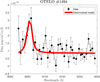 |
Fig. 1. Pseudo-spectra and deconvolved spectra for the id:1494 emitter. We note the noisy aspect of the pseudo-spectra. However, in these circumstances, the model is capable of obtaining a good measure of the [O II]3727 lines. |
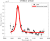 |
Fig. 2. Pseudo-spectra and deconvolved spectra for the id:8532 emitter. The signal-to-noise ratio is better than in Fig. 1. |
3. Derived properties
3.1. Extinction correction
The obtained fluxes were corrected via internal extinction following the law presented in Calzetti et al. (2000) and employing the reddening E(B − V) obtained as an output from the second fitting of the emitters using the LePhare code (see Bongiovanni et al. 2019). We also took into account the inherent extinction of the templates in Kinney et al. (1996) when deriving our value for the extinction.
In Fig. 3, we have represent the histogram of the derived value of A[O II]3727 for all the emitters. The mean result is ⟨A[O II]3727⟩ = 0.88 mag, which is equivalent to ⟨AHα⟩ = 0.5 mag, with a standard deviation of σ = 0.5. This is lower than the normally employed AHα ∼ 1 mag. This value has been experimentally obtained, for example, by Ibar et al. (2013), who reported an AHα = 1.0 ± 0.2 mag for objects at z = 1.47, employing a combination of far-IR and Hα data. On the other hand, our result seems to agreed with the trend observed in other works and cited in Hayashi et al. (2013), where the authors found that [O II]3727 emitters selected by narrow-band (NB) techniques are likely to be dust-poor systems. For example, both Hayashi et al. (2013) and Khostovan et al. (2020) give AHα ∼ 0.35 mag for emitters at z ∼ 1.47, Hayashi et al. (2015) found AHα = 0.63 mag for z = 1.5, and Khostovan et al. (2015) obtains AHα = 0.55 ± 0.12 mag for emitters at z = 1.59. Nevertheless, the large dispersion of the mean value derived makes difficult to obtain a clear conclusion about the absorption nature of our emitters. As Garn et al. (2010) have pointed out, the individual extinctions vary significantly between galaxies, which is clearly visible in the histogram of Fig. 3.
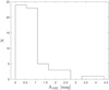 |
Fig. 3. Histogram of the value of A[O II]3727 for all the emitters in the catalogue. |
3.2. Line fluxes
In Fig. 4, we represent the histogram of the measured flux for all the emitters, corrected for extinction. The lowest flux is log(f[O II]3727 min) = −17.72 [erg cm−2 s−1], the maximum is log(f[O II]3727 max) = −15.56 [erg cm−2 s−1], and the mean value is ⟨log(f[O II]3727)⟩ = −17.02 [erg cm−2 s−1]. We can observe that only the 15% of the emitters have a flux higher than log(f[O II]3727) = − 16.75 [erg cm−2 s−1].
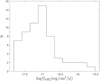 |
Fig. 4. Histogram of the line flux (extinction corrected) observed for all the selected emitters. |
3.3. Morphology
Following Kauffmann et al. (2003), we define the concentration index C as the ratio of the radius enclosing the 90% of the luminosity in a defined band over the radius enclosing the 50% of the luminosity in the same band. In our case, we employed the high-resolution images from the bands F814W(I) and the F606W(V) from HST/ACS. However, only 45 emitters from our sample had data in those filters. The median value for the I filter is CI = 1.92. However, as shown, for example, in Strateva et al. (2001) and in Nadolny et al. (2021), this parameter may only serve to establish a crude classification between early-type (ET) and late-type (LT) galaxies.
In Nadolny et al. (2021) the intensity spatial distribution of the emitters from the OTELO survey is fitted using a parametric form in a Sersic (1968) profile, defined as:
![$$ \begin{aligned} I(r) = I_{\rm e} \exp \{-b_{n}[(r/r_{\rm e})^{1/n} - 1]\}, \end{aligned} $$](/articles/aa/full_html/2021/05/aa39880-20/aa39880-20-eq1.gif)
where re is the effective radius (i.e. radius containing 50% of total flux), Ie is the intensity at re in the filter selected (F814W or F606W from HST/ACS in this case), n is the Sérsic index, and bn is a function of n as defined in Ciotti (1991). For a detailed description of the fitting process, see Nadolny et al. (2021). The obtained Sérsic index n is an useful tool in order to classify the morphology of the emitting sources. For disc-dominated LT galaxies, the expected value of this parameter in the I filter is nI < 4 (Nadolny et al. 2021). The median values obtained for the [O II]3727 emitters is nI = 2.1 ± 1.7. This value appears to be slightly larger than the mean value obtained for all the emitters with enough data for the OTELO survey Nadolny et al. (2021) (nI = 1.3). However most of the emitters show nI values below the threshold for LT galaxies. On the other hand, our results are well within the range obtained by Paulino-Afonso et al. (2017), who give  for the emitters at z = 1.47 from High-Z Emission Line Survey (HiZELS).
We also derived the ratio of Sérsic indices in both bands  introduced by Vika et al. (2015). This parameter is sensitive to the internal structure of the galaxy when paired with a colour term. In this case, the median value obtained was
  , which is well inside the error margin for the whole OTELO database, where the value was
  for the LT galaxies (Nadolny et al. 2021). In Fig. 5, we reproduce the results from Nadolny et al. (2021).
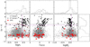 |
Fig. 5. Observed (u − r) colour versus morphological parameters for all the sources of OTELO. From left to right: logarithm of the Sérsic index in the filter F814W (I), concentration index for the I filter too, and the logarithm of the wavelength-dependent ratio of the Sérsic indices for I and V (F606W). Triangles and solid lines in grey (histograms) represent LT, squares and dashed lines in black (histograms) represent ET galaxies. Red circles represent the [O II]3727 emitters from our sample with HST/ACS ancillary data. Top histograms corresponds to the respective value, as indicated in x-axis label, while right-hand histogram show (u − r) distribution. All histograms represents density distributions. Horizontal dot-dashed line in black shows (u − r) = 2.5. Red dashed line shows the results from de Diego et al. (2020). Dashed lines in magenta represent limits from Vika et al. (2015): horizontal cut in (u − r) = 2.3, while vertical dashed-lines in magenta represent log(nI) = 0.4 and |
The red dashed line marks the linear discriminant analysis developed by de Diego et al. (2020), employing deep learning methods for morphology classification. In the figure we can see that all the selected emitters (indicated by red circles) are comfortably distributed in the late-type locus. Moreover, almost all detected emitters are somewhat bluer than the mean of the all OTELO ET galaxies.
3.4. Derived masses
Following López-Sanjuan et al. (2012) we obtained an estimation of the stellar mass for 48 of the emitters in the catalogue (for a detailed description of the process, see Bongiovanni et al. 2020). The remaining 12 emitters with no stellar mass determination presented a large error in several of the ancillary bands that made it impossible to derive a meaningful value for the mass.
The median value derived for the stellar mass was log (M*/M⊙) = 8.87, with a dispersion of log (M*/M⊙) = 0.67. The largest mass derived was log (M*/M⊙) = 10.93, meanwhile, the lowest mass was log (M*/M⊙) = 7.89. If we define the low-mass population as the galaxies with M* < 1010 M⊙ (Bongiovanni et al. 2020), only three emitters present are out of the low-mass regime. This means that about 93% of the emitters belong to the low-mass criterion. In Bongiovanni et al. (2020), the percentage of low-mass galaxies reached 87% in a catalogue composed by 171 emitters at a ⟨z⟩ = 0.83; meanwhile for Nadolny et al. (2020), the whole sample of Hα emitters was in the low-mass regime, with a 63% being very low-mass galaxies (M* < 109 M⊙). These two results seems compatible with the stellar masses derived in our sample, indicating that the OTELO survey favours the detection of low-mass galaxies. This is a direct consequence of an ultra-deep pencil-beam designed survey, as the OTELO survey is, in fact (Bongiovanni et al. 2019). The mass distribution for the emitters is represented in Fig. 6.
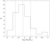 |
Fig. 6. Histogram of the derived stellar mass (in solar masses) for the emitters. The dashed line marks the position of the median value at log (M*/M⊙) = 8.87 and the point-dashed lines mark ±1σ over the median value. |
4. [O II]3727 Equivalent width
One of the parameters derived from the deconvolution is the equivalent width of the [O II]3727 doublet. In Fig. 7, we represent the histogram of the logarithm of EW[O II]3727. The minimum value obtained in our emitters is 10 ± 5 Å and the maximum is 185 ± 16 Å. The median value is EW[O II]3727 = 65 Å, with a 1σ dispersion of EW[O II]3727 = 37 Å. Following Ramón-Pérez et al. (2019), in EWHα, the minimum value for detection with a probability p ≤ 0.95 was ∼10.5 Å. In order to estimate our detection limit, we have to translate our limit in EWHα into a limit in EW[O II]3727. For this reason, we can employ the relationship given by Kennicutt (1992), which is summarised in Eq. (2):
![$$ \begin{aligned} {\mathrm{EW}_{[{\text{ O}}{\small {{\text{II}}}}]3727}}=0.4\times {\mathrm{EW}_{(\mathrm{H}\alpha +[{\text{ N}}{\small {{\text{II}}}}])}}. \end{aligned} $$](/articles/aa/full_html/2021/05/aa39880-20/aa39880-20-eq7.gif)
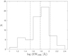 |
Fig. 7. Histogram of the line equivalent width for all the selected [O II]3727 emitters in OTELO. The dashed line marks the position of the median value, and the point dashed lines mark ±1σ over the median value. |
However, this relationship was obtained for nearby galaxies and it also presents a large dispersion for galaxies with very strong emission lines. Nevertheless, employing Lamareille et al. (2006) data, we were able to calculate this relationship for galaxies with 0.2 < z < 1.0. In this case, the resultant slope was 0.5 ± 0.1, very similar to the 0.4 value from Kennicutt (1992) relationship. Based on this premise, the minimum value we would be able to detect with p ≤ 0.95 is ∼4.2 Å. In this case, it is clear that all our emitters are well over this threshold.
In Huang et al. (2015), several galaxies with high equivalent width in the [O III]λ5007 (> 3000 Å at restframe) lines are studied. They found that those galaxies can be classified as: low-mass, strong starbust, and compact. Following the models of Villaverde et al. (2010), we can assume a maximum equivalent width of the [O II]3727 line for ‘normal’ galaxies at 150 Å. Indeed, Kong et al. (2002) found that galaxies with EW[O II]3727 > 100 Å are in the 90th percentile and Thomas et al. (2013), based on data from the SDSS-III/BOSS, showed that galaxies with EW[O II]3727 > 100 Å are located outside the limits of their figures. Being conservative, we can then select for our galaxies a minimum value for high equivalent width galaxies at ∼150 Å.
Based on a first approximation, taking into account the models presented in Villaverde et al. (2010), those high equivalent-width galaxies in [O III]λ5007 may be an analogous to our detected emitters with high [O II]3727 equivalent width.
In Table 2, we summarise the properties of the emitters with high [O II]3727 equivalent width. We note we include emitter id:3345, with EW[O II]3727 = 140 Å. This is smaller than the selected value of 150 Å, however, the error in the equivalent width associated with this emitter makes it compatible with a galaxy with high equivalent with in [O II]3727.
Emitters with high [O II]3727 equivalent width.
The emission at the line [O II]3727 is influenced by metallicity and the star formation history (see e.g., Anders & Fritze-v. Alvensleben 2003). It was also noted in Villaverde et al. (2010) that EW[O II]3727 presents an important mass and metallicity dependence for ages lower than ∼4.5 Myr, and with no dependence at older ages. On the other hand, the EW[O III]5007 has a negligible dependence with the mass. For this reason, a region with large EW[O II]3727 may not simultaneously have a large EW[O III]5007, and they may not be the same type of object. From Table 2, it is clear that the emitters id:3077 and id:8532 have both masses that put them in the low-mass galaxy regime. Moreover, we have complete morphology data for emitter id:8532 and it seems to point out towards a disc-like emission galaxy. This may also indicate also that a high [O III] equivalent-width objects are not the same type of emitters as the ones with high [O II]3727 equivalent width. Unfortunately, we do not have enough information to establish the correct morphology for all our emitters nor their masses. Nevertheless, we are able to establish a upper limit for the masses of id:3345 and id:6445, both of them well inside the low-mass regime. In Fig. 8 we have represented the cutouts for the emitters with high [O II]3727 equivalent width in the composite OTELO band, obtained by adding all the slices of the scan (see Bongiovanni et al. 2019 for an in-depth description).
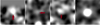 |
Fig. 8. Thumbnails in the OTELO composite filter (obtained adding all the slices of the scan) for the sources with high equivalent width. The red arrow indicates the location of the source. Each thumbnail has 8 × 8 arcsec size. From left to right: id:3077, id:3345, id:6445, and id:8532. |
In Fig. 9, we represent the [O II]3727 equivalent width in Å versus the logarithm of the derived mass of our emitters. We stacked our data in bins of 0.5 dex and we added data from other authors: (Paulino-Afonso et al. 2020, P-A20) with galaxies z ∼ 0.8, (Darvish et al. 2015, D15) with z ∼ 0.5, and Reddy et al. (2018) with z ∼ 1.5. We also fitted a simple function using least squares to the data in the form of the following equation:
![$$ \begin{aligned} {\mathrm{EW}[{\text{ O}}{\small {{\text{II}}}}]3727}=p_1 \times \log ({M_*/{M_{\odot }}})+p_2. \end{aligned} $$](/articles/aa/full_html/2021/05/aa39880-20/aa39880-20-eq9.gif)
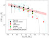 |
Fig. 9. Relationship between the [O II]3727 equivalent width and the derived stellar mass for our emitters (cyan open circles). The black diamonds are the median of our emitters for bins 0.5 dex in log(M*/M⊙), and the data from Paulino-Afonso et al. (2020) (red closed squares), Darvish et al. (2015) (filled purple stars for filament galaxies and green triangles for field galaxies), and Reddy et al. (2018) (grey diamonds). The black dashed line represents the best fit for all the binned data and the cyan point-dashed line represent the best fit for the only the binned data of the emitters detected in this work. The pink band represents the power law fit with uncertainties from Khostovan et al. (2016) for [O II]3727 emitters at z = 1.47. |
The results of the fitting are given in Table 3 and we also represent the fit obtained from Khostovan et al. (2016) for the [O II]3727, emitters at z = 1.47, with its uncertainties, as a pink band. This fit is a power law with the form EW![$ _{{[{\mathrm{O}\,\textsc{II}}]3727}}=k\times M_*^{\beta} $](/articles/aa/full_html/2021/05/aa39880-20/aa39880-20-eq10.gif) , where β = −0.23 and log(k) = 3.79. As pointed out by Paulino-Afonso et al. (2020), higher stellar mass galaxies have lower equivalent widths in [O II]3727, independently of the environment. They suggest that this trend is mostly a consequence of the underlying main sequence of star-forming galaxies. Our data seems to follow this behaviour. On the other hand, there is a large difference between our data and those of Paulino-Afonso et al. (2020) at higher stellar masses. We must point out that we are sampling lower-mass galaxies than Paulino-Afonso et al. (2020), Darvish et al. (2015), and Reddy et al. (2018). On the other hand, Reddy et al. (2018) seem to have a large value for the equivalent width when compared with other authors (Paulino-Afonso et al. 2020; Darvish et al. 2015), but their results are inside the error margins of ours – and this is not surprising. As Khostovan et al. (2016) have shown, there is also a dependence of the EW[O II]3727 with the redshift, with larger values for EW[O II]3727 when increasing z, up to z ∼ 4, followed by a decreasing of the equivalent width at higher redshifts. This may be the reason for the lower value of EW[O II]3727 at high stellar masses obtained in Paulino-Afonso et al. (2020), as well as in Darvish et al. (2015), when compared with those presented in Reddy et al. (2018), Khostovan et al. (2016), and this work.
, where β = −0.23 and log(k) = 3.79. As pointed out by Paulino-Afonso et al. (2020), higher stellar mass galaxies have lower equivalent widths in [O II]3727, independently of the environment. They suggest that this trend is mostly a consequence of the underlying main sequence of star-forming galaxies. Our data seems to follow this behaviour. On the other hand, there is a large difference between our data and those of Paulino-Afonso et al. (2020) at higher stellar masses. We must point out that we are sampling lower-mass galaxies than Paulino-Afonso et al. (2020), Darvish et al. (2015), and Reddy et al. (2018). On the other hand, Reddy et al. (2018) seem to have a large value for the equivalent width when compared with other authors (Paulino-Afonso et al. 2020; Darvish et al. 2015), but their results are inside the error margins of ours – and this is not surprising. As Khostovan et al. (2016) have shown, there is also a dependence of the EW[O II]3727 with the redshift, with larger values for EW[O II]3727 when increasing z, up to z ∼ 4, followed by a decreasing of the equivalent width at higher redshifts. This may be the reason for the lower value of EW[O II]3727 at high stellar masses obtained in Paulino-Afonso et al. (2020), as well as in Darvish et al. (2015), when compared with those presented in Reddy et al. (2018), Khostovan et al. (2016), and this work.
Cava et al. (2015) studied two groups of [O II]3727 emitters: one at z ∼ 0.84 and other at z ∼ 1.23. They reached a result a bit below log(M*/M⊙) < 9, while for z ∼ 1.23 and at low mass galaxies, there is little correlation between the equivalent width and the derived stellar mass. This is similar to our results for the non-stacked and stacked sources at low stellar mass. On the other hand, at z ∼ 0.84, Cava et al. (2015) found a clear correlation between the masses and the equivalent width as that presented in Paulino-Afonso et al. (2020), down to log(M*/M⊙)≃8.5). This discrepancy may be due to the low number of sources detected at larger redshifts, so we may assume that the correlation should appear with a set of enough emitters. Nevertheless, our results closely follow the fit from Khostovan et al. (2016) down to log(M*/M⊙)< 8.5, even when Khostovan et al. (2016) data has few galaxies below that threshold. Moreover, if we calculate the exponent β for our binned data, we obtain β = −0.20 ± 0.04, which agrees, within uncertainties, with the one obtained in Khostovan et al. (2016), β = −0.23 ± 0.01.
5. The [O II]3727 luminosity function
Using the data obtained for all the emitters in the catalogue, we derived the LF for the [O II]3727 line emitters at z ∼ 1.43 after taking into account the main sources for uncertainties and selection effects: the completeness of the sample and the cosmic variance (CV).
5.1. Completeness
To correct for completeness, we have followed the methods described in Bongiovanni et al. (2020). To summarise, several simulations were carried out to calculate the detection probability function from emission-line sources in the OTELO survey. These simulations helped to calibrate the detection probability as a function of the [O II]3727 line flux. This probability function was then fitted by a sigmoid algebraic function (Eq. (4)).
where d is the fitted mean detection probability, F = log(f[O II]3727) + b, and a = 0.961 ± 0.010, b = 18.297 ± 0.032, c = 0.660 ± 0.099 are the fitted parameters. In Fig. 10, we show the completeness correction function and the mean detection probability for the emitters at z ∼ 1.43.
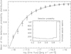 |
Fig. 10. Mean of the detection probability of the [O II]3727 emitters at ⟨z⟩∼1.43. As described in Bongiovanni et al. (2020), the inset shows the detection probability distribution obtained from the simulations. The curve represents the least-square weighted fit of the sigmoid function. The bars indicated the mean standard error. |
5.2. Cosmic variance
The comoving volume covered by OTELO at the redshift of this catalogue is about ∼1.0 × 10⁴ Mpc3, along with an explored sky area of about 0.015 deg2. Because of this small volume (when compared with other surveys; see Table 3), the effects of CV are remarkable. Indeed, Stroe & Sobral (2015) found that volumes smaller that 3 × 10⁴ Mpc3 are affected in such a way for CV that the results in the determination of the LF could lead to errors up to 100% in the parameters employed to fit the such LF. This is confirmed in Ramón-Pérez et al. (2019), where it was derived a global root of the CV of σv ≃ 0.73, based on the prescription of Somerville et al. (2004), for a comoving volume of 1.4 × 10³ Mpc3 and a redshift of z ∼ 0.40. And in Bongiovanni et al. (2020), for a mean volume of 6.63 × 10³ Mpc3 and a a sample of objects at z ∼ 0.83, the root CV obtained was σCV = 0.396, by using the code3 described in Moster et al. (2011). It is thus made clear that obtaining an estimation of the CV is a necessary condition if we want to correctly characterise the [O II]3727 luminosity function.
According to the mean number density of [O II]3727 line emitters (1.4 × 10⁻³ Mpc−3), it is expected that the CV effects are more pronounced than the estimated for previous OTELO samples at lower redshifts, despite the increased cosmic volume explored at z ∼ 1.43 as compared to those cases. On this basis, we examined the contribution of the CV to the uncertainty of the LF from each approach used in the OTELO papers referred above. On one side, Somerville et al. (2004) provide a recipe to estimate the CV based on a known average redshift and number density in deep surveys, but unknown clustering strength. The mean root CV obtained for the science case presented here is σv ≃ 0.61. On the other hand, the approach given by Moster et al. (2011) allows us to compute CV as a function of mean redshift, redshift bin size, and the stellar mass of the subject galaxy population. By following this prescription, we were able to estimate an uncertainty function attributed to the CV, σCV(M⋆) for six bins in the stellar mass range 8.5 ≤ log(M⋆/M⊙) ≤ 11.5 for the [O II]3727 sample, and the mean uncertainty obtained for our sample at ⟨z⟩ = 1.43 is ⟨σCV⟩ = 0.304. In view of the noticeable difference between these estimations, we decided to adopt the Somerville et al. (2004) recipe for being the most conservative one. In the final part of Sect. 5.3, we further discuss the reliability of this approach for the science case presented in this work.
5.3. [O II] luminosity function
The LF computes the number of galaxies (ϕ) per unit of volume and per unit of luminosity. The Schechter (1976) function is the usual parameterisation method:

where L is the luminosity of the emission line ([O II]3727 in our case), ϕ* is the density number of galaxies, L* is the characteristic luminosity, and α defines the faint-end slope of the LF.
The value of ϕ was calculated according to Bongiovanni et al. (2020) as follows:
![$$ \begin{aligned} \phi [\log L([{\text{ O}}{\small {{\text{II}}}}]3727)]= \frac{4\pi }{\Omega }\Delta [\log L([{\text{ O}}{\small {{\text{II}}}}]3727)]^{-1}\sum _{i} \frac{1}{V_{i} d_{i}}, \end{aligned} $$](/articles/aa/full_html/2021/05/aa39880-20/aa39880-20-eq13.gif)
where di is the detection probability for the ith galaxy, obtained with Eq. (4), Vi is the comoving volume for the ith source, Ω is the surveyed solid angle (∼4.7 × 10⁻⁶ str), and Δ[log L([O II]3727)] = 0.4 is the adopted luminosity binning.
The [O II]3727 luminosities based on extinction-corrected line fluxes (Sect. 3) were sampled in seven bins distributed in the range 40.13 < log L([O II]3727) < 42.93. For each bin, ϕ values were obtained using Eq. (6). The total uncertainty of each value mainly come from the quadratic combination per luminosity bin of the Poisson error obtained from the number of galaxies, which mean contribution is about 40% (increasing from a 23% for lower luminosity bins up to 70% for the upper-side bin) and the uncertainty associated with the CV. Following the recipe provided by Somerville et al. (2004), the estimated root of the CV, σv, increases from 0.6 at the log L([O II]3727) = 40.33 bin, to 0.91 at the log L([O II]3727) = 42.73 one. Total uncertainty in each bin also includes the contribution of the mean standard error of the completeness correction (Sect. 5.1) and the probability of incorrect emission-line sources identification (which also includes the fraction of bona fide emitters lost) based on Bongiovanni et al. (2020), amounting together to ∼6%. The resulting uncertainties from such combinations, along with the LF data are given in Table 4.
In Table 5, we summarise the Schechter parameters derived for the fit of the LF, as well as the parameters for other works at similar redshifts and with the [O II]3727 line (Drake et al. 2013; Ly et al. 2007; Hayashi et al. 2013). The Schechter model function of Eq. (5) was fitted to the data given in this table using a weighted least-squares minimisation algorithm based on the Levenberg–Marquardt method4. Weights are defined as the reciprocal of the squared total uncertainties of LF data.
We used a fixed value for log L* obtained as the average of the well-known values from the works presented in Table 5, that is, log L* = 42.44, with a standard deviation of σ = 0.09. This was done because our sampling over log(L*)≳42.5 is poor, and consequently, log L* is completely unconstrained in the fitting process. Assuming this standard deviation as a measure of the log L* uncertainty and that it is normally distributed, we estimated the standard errors of the fitted parameters ϕ* and α from 105 realisations of the fitting procedure described above. The uncertainties thus obtained amount 50.3% and 4.2% of the fitted ϕ* and α values. Due to the limited cosmic volume explored by OTELO, large variances would be expected in the normalisation of the LF after fitting, as confirmed by the error estimate of ϕ*. The opposite occurs with the uncertainty linked to the faint-end slope of the LF since our sample extends far beyond the lower limits reached by other, similar surveys.
In Fig. 11, we represent the LF data for our emitters and their best fittings. The bin with the lowest luminosity (log L([O II]3727) = 40.33 [erg s−1]) and marked with an open circle, has not been included in the calculations because the method employed to derive the completeness underestimates the number of emitters in the bin, so the errors there are also underestimated. It is clear that our data (represented as black dots) has a lower value for log ϕ at lower luminosities when compared with other works. Consequently, our value of ϕ* is lower when it is set against those presented in Table 5, and it is a clear effect of the uncertainties on the CV. Nevertheless, as pointed out in Drake et al. (2013), the detection fraction of emitters is very sensitive to the limit of equivalent width in a NB survey, which is of the order of the filter width. So, in this case, as noted in the discussion of Bongiovanni et al. (2020), the lower limit of equivalent width with OTELO survey is about 6 Å, which is lower than those obtained by the classic narrow-band studies. There, the lower limit for the equivalent width can be over 50 Å, depending on the technique. This fact comparatively favours the detection of low-mass emitters, despite the CV effects.
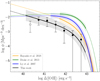 |
Fig. 11. Luminosity function for the [O II]3727 emitters at z ∼ 1.43 (black circles), with extinction and completeness corrected. The error bars correspond to the total uncertainties given in Table 4, and obtained as described in the text. The open circle marks the lowest luminosity bin and was not employed in the fitting. The black line is the best error-weighted fit of Schechter (1976) function. The green, blue, and orange lines are the LFs from Drake et al. (2013), Ly et al. (2007), and Hayashi et al. (2013) respectively. The shaded areas represent the propagation of 1σ uncertainties of the tabulated LF after 104 Monte Carlo realisations. For the OTELO data fitting, this propagation includes the standard deviation of the mean L* value. In each case, the solid line extend over the sampled luminosity range (see the right side columns in Table 4) and the dashed line is the extrapolation of the corresponding best fit. |
It is also worthwhile noting that we sampled the faint end of the LF by almost one dex lower when compared with other authors. We obtained a value for α equals to −1.42 ± 0.06. This result is similar to that reported by Hayashi et al. (2013), but different from those reported in Drake et al. (2013) and Ly et al. (2007). It must be taken into account that the properties of the sources that serve to create the LFs, such as the luminosity and the extinction, are going to generate different values for α. For example, Sobral et al. (2012) found very different slopes for the LFs for Hα and [O II]3727 for galaxies at the same redshift (z ∼ 1.5) in the HiZELS survey, where αHα = −1.6 ± 0.4 is steeper than α[O II]3727 = −0.9 ± 0.2. Only when calculating the star formation rate (SFR) in an analytical Schechter-like approximation, as Smit et al. (2012) has suggested, the derived αSFR should be similar among studies at the same redshift.
We may explain, in this case, the fair coincidence of our value of α and the one derived in Hayashi et al. (2013), and the difference with Ly et al. (2007) and Drake et al. (2013) following Sobral et al. (2011), where it is suggested that the slope at the faint en of the LF is also affected by the environment. In this case, a stepper slope indicates a low density field. If we made a crude calculation of the density of galaxies presented in the comoving volume, we find that for us it is 5.87 Mpc−3, and for Hayashi et al. (2013), it is even lower, 2.20 Mpc−3. Meanwhile, for Ly et al. (2007) and Drake et al. (2013) is 10.71 Mpc−3 and 9.60 Mpc−3, respectively.
Finally, in order to further test the possible contribution of the CV to explain the discrepancies related to the normalisation of the LF, we resampled the OTELO field in 30 i-contiguous cubes containing the 50% of the surveyed cosmic volume and recomputed the LF for each sub-sample (as described above) to obtain  and αi. After that, we calculated the ratio of the standard deviation of the i-parameters and those actually reported in Table 5. The distribution of these ratios are presented in Fig. 12. The median fractional error of ϕ* and α obtained by this way, 59.9% and 10.7%, respectively, are consistent with the uncertainties associated with these parameters as given in Table 5, despite the volume considered is a half of the explored one. However, taking into account the upper limits of the factional error distribution of ϕ* (about 100%), it is clear that the CV could explain the discrepancies observed when our results are compared with those of other surveys that explored much larger cosmic volumes than OTELO, as comprehensively tested by Sobral et al. (2015). But on the other hand, on the basis of this test it is also evident that (i) the theoretical approach adopted in Sect. 5.2 is enough educated for the purposes of this work; and (ii) the CV effects are less substantial regarding the faint-end slope. This reinforces our appreciation of the sensitivity of OTELO for fairly constraining this parameter.
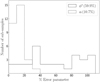 |
Fig. 12. Fractional error distribution of ϕ* and α after resampling the the OTELO field in 30 contiguous data cubes and estimate the corresponding luminosity function for testing the cosmic variance effects on these parameters. Values in the upper right corner correspond to the median values of these distributions. |
5.4. Star formation rate density
The LF may be integrated to obtain the total luminosity density. According to Schechter (1976), the integral is equal to:
where Γ is the gamma function.
After the integration, we obtain a value for the total luminosity density of  erg s−1 Mpc−3. This luminosity density can be translated to the SFRD via a Kennicutt (1998) equation:
![$$ \begin{aligned} \rho \,(M_\odot \,\mathrm{yr}^{-1}\,\mathrm{Mpc}^{-3})=&(1.4\pm 0.4)\times 10^{-41}\nonumber \\&\times {\mathcal{L} }{[{\text{ O}}{\small {{\text{II}}}}]3727}\,\mathrm{(erg\,s^{-1}\,Mpc^{-3})}, \end{aligned} $$](/articles/aa/full_html/2021/05/aa39880-20/aa39880-20-eq18.gif)
which is derived employing a Salpeter (1955) initial mass function (IMF). In order to convert this SFRD from the Salpeter IMF to the Kroupa (2001) IMF, we only need to multiply by a constant factor of 0.67 (Madau & Dickinson 2014). It has to be noted that the direct conversion of [O II]3727 luminosity to SFR may presents several problems, including metallicity and reddening dependencies (Khostovan et al. 2015). Nevertheless, it seems that the reddening is the main factor when deriving the SFR from [O II]3727 lines, as noted in Zhu et al. (2009) and Kewley et al. (2004).
We obtained a final result of  (erg s−1 Mpc−3). In Fig. 13 we plotted our derived value for the SFRD (red filled square) as a function of the redshift. In order to illustrate the SFRD evolution, we complemented the figure with results from the literature. All the data has been converted to a Kroupa IMF. The black dashed line is the fit done by Khostovan et al. (2015) following the parametrisation of Madau & Dickinson (2014):
![$$ \begin{aligned} \log \,(\rho )=a\frac{(1+z)^b}{1+[(1+z)/c]^d}, \end{aligned} $$](/articles/aa/full_html/2021/05/aa39880-20/aa39880-20-eq20.gif)
where a = 0.015, b = 2.26, c = 4.07, and d = 8.39.
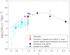 |
Fig. 13. SFRD evolution for several authors. The cyan circles are SFRD derived from [O II]3727, compiled by Khostovan et al. (2015) in the Table C.1 of their paper, and includes data from Ciardullo et al. (2013), Sobral et al. (2012), Bayliss et al. (2012), Ly et al. (2007), Zhu et al. (2009), Takahashi et al. (2007), Glazebrook et al. (2004), Teplitz et al. (2003), Gallego et al. (2002), Hicks et al. (2002), Hogg et al. (1998), and Hammer et al. (1997). We note that these points are not extinction-corrected, so they are a lower limit for the SFRD, as indicated by the cyan arrows. The filled black circles are data from Khostovan et al. (2015). The filled diamonds are data from Hayashi et al. (2020). The result of this work is represented by the open square. The red filled square represents the results of the SFRD from our LF but integrated with the ϕ* from Hayashi et al. (2013). The black dashed line is the [O II]3727 fit to the Khostovan et al. (2015) data, following the parametrisation of Madau & Dickinson (2014). |
It is clear from Fig. 13 that our result is below the curve, in a locus with the [O II]3727 data from the compilation. It must be noted that the SFRDs derived from Khostovan et al. (2015) compilation are not extinction-corrected, unlike our derived value for the SFRD. The data from Khostovan et al. (2015) and Hayashi et al. (2020) are located about ∼0.25 dex higher. This difference may be attributed to the low value of ϕ* due to the large uncertainties in the CV, as discussed in Sect. 5.3. Thereafter, this creates a lower value for the luminosity density when compared with their results, and, consequently, a lower value for the SFRD.
If we integrate our LF, but change the value derived for our ϕ* by the one obtained in Hayashi et al. (2013), the new derived SFRD (indicated in Fig. 13 by the filled red square) is now located over the line defined by Madau & Dickinson (2014) and has almost the same value as the SFRD derived by Khostovan et al. (2015) at the same redshift.
6. Summary and conclusions
We created a catalogue of 60 [O II]3727 emitters at ⟨z⟩ = 1.43, selected from data of the OTELO survey. We derived, from the pseudo-spectra, the redshifts, fluxes, and equivalent widths of all emitters. In Table A.1, we have catalogued all the emitters of the sample presented in this work.
Taking advantage of the ancillary data of the OTELO survey, we were able to fit galaxy templates to our emitters through the LePhare code. Thanks to this, we were able to derive extinctions for all the emitters and masses (or at least their upper bounds) for all the emitters. In total, 93% of the emitters were low-mass galaxies.
We were also able to obtain morphology parameters (Sérsic and concentration indices) for 44 of the emitters. The sérsic index derived for all of the emitters presented values compatible with disc galaxies. The majority of the [O II]3727 emitters are located in the bluer zone of the (u − r) versus morphology diagrams when compared with the rest of the galaxies of the OTELO survey. Also, all of them were classified as LT using the discriminant developed in de Diego et al. (2020). We detected four emitters with unusually high EW in [O II]3727 (Kong et al. 2002). One of them, id:8532, appears to be a low-mass disc galaxy.
The derived equivalent widths, having been binned and stacked, seem to follow the trends derived in Paulino-Afonso et al. (2020) and Khostovan et al. (2016) with the stellar mass. However, both Paulino-Afonso et al. (2020) (z ∼ 0.8) and Darvish et al. (2015) (z ∼ 0.5) present lower values for the equivalent width at larger masses when compared with Reddy & Steidel (2009), Khostovan et al. (2016) and our data (at z ∼ 1.5, z = 1.47, and z = 1.43 respectively). This may be due to the evolution of the equivalent width with the redshift, as suggested in Khostovan et al. (2016). Also, the lack of a clear correlation at lower masses for non-stacked sources detected in our data may be due the scarcity of emitters, as appears to be the case in Cava et al. (2015).
After we applied corrections for the completeness and the cosmic variance, among others, we obtained the LF for the [O II]3727 line, reaching almost 1 dex fainter than the works presented in literature. Nevertheless, our data present a lower value on log ϕ* when compared with other works. Because of the small cosmic volume sampled by OTELO when compared with modern NB surveys, the cosmic variance effects of the total uncertainties of LF data are quite large, and this propagates to the large variance obtained on this parameter. This effect can explain such differences with data provided in the literature.
On the other hand, the value α = −1.42 ± 0.06 obtained suggests a stepper slope on the faint end of the LF when compared with other authors (Drake et al. 2013 or Ly et al. 2007). This parameter is much less sensitive to the cosmic variance effects than the normalisation (ϕ*) of the LF. However, we obtain practically the same result as the one derived in Hayashi et al. (2013). As suggested by Sobral et al. (2011), this low value of α may indicate that we are (as well as Hayashi et al. 2013) sampling a low density field.
We have derived the SFRD by integrating the LF, employing the Kennicutt (1998) relationship and Kroupa (2001) IMF. We have found that the data from Khostovan et al. (2015) and from Hayashi et al. (2020) are at least ∼0.25 dex higher. This difference seems to come for our low value of ϕ* when compared with other results from literature (Ly et al. 2007; Drake et al. 2013 or Hayashi et al. 2013) and may be caused by the uncertainties presented in the normalisation of the LF due to CV effects.
The existence of a population of low-mass star-forming galaxies has been confirmed at z = 1.43. These galaxies present different characteristics when compared with the more massive populations at the same redshift that have been studied in several other works. This indicates that subsequent surveys with the same scope as demonstrated by OTELO are needed in order to complete a census of the galaxy populations at different epochs of the Universe.
Acknowledgments
This paper is dedicated to the memory of our affable colleague and friend Héctor Castañeda, who passed away on Nov. 19th, 2020. The authors thank the anonymous referee for her/his feedback and constructive suggestions, which have contributed to significantly improve the manuscript. BC wishes to thank Carlota Leal Álvarez for her support during the development of this paper. JAdD thanks the Instituto de Astrofísica de Canarias (IAC) for its support through the Programa de Excelencia Severo Ochoa and the Gobierno de Canarias for the Programa de Talento Tricontinental grant. This work was supported by the Spanish Ministry of Economy and Competitiveness (MINECO) under the grants AYA2013-46724-P, AYA2014-58861-C3-1-P, AYA2014-58861-C3-2-P, AYA2014-58861-C3-3-P, AYA2016-75808-R, AYA2016-75931-C2-1-P, AYA2016-75931-C2-2-P, and MDM-2017-0737 (Unidad de Excelencia María de Maeztu, CAB). This work was supported by the project Evolution of Galaxies, of reference AYA2017-88007-C3-1-P, within the “Programa estatal de fomento de la investigación científica y técnica de excelencia del Plan Estatal de Investigación Científica y Técnica y de Innovación (2013–2016)” of the “Agencia Estatal de Investigación del Ministerio de Ciencia, Innovación y Universidades”, and co-financed by the FEDER “Fondo Europeo de Desarrollo Regional”. This article is based on observations made with the Gran Telescopio Canarias (GTC) at Roque de los Muchachos Observatory of the Instituto de Astrofísica de Canarias on the island of La Palma. This study makes use of data from AEGIS, a multi-wavelength sky survey conducted with the Chandra, GALEX, Hubble, Keck, CFHT, MMT, Subaru, Palomar, Spitzer, VLA, and other telescopes, and is supported in part by the NSF, NASA, and the STFC. Based on observations obtained with MegaPrime/MegaCam, a joint project of the CFHT and CEA/IRFU, at the Canada–France–Hawaii Telescope (CFHT) which is operated by the National Research Council (NRC) of Canada, the Institut National des Science de l’Univers of the Centre National de la Recherche Scientifique (CNRS) of France, and the University of Hawaii. This work is based in part on data products produced at Terapix available at the Canadian Astronomy Data Centre as part of the Canada-France-Hawaii Telescope Legacy Survey, a collaborative project of NRC and CNRS. Based on observations obtained with WIRCam, a joint project of CFHT, Taiwan, Korea, Canada, France, at the Canada–France–Hawaii Telescope (CFHT), which is operated by the National Research Council (NRC) of Canada, the Institute National des Sciences de l’Univers of the Centre National de la Recherche Scientifique of France, and the University of Hawaii. This work is based in part on data products produced at TERAPIX, the WIRDS (WIRcam Deep Survey) consortium, and the Canadian Astronomy Data Centre. This research was supported by a grant from the Agence Nationale de la Recherche ANR-07-BLAN-0228.
References
- Anders, P., & Fritze-v Alvensleben, U. 2003, A&A, 401, 1063 [NASA ADS] [CrossRef] [EDP Sciences] [Google Scholar]
- Bayliss, K. D., McMahon, R. G., Venemans, B. P., Banerji, M., & Lewis, J. R. 2012, MNRAS, 426, 2178 [NASA ADS] [CrossRef] [Google Scholar]
- Bongiovanni, Á., Ramón-Pérez, M., Pérez García, A. M., et al. 2019, A&A, 631, A9 [NASA ADS] [CrossRef] [EDP Sciences] [Google Scholar]
- Bongiovanni, Á., Ramón-Pérez, M., Pérez García, A. M., et al. 2020, A&A, 635, A35 [NASA ADS] [CrossRef] [EDP Sciences] [Google Scholar]
- Bruzual, G., & Charlot, S. 2003, MNRAS, 344, 1000 [NASA ADS] [CrossRef] [Google Scholar]
- Calzetti, D., Armus, L., Bohlin, R. C., et al. 2000, ApJ, 533, 682 [NASA ADS] [CrossRef] [Google Scholar]
- Cava, A., Pérez-González, P. G., Eliche-Moral, M. C., et al. 2015, ApJ, 812, 155 [NASA ADS] [CrossRef] [Google Scholar]
- Cedrés, B., Beckman, J. E., Bongiovanni, Á., et al. 2013, ApJ, 765, L24 [NASA ADS] [CrossRef] [Google Scholar]
- Ciardullo, R., Gronwall, C., Adams, J. J., et al. 2013, ApJ, 769, 83 [NASA ADS] [CrossRef] [Google Scholar]
- Ciotti, L. 1991, A&A, 249, 99 [NASA ADS] [Google Scholar]
- Comparat, J., Richard, J., Kneib, J.-P., et al. 2015, A&A, 575, A40 [NASA ADS] [CrossRef] [EDP Sciences] [Google Scholar]
- Darvish, B., Mobasher, B., Sobral, D., et al. 2015, ApJ, 814, 84 [NASA ADS] [CrossRef] [Google Scholar]
- De Barros, S., Oesch, P. A., Labbé, I., et al. 2019, MNRAS, 489, 2355 [NASA ADS] [CrossRef] [Google Scholar]
- de Diego, J. A., Nadolny, J., Bongiovanni, Á., et al. 2020, A&A, 638, A134 [NASA ADS] [CrossRef] [EDP Sciences] [Google Scholar]
- Drake, A. B., Simpson, C., Collins, C. A., et al. 2013, MNRAS, 433, 796 [NASA ADS] [CrossRef] [Google Scholar]
- Gallego, J., García-Dabó, C. E., Zamorano, J., Aragón-Salamanca, A., & Rego, M. 2002, ApJ, 570, L1 [NASA ADS] [CrossRef] [Google Scholar]
- Garn, T., Sobral, D., Best, P. N., et al. 2010, MNRAS, 402, 2017 [NASA ADS] [CrossRef] [Google Scholar]
- Geach, J. E., Smail, I., Best, P. N., et al. 2008, MNRAS, 388, 1473 [NASA ADS] [CrossRef] [Google Scholar]
- Glazebrook, K., Tober, J., Thomson, S., Bland-Hawthorn, J., & Abraham, R. 2004, AJ, 128, 2652 [NASA ADS] [CrossRef] [Google Scholar]
- Hammer, F., Flores, H., Lilly, S. J., et al. 1997, ApJ, 481, 49 [CrossRef] [Google Scholar]
- Harish, S., Coughlin, A., Rhoads, J. E., et al. 2020, ApJ, 892, 30 [NASA ADS] [CrossRef] [Google Scholar]
- Hayashi, M., Sobral, D., Best, P. N., Smail, I., & Kodama, T. 2013, MNRAS, 430, 1042 [NASA ADS] [CrossRef] [Google Scholar]
- Hayashi, M., Ly, C., Shimasaku, K., et al. 2015, PASJ, 67, 80 [CrossRef] [Google Scholar]
- Hayashi, M., Shimakawa, R., Tanaka, M., et al. 2020, PASJ, 72, 86 [CrossRef] [Google Scholar]
- Herenz, E. C., Wisotzki, L., Saust, R., et al. 2019, A&A, 621, A107 [NASA ADS] [CrossRef] [EDP Sciences] [Google Scholar]
- Hicks, E. K. S., Malkan, M. A., Teplitz, H. I., McCarthy, P. J., & Yan, L. 2002, ApJ, 581, 205 [NASA ADS] [CrossRef] [Google Scholar]
- Hogg, D. W., Cohen, J. G., Blandford, R., & Pahre, M. A. 1998, ApJ, 504, 622 [NASA ADS] [CrossRef] [Google Scholar]
- Huang, X., Zheng, W., Wang, J., et al. 2015, ApJ, 801, 12 [NASA ADS] [CrossRef] [Google Scholar]
- Ibar, E., Sobral, D., Best, P. N., et al. 2013, MNRAS, 434, 3218 [NASA ADS] [CrossRef] [Google Scholar]
- Ilbert, O., Arnouts, S., McCracken, H. J., et al. 2006, A&A, 457, 841 [NASA ADS] [CrossRef] [EDP Sciences] [Google Scholar]
- Kauffmann, G., Heckman, T. M., White, S. D. M., et al. 2003, MNRAS, 341, 54 [Google Scholar]
- Kennicutt, R. C., Jr. 1992, ApJ, 388, 310 [NASA ADS] [CrossRef] [Google Scholar]
- Kennicutt, R. C., Jr. 1998, ARA&A, 36, 189 [Google Scholar]
- Kewley, L. J., Geller, M. J., & Jansen, R. A. 2004, AJ, 127, 2002 [NASA ADS] [CrossRef] [Google Scholar]
- Khostovan, A. A., Sobral, D., Mobasher, B., et al. 2015, MNRAS, 452, 3948 [NASA ADS] [CrossRef] [Google Scholar]
- Khostovan, A. A., Sobral, D., Mobasher, B., et al. 2016, MNRAS, 463, 2363 [NASA ADS] [CrossRef] [Google Scholar]
- Khostovan, A. A., Malhotra, S., Rhoads, J. E., et al. 2020, MNRAS, 493, 3966 [NASA ADS] [CrossRef] [Google Scholar]
- Kinney, A. L., Calzetti, D., Bohlin, R. C., et al. 1996, ApJ, 467, 38 [NASA ADS] [CrossRef] [Google Scholar]
- Kong, X., Cheng, F. Z., Weiss, A., & Charlot, S. 2002, A&A, 396, 503 [NASA ADS] [CrossRef] [EDP Sciences] [Google Scholar]
- Kroupa, P. 2001, MNRAS, 322, 231 [NASA ADS] [CrossRef] [Google Scholar]
- Lamareille, F., Contini, T., Le Borgne, J. F., et al. 2006, A&A, 448, 893 [NASA ADS] [CrossRef] [EDP Sciences] [Google Scholar]
- Lilly, S. J., Tresse, L., Hammer, F., Crampton, D., & Le Fevre, O. 1995, ApJ, 455, 108 [NASA ADS] [CrossRef] [Google Scholar]
- López-Sanjuan, C., Le Fèvre, O., Ilbert, O., et al. 2012, A&A, 548, A7 [NASA ADS] [CrossRef] [EDP Sciences] [Google Scholar]
- Ly, C., Malkan, M. A., Kashikawa, N., et al. 2007, ApJ, 657, 738 [NASA ADS] [CrossRef] [Google Scholar]
- Madau, P., & Dickinson, M. 2014, ARA&A, 52, 415 [NASA ADS] [CrossRef] [Google Scholar]
- Moster, B. P., Somerville, R. S., Newman, J. A., & Rix, H.-W. 2011, ApJ, 731, 113 [Google Scholar]
- Nadolny, J., Lara-López, M. A., Cerviño, M., et al. 2020, A&A, 636, A84 [NASA ADS] [CrossRef] [EDP Sciences] [Google Scholar]
- Nadolny, J., Bongiovanni, Á., Cepa, J., et al. 2021, A&A, 647, A89 [NASA ADS] [CrossRef] [EDP Sciences] [Google Scholar]
- Navarro Martínez, R., Pérez García, A. M., Pérez-Martínez, R., et al. 2020, Contributions to the XIV.0 Scientific Meeting (virtual) of the Spanish Astronomical Society, 66 [Google Scholar]
- Ouchi, M., Shimasaku, K., Akiyama, M., et al. 2008, ApJS, 176, 301 [NASA ADS] [CrossRef] [Google Scholar]
- Park, K., Di Matteo, T., Ho, S., et al. 2015, MNRAS, 454, 269 [Google Scholar]
- Paulino-Afonso, A., Sobral, D., Buitrago, F., & Afonso, J. 2017, MNRAS, 465, 2717 [NASA ADS] [CrossRef] [Google Scholar]
- Paulino-Afonso, A., Sobral, D., Darvish, B., et al. 2020, A&A, 633, A70 [NASA ADS] [CrossRef] [EDP Sciences] [Google Scholar]
- Ramón-Pérez, M., Bongiovanni, Á., Pérez García, A. M., et al. 2019, A&A, 631, A10 [NASA ADS] [CrossRef] [EDP Sciences] [Google Scholar]
- Reddy, N. A., & Steidel, C. C. 2009, ApJ, 692, 778 [NASA ADS] [CrossRef] [Google Scholar]
- Reddy, N. A., Shapley, A. E., Sanders, R. L., et al. 2018, ApJ, 869, 92 [NASA ADS] [CrossRef] [Google Scholar]
- Salpeter, E. E. 1955, ApJ, 121, 161 [Google Scholar]
- Schechter, P. 1976, ApJ, 203, 297 [Google Scholar]
- Sersic, J. L. 1968, Atlas de Galaxias Australes (Cordoba, Argentina: Observatorio Astronomico) [Google Scholar]
- Smit, R., Bouwens, R. J., Franx, M., et al. 2012, ApJ, 756, 14 [NASA ADS] [CrossRef] [Google Scholar]
- Sobral, D., Best, P. N., Smail, I., et al. 2011, MNRAS, 411, 675 [NASA ADS] [CrossRef] [Google Scholar]
- Sobral, D., Best, P. N., Matsuda, Y., et al. 2012, MNRAS, 420, 1926 [NASA ADS] [CrossRef] [Google Scholar]
- Sobral, D., Smail, I., Best, P. N., et al. 2013, MNRAS, 428, 1128 [NASA ADS] [CrossRef] [Google Scholar]
- Sobral, D., Matthee, J., Best, P. N., et al. 2015, MNRAS, 451, 2303 [NASA ADS] [CrossRef] [Google Scholar]
- Sobral, D., Santos, S., Matthee, J., et al. 2018, MNRAS, 476, 4725 [NASA ADS] [CrossRef] [Google Scholar]
- Somerville, R. S., Lee, K., Ferguson, H. C., et al. 2004, ApJ, 600, L171 [NASA ADS] [CrossRef] [Google Scholar]
- Strateva, I., Ivezić, Ž., Knapp, G. R., et al. 2001, AJ, 122, 1861 [CrossRef] [Google Scholar]
- Stroe, A., & Sobral, D. 2015, MNRAS, 453, 242 [NASA ADS] [CrossRef] [Google Scholar]
- Takahashi, M. I., Shioya, Y., Taniguchi, Y., et al. 2007, ApJS, 172, 456 [NASA ADS] [CrossRef] [Google Scholar]
- Teplitz, H. I., Collins, N. R., Gardner, J. P., Hill, R. S., & Rhodes, J. 2003, ApJ, 589, 704 [NASA ADS] [CrossRef] [Google Scholar]
- Thomas, D., Steele, O., Maraston, C., et al. 2013, MNRAS, 431, 1383 [NASA ADS] [CrossRef] [Google Scholar]
- Vika, M., Vulcani, B., Bamford, S. P., Häußler, B., & Rojas, A. L. 2015, A&A, 577, A97 [NASA ADS] [CrossRef] [EDP Sciences] [Google Scholar]
- Villaverde, M., Cerviño, M., & Luridiana, V. 2010, A&A, 517, A93 [NASA ADS] [CrossRef] [EDP Sciences] [Google Scholar]
- Zhu, G., Moustakas, J., & Blanton, M. R. 2009, ApJ, 701, 86 [NASA ADS] [CrossRef] [Google Scholar]
Appendix A: Catalogue and pseudo-spectra of the [O II]3727 emitters
In Table A.1, we summarise the main properties of our emitters. The distribution of columns is as follows: the first column is the OTELO identification number, the second and third columns are the coordinates of the sources in degrees, the fourth column is the redshift derived from the deconvolved model (zOTELO), the fifth column is the extinction in mag, the sixth column is the extinction corrected flux in units of 10−17 erg cm−2 s−1, the seventh column is the [O II]3727 equivalent width in Å, and the last column is the derived stellar mass.
Selected emitters.
In Fig. A.1, we represent, for all the emitters, the pseudo-spectrum flux in erg cm−2 s−1 Å−1, (black dots and black lines) and the deconvolved model (red line and same units), as a function of the wavelength in Å.
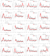 |
Fig. A.1. Pseudo-spectra of the selected emitters. Black dots represent the measured pseudo-spectra, the red line is the best fitted deconvolved spectra. |
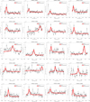 |
Fig. A.1. continued. |
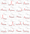 |
Fig. A.1. continued. |
All Tables
All Figures
|
Fig. 1. Pseudo-spectra and deconvolved spectra for the id:1494 emitter. We note the noisy aspect of the pseudo-spectra. However, in these circumstances, the model is capable of obtaining a good measure of the [O II]3727 lines. |
| In the text | |
|
Fig. 2. Pseudo-spectra and deconvolved spectra for the id:8532 emitter. The signal-to-noise ratio is better than in Fig. 1. |
| In the text | |
|
Fig. 3. Histogram of the value of A[O II]3727 for all the emitters in the catalogue. |
| In the text | |
|
Fig. 4. Histogram of the line flux (extinction corrected) observed for all the selected emitters. |
| In the text | |
|
Fig. 5. Observed (u − r) colour versus morphological parameters for all the sources of OTELO. From left to right: logarithm of the Sérsic index in the filter F814W (I), concentration index for the I filter too, and the logarithm of the wavelength-dependent ratio of the Sérsic indices for I and V (F606W). Triangles and solid lines in grey (histograms) represent LT, squares and dashed lines in black (histograms) represent ET galaxies. Red circles represent the [O II]3727 emitters from our sample with HST/ACS ancillary data. Top histograms corresponds to the respective value, as indicated in x-axis label, while right-hand histogram show (u − r) distribution. All histograms represents density distributions. Horizontal dot-dashed line in black shows (u − r) = 2.5. Red dashed line shows the results from de Diego et al. (2020). Dashed lines in magenta represent limits from Vika et al. (2015): horizontal cut in (u − r) = 2.3, while vertical dashed-lines in magenta represent log(nI) = 0.4 and |
| In the text | |
|
Fig. 6. Histogram of the derived stellar mass (in solar masses) for the emitters. The dashed line marks the position of the median value at log (M*/M⊙) = 8.87 and the point-dashed lines mark ±1σ over the median value. |
| In the text | |
|
Fig. 7. Histogram of the line equivalent width for all the selected [O II]3727 emitters in OTELO. The dashed line marks the position of the median value, and the point dashed lines mark ±1σ over the median value. |
| In the text | |
|
Fig. 8. Thumbnails in the OTELO composite filter (obtained adding all the slices of the scan) for the sources with high equivalent width. The red arrow indicates the location of the source. Each thumbnail has 8 × 8 arcsec size. From left to right: id:3077, id:3345, id:6445, and id:8532. |
| In the text | |
|
Fig. 9. Relationship between the [O II]3727 equivalent width and the derived stellar mass for our emitters (cyan open circles). The black diamonds are the median of our emitters for bins 0.5 dex in log(M*/M⊙), and the data from Paulino-Afonso et al. (2020) (red closed squares), Darvish et al. (2015) (filled purple stars for filament galaxies and green triangles for field galaxies), and Reddy et al. (2018) (grey diamonds). The black dashed line represents the best fit for all the binned data and the cyan point-dashed line represent the best fit for the only the binned data of the emitters detected in this work. The pink band represents the power law fit with uncertainties from Khostovan et al. (2016) for [O II]3727 emitters at z = 1.47. |
| In the text | |
|
Fig. 10. Mean of the detection probability of the [O II]3727 emitters at ⟨z⟩∼1.43. As described in Bongiovanni et al. (2020), the inset shows the detection probability distribution obtained from the simulations. The curve represents the least-square weighted fit of the sigmoid function. The bars indicated the mean standard error. |
| In the text | |
|
Fig. 11. Luminosity function for the [O II]3727 emitters at z ∼ 1.43 (black circles), with extinction and completeness corrected. The error bars correspond to the total uncertainties given in Table 4, and obtained as described in the text. The open circle marks the lowest luminosity bin and was not employed in the fitting. The black line is the best error-weighted fit of Schechter (1976) function. The green, blue, and orange lines are the LFs from Drake et al. (2013), Ly et al. (2007), and Hayashi et al. (2013) respectively. The shaded areas represent the propagation of 1σ uncertainties of the tabulated LF after 104 Monte Carlo realisations. For the OTELO data fitting, this propagation includes the standard deviation of the mean L* value. In each case, the solid line extend over the sampled luminosity range (see the right side columns in Table 4) and the dashed line is the extrapolation of the corresponding best fit. |
| In the text | |
|
Fig. 12. Fractional error distribution of ϕ* and α after resampling the the OTELO field in 30 contiguous data cubes and estimate the corresponding luminosity function for testing the cosmic variance effects on these parameters. Values in the upper right corner correspond to the median values of these distributions. |
| In the text | |
|
Fig. 13. SFRD evolution for several authors. The cyan circles are SFRD derived from [O II]3727, compiled by Khostovan et al. (2015) in the Table C.1 of their paper, and includes data from Ciardullo et al. (2013), Sobral et al. (2012), Bayliss et al. (2012), Ly et al. (2007), Zhu et al. (2009), Takahashi et al. (2007), Glazebrook et al. (2004), Teplitz et al. (2003), Gallego et al. (2002), Hicks et al. (2002), Hogg et al. (1998), and Hammer et al. (1997). We note that these points are not extinction-corrected, so they are a lower limit for the SFRD, as indicated by the cyan arrows. The filled black circles are data from Khostovan et al. (2015). The filled diamonds are data from Hayashi et al. (2020). The result of this work is represented by the open square. The red filled square represents the results of the SFRD from our LF but integrated with the ϕ* from Hayashi et al. (2013). The black dashed line is the [O II]3727 fit to the Khostovan et al. (2015) data, following the parametrisation of Madau & Dickinson (2014). |
| In the text | |
|
Fig. A.1. Pseudo-spectra of the selected emitters. Black dots represent the measured pseudo-spectra, the red line is the best fitted deconvolved spectra. |
| In the text | |
|
Fig. A.1. continued. |
| In the text | |
|
Fig. A.1. continued. |
| In the text | |
Current usage metrics show cumulative count of Article Views (full-text article views including HTML views, PDF and ePub downloads, according to the available data) and Abstracts Views on Vision4Press platform.
Data correspond to usage on the plateform after 2015. The current usage metrics is available 48-96 hours after online publication and is updated daily on week days.
Initial download of the metrics may take a while.