| Issue |
A&A
Volume 649, May 2021
|
|
|---|---|---|
| Article Number | A104 | |
| Number of page(s) | 27 | |
| Section | Stellar structure and evolution | |
| DOI | https://doi.org/10.1051/0004-6361/202039572 | |
| Published online | 21 May 2021 | |
Long-term X-ray spectral evolution of ultraluminous X-ray sources: implications on the accretion flow geometry and the nature of the accretor⋆
Institut de Recherche en Astrophysique et Planétologie, Université de Toulouse, UPS/CNRS/CNES, 9 Avenue du Colonel Roche, BP44346, 31028 Toulouse Cedex 4, France
e-mail: This email address is being protected from spambots. You need JavaScript enabled to view it.
Received:
1
October
2020
Accepted:
20
February
2021
Abstract
Context. The discovery of pulsations in several ultraluminous X-ray sources (ULXs) has demonstrated that a fraction of them are powered by super-Eddington accretion onto neutron stars (NSs). This has raised questions regarding the NS to black hole (BH) ratio within the ULX population and the physical mechanism that allows ULXs to reach luminosities well in excess of their Eddington luminosity. Is this latter the presence of strong magnetic fields or rather the presence of strong outflows that collimate the emission towards the observer?
Aims. In order to distinguish between these scenarios, namely, supercritically accreting BHs, weakly magnetised NSs, or strongly magnetised NSs, we study the long-term X-ray spectral evolution of a sample of 17 ULXs with good long-term coverage, 6 of which are known to host NSs. At the same time, this study serves as a baseline to identify potential new NS-ULX candidates.
Methods. We combine archival data from Chandra, XMM-Newton, and NuSTAR observatories in order to sample a wide range of spectral states for each source. We track the evolution of each source in a hardness–luminosity diagram in order to identify spectral changes, and show that these can be used to constrain the accretion flow geometry, and in some cases the nature of the accretor.
Results. We find NS-ULXs to be among the hardest sources in our sample with highly variable high-energy emission. On this basis, we identify M 81 X-6 as a strong NS-ULX candidate, whose variability is shown to be akin to that of NGC 1313 X-2. For most softer sources with an unknown accretor, we identify the presence of three markedly different spectral states, which we interpret by invoking changes in the mass-accretion rate and obscuration by the supercritical wind/funnel structure. Finally, we report on a lack of variability at high energies (≳10 keV) in NGC 1313 X-1 and Holmberg IX X-1, which we argue may offer a means to differentiate BH-ULXs from NS-ULXs.
Conclusions. We support a scenario in which the hardest sources in our sample might be powered by strongly magnetised NSs, meaning that the high-energy emission is dominated by the hard direct emission from the accretion column. Instead, softer sources may be explained by weakly magnetised NSs or BHs, in which the presence of outflows naturally explains their softer spectra through Compton down-scattering, their spectral transitions, and the dilution of the pulsed-emission should some of these sources contain NSs.
Key words: stars: neutron / stars: black holes / X-rays: binaries / accretion, accretion disks
Full Tables 1–3, and 7 are only available at the CDS via anonymous ftp to cdsarc.u-strasbg.fr (130.79.128.5) or via http://cdsarc.u-strasbg.fr/viz-bin/cat/J/A+A/649/A104
© A. Gúrpide et al. 2021
 Open Access article, published by EDP Sciences, under the terms of the Creative Commons Attribution License (https://creativecommons.org/licenses/by/4.0), which permits unrestricted use, distribution, and reproduction in any medium, provided the original work is properly cited.
1. Introduction
Ultraluminous X-ray sources (ULXs) are defined as extragalactic off-nuclear point-like sources with an X-ray luminosity in excess of ∼1039 erg s−1 (see Kaaret et al. 2017, for a review); although there is now evidence for a Galactic ULX (Wilson-Hodge et al. 2018). Their nature remains for the most part unknown, and given this empirical definition they likely constitute a heterogeneous population of objects. It was initially proposed that ULXs could be powered by accreting intermediate-mass black holes (IMBHs: ∼100−105 M⊙; see Mezcua 2017, for a review) in the sub-Eddington regime (Colbert & Mushotzky 1999; Matsumoto et al. 2001). The best ULX IMBH candidates may be those at the high-end of the high-mass X-ray binary (HMXB) luminosity distribution (e.g., Mineo et al. 2012), reaching LX ≥ 1041 erg s−1 in some cases. Some of these objects show transitions or temporal properties that seem to be consistent with the expectation of a scaled-up version of Galactic black hole binaries (GBHBs; e.g., Farrell et al. 2009; Godet et al. 2009; Pasham et al. 2014) and/or show evidence for cooler accretion disks (e.g., Feng & Kaaret 2010; Servillat et al. 2011; Godet et al. 2012; Lin et al. 2020) which suggest masses in the IMBH regime.
However, it was soon realised that the bulk of the ULX population (1039 < LX < 1041 erg s−1) did not comply with the canonical states seen in GBHBs (e.g., Stobbart et al. 2006; Gladstone et al. 2009; Grisé et al. 2010). It was therefore suggested that stellar-mass black holes (SMBHs) fed at super-Eddington mass-transfer rates could power these sources (Shakura & Sunyaev 1973; King & Pounds 2003; Poutanen et al. 2007), with geometrical beaming possibly further enhancing the observed luminosity (King et al. 2001). In this scenario, the intense radiation pressure blows off some of the excess gas in the form of a wind or outflow, which can become optically thick to the hard radiation emitted in the inner parts of the disk (Poutanen et al. 2007). The wind is expected to form a conic structure around the rotational axis of the compact object due to angular momentum conservation, producing highly anisotropic emission. It was then proposed that the short-term variability and the differences in spectral shape in a broad ULX sample could be understood in terms of different viewing angles and mass-accretion rates (Sutton et al. 2013; Middleton et al. 2015b) with those ULXs with LX ∼ 1039 erg s−1 showing a behaviour more consistent with SMBHs accreting close to or at their Eddington limit (e.g., Middleton et al. 2011). These studies were later extended to include ultraluminous supersoft sources (ULSs; Urquhart & Soria 2016), which are interpreted as sources in which the inclination of the system and/or the accretion rate are so high that the inner disk emission is completely reprocessed by the optically thick wind, with some sources possibly showing transitions between a ULX-like spectrum and a ULS state (Feng et al. 2016). Indeed, numerical simulations of super-Eddington accretion onto black holes (BHs) have shown extensively that the viewing angle has a strong impact on the observed spectrum (e.g., Ohsuga & Mineshige 2007; Sadowski et al. 2015; Ogawa et al. 2017). For this reason, it has been suggested that overall ULXs belong to a homogeneous class of objects, including SMBHs or weakly magnetised neutron stars (NSs), being fed at super-Eddington mass-transfer rates (King & Lasota 2016; King et al. 2017; Pinto et al. 2020a). Observational evidence supporting winds associated with super-Eddington accretion comes from high-resolution X-ray spectroscopy studies, which revealed absorption and emission features suggesting the presence of strong ionised winds colliding with the circumstellar medium (Pinto et al. 2016, 2017, 2020b).
However, while it was generally accepted that accreting SMBHs were the engines behind ULXs below 1041 erg s−1 (e.g., Poutanen et al. 2007; Gladstone et al. 2009; Pintore et al. 2014), the discovery of X-ray pulsations in one ULX (Bachetti et al. 2014) showed that NSs can also attain super-Eddington luminosities. Motivated by the discovery of (now) five more pulsating ULXs (PULXs; Fürst et al. 2016; Israel et al. 2017a,b; Carpano et al. 2018; Sathyaprakash et al. 2019; Rodríguez-Castillo et al. 2020) and the possible confirmation of another NS-ULX through the identification of a cyclotron line (Brightman et al. 2018), several authors have highlighted the remarkable X-ray spectral similarity of the ULX sample with those with detected pulsations (Pintore et al. 2017; Koliopanos et al. 2017; Walton et al. 2018a), suggesting that NS-ULX may dominate the ULX population. Yet, there is still some debate over the driving mechanism responsible for their extreme luminosities.
Pintore et al. (2017) suggested that the accretion column could be responsible for the hard emission in ULXs, as their X-ray emission could be described with a model commonly used to fit Galactic X-ray pulsars. Instead, based on the theoretical calculations carried out by Mushtukov et al. (2017), Koliopanos et al. (2017) argued that the ULX spectra are consistent with accreting highly magnetised NSs (B > 1012 G), as the 0.3−10 keV band can be described by two thermal components. In this scenario, the soft thermal component arises from a truncated accretion disk at the magnetospheric radius (Ghosh & Lamb 1978) while the hard emission is produced in an optically thick envelope as the accreting material is forced to follow the magnetic field lines, creating a closed envelope around the NS. The rotation of the envelope, which is due to the coupling with the NS through the magnetic field lines, and its latitudinal temperature gradient could explain the sinusoidal profiles seen in PULXs (e.g., Fürst et al. 2018), provided that the NS rotational axis is misaligned with the magnetic field axis. Alternatively, Walton et al. (2018a), following the arguments from King & Lasota (2016) and King et al. (2017), showed that the interplay between the mass-accretion rate and magnetic field strength could explain the lack or presence of pulsations in ULXs, suggesting that ULXs might instead be powered by weakly magnetised NSs. This in turn may explain the different spectral shape of those ULXs for which broadband spectroscopy data are available compared to the PULXs.
However, the long-term evolution of PULXs is marked by variability of two orders of magnitude or more in flux (Israel et al. 2017a,b) while other ULXs show variations of a factor of five or less on timescales of years (Grisé et al. 2013; Luangtip et al. 2016; Pinto et al. 2020b) with PULXs also being somewhat harder than the rest of the population (Pintore et al. 2017). Whether these represent differences in the nature of the accretor or are due to a disfavourable viewing angle (e.g., King & Lasota 2020) is still not fully understood (e.g., Walton et al. 2018a). If beaming is a natural consequence of super-Eddington mass transfer (King 2009), theoretical studies show that the fraction of observed BH-ULXs could be higher than NS-ULXs (Middleton & King 2017). Similarly, binary population synthesis studies suggest that BH-ULXs could even dominate the observed ULX population (Wiktorowicz et al. 2019), as NSs need stronger beaming factors to reach LX > 1039 erg s−1. However, evidence for supercritically accreting SMBHs remains elusive. The best observational evidence for such BH-ULX systems might be M 101 ULX-1, which was estimated to host a ∼20 M⊙ BH, although its dynamical mass determination was challenged by Laycock et al. (2015). Constraining the BH-to-NS ratio in ULXs can lead to important clues about the formation path leading to such systems and their connection with HMXBs (e.g., Mineo et al. 2012) and the formation of BH-BH and BH-NS systems.
Therefore, while the spectral resemblance of the ULX population is undeniable, tracing their long-term evolution could be key to understanding the geometry of the accretion flow and discriminating between super-Eddington accretion models and the nature of the accretor. To this end, we present a comprehensive study of the long-term spectral evolution of a representative sample of 17 ULXs (including 6 NS-ULXs) in the 1039 < LX < 1041 erg s−1 range in an effort to gain insight into the accretion flow geometry as well as the nature of the accretor. More specifically, we focus on studying the spectral evolution of each source in an attempt to assess which scenario best describes the variability observed: super-Eddington accretion onto a highly magnetised NS, a weakly magnetised NS, or a BH. This in turn provides clues about the nature of the accretor, and by comparing its evolution with the known PULXs, we can identify potential strong NS-ULX candidates. To do so, we build a phenomenological model taking into account the new information obtained on the ULX broadband emission with NuSTAR (Bachetti et al. 2014; Walton et al. 2015, 2020; Mukherjee et al. 2015) and track their spectral changes in a hardness–luminosity diagram (HLD).
We describe the sample of sources selected for this work and the data reduction in Sect. 2. In Sect. 3 we describe the data analysis and results. We discuss our results in Sect. 4 and present our conclusions in Sect. 5.
2. Sample selection and data reduction
2.1. Sample selection
In order to have a representative sample of the possible range of spectral variability of each source, we searched the literature for sources that have been observed on at least five occasions, well-spaced in time, by either XMM-Newton (Jansen et al. 2001) or Chandra (Weisskopf et al. 2000). We further required that they have either: high-quality XMM-Newton data (with ≳10 000 total counts in pn) or simultaneous broadband coverage with NuSTAR (Harrison et al. 2013) in at least one epoch. We were less stringent with the data constraints on the PULXs, because they are the only sources for which the nature of the accretor is known and thus they will be crucial for our study. We discarded M 82 X–2 from the current PULXs sample (NGC 7793 P13, NGC 5907 ULX1, NGC 300 ULX1, M 51 ULX–7, NGC 1313 X–2 and M 82 X–2), as this source is only resolved by Chandra and its spectra are frequently affected by pile-up. Its emission is also often contaminated with nearby sources and diffuse emission of unknown origin (Brightman et al. 2016), precluding a clean detailed spectral analysis of the source. Another source of interest is M 51 ULX–8, which was identified as harbouring an accreting NS through the detection of a cyclotron resonance feature (Brightman et al. 2018), although no pulsations have been reported to date. We therefore included this source in our sample to further investigate its spectral properties with respect to the PULXs.
For those ULXs for which the accretor is unknown, we included at least two sources from each of the different spectral regimes proposed by Sutton et al. (2013) in order to have a representative characterisation of the ULX population. We also made sure to include those sources showing evidence for super-Eddington outflows with 3σ detections (Pinto et al. 2016, 2017). Thus, we also included NGC 55 ULX1, even if it does not meet our criterion of having more than three epochs. The final sample selected for this study is presented in Table 1.
Sample of sources selected for this study with their respective distance, Galactic absorption (Kalberla et al. 2005; HI4PI Collaboration 2016), and log of observations considered.
Finally, we note that the luminosities reported for NGC 5907 ULX1 in this work are subject to an additional source of uncertainty, as there is a large discrepancy in the distance measurements to the host galaxy. The distance measurements range from ∼17 (Tully et al. 2016) to ∼12.9 Mpc (Crook et al. 2007) which can boost the inferred luminosity by a factor of ∼1.7. Here we adopted the most recent estimate of 17.06 by Tully et al. (2016).
2.2. Data reduction
XMM-Newton data reduction was carried out using SAS version 17.0.0. We produced calibrated event files from EPIC-pn (Strüder et al. 2001) and MOS (Turner et al. 2001) cameras with the latest calibration files as of March 2018 using the tasks epproc and emproc (version 2.24.1), respectively. We selected events from patterns 0 to 4 for pn and patterns ≤12 for the MOS cameras. The standard filters were used to remove pixels flagged as bad and those close to the CCD gaps. We created high-energy (10−12 keV) light curves from single pattern events from the full field of view to assess the presence of high-background particle flaring periods that could contaminate our spectra. We filtered these periods by removing times where the count rate was above a certain threshold by visually inspecting the light curves. These thresholds varied for each observation, and ranged from ∼0.3 cts s−1 to 1.2 cts s−1 and from ∼0.2 cts s−1 to 0.5 cts s−1 for the pn and MOS respectively.
Generally, we extracted source events from circular regions with a radius of 40″ and 30″ for pn and MOS respectively owing to their different angular resolution, rejecting observations in which the source fell on a chip gap. We reduced the source regions to avoid contamination from nearby sources, chip-gaps, or in cases where the source was faint in order to increase the S/N, but always ensuring that at least 50% of the PSF was enclosed. We used elliptical regions in cases where the source was placed at large off-axis angles, resulting in a distorted PSF. This was the case, for example, for the pn observations 0657801601 and 0657802001 of Holmberg IX X-1, observations 0112521001, 0112521101, 0657801801, 0657802001, 0657802201, 0693850801, 0693850901, 0693851001, and 0693851101 of M 81 X-6, and observation 0656580601 of Circinus ULX 5. The background region was selected from a larger circular source-free region and on the same chip as the source when possible. For the pn, we also tried to select the background region from the same distance to the readout node as for the source region. Finally, for M 51 ULX-7, we used regions of ∼20″ and ∼25″ for pn and MOS detectors respectively, to reduce contamination from the diffuse emission in which the source is immersed (Rodríguez-Castillo et al. 2020). We discuss possible contamination by the diffuse emission and its treatment in Sect. 3.1.1.
We noted also that Holmberg IX X-1 and Holmberg II X-1 were bright enough on some occasions to cause pile-up in the XMM-Newton detectors. We assessed the importance of pile-up using the tool epatplot (version 1.22) when the source count rate was above the recommended values1. In order to mitigate its effects, we excised the inner core of the PSF using an annular extraction region. The inner excised radius was never below 10.25″ and 2.75″ for the pn and the MOS cameras respectively, to avoid introducing inaccuracies in the flux estimation, as recommended2.
We finally used the tasks rmfgen (version 2.8.1) and arfgen (version 1.98.3) to generate redistribution matrices and auxiliary response files, respectively. We regrouped our spectra to have a minimum of 20 counts per bin to allow the use of χ2 minimisation and also avoided oversampling the instrumental resolution by setting a minimum channel width of one-third of the FWHM energy resolution.
We reprocessed the Chandra data using the script chandra_repro with calibration files from CALDB 4.8.2. We used extraction regions given by the tool wavdetect to extract source events. Background regions were selected from roughly three-times-larger, circular, nearby source-free regions. The level of pile-up was assessed by inspecting the images created using the pileup_map3 tool. We rejected observations with a pile-up fraction ≳5%. We only considered observations that registered ≥1000 counts, as we found that below this threshold data were of too poor a quality to robustly discriminate between different models. All data were also rebinned to a minimum of 20 counts per bin.
NuSTAR data were processed using the NuSTAR Data Analysis Software version 1.8.0 with CALDB version 1.0.2. We extracted source and background spectra using nuproducts with the standard filters. Source events were selected from a circular region of ∼60″. The only exception was NGC 1313 X-1, for which we followed Walton et al. (2016a) and chose a region of 40−50″ to reduce contamination from a nearby source (see Bachetti et al. 2013). Background regions were selected from larger circular source-free regions and on the same chip as the source but as far away as possible to avoid contamination from the source itself. We regrouped the NuSTAR spectra to 40 counts per bin, owing to the lower energy resolution compared to the EPIC cameras. For this work, we only considered NuSTAR observations for which simultaneous soft X-ray coverage with XMM-Newton was available. A summary of all observations considered can be found in Table 1.
3. Data analysis and results
We used the X-ray spectral fitting package XSPEC (Arnaud 1996) version 12.10.1f for spectral fitting and quote uncertainties on spectral parameters at the 90% confidence level for a single parameter of interest, unless stated otherwise. All fluxes were estimated using the pseudo-model cflux in XSPEC.
In general, we fitted EPIC data and the ACIS data in the 0.3−10 keV range. For the sources with the highest absorption columns (NGC 5907 ULX1, IC 342 X-1 and Circinus ULX5), we inspected the epatplot to choose the most suitable energy range to perform spectral fitting on the EPIC data. For IC 342 X-1 and Circinus ULX5, we noticed strong deviations from the observed pattern distributions with respect to the epatplot model below ∼0.4 keV. This is to be expected because the low-energy part of these absorbed spectra is likely dominated by the charge redistribution tail (and possibly noise). We therefore restricted the lower energy range to 0.4 keV for these two sources. For NuSTAR, we typically considered the 3−35 keV range, although to avoid including bins with negative number of counts in the χ2 minimisation we restricted the high-end of the energy range to those bins where the net number of counts was positive.
When simultaneously fitting spectra from different instruments from the same epoch, we attempted to compensate for calibration uncertainties by introducing a multiplicative cross-normalisation factor that was allowed to vary between the different instruments. This factor was frozen to unity for the pn (or the two MOS detectors if no pn data was available). We used the same factor for the MOS detectors as we found them to be generally in good agreement, while FPMA and FPMB each had their own separate constant, as recommended4. The agreement between the pn and the MOS cameras was usually within errors, with a few cases in M 81 X–6 where the disagreement reached 10% because of the highly elliptical distorted PSF caused by the off-axis position of the source on the detectors. The value of the cross-normalisation factor between EPIC data and NuSTAR detectors was typically in agreement within the errors, reaching a 5−20% disagreement in some cases, with the largest values found when the source was highly off-axis on the NuSTAR detectors.
Finally, we fitted together, that is, we assumed the same spectral model for two or more datasets if they were close in time (separated by a few days) and if after inspecting each observation separately we found no significant variation in flux and spectral parameters. This is also noted in Table 1 where we quote the different datasets that have been fitted together based on the above. Throughout this work, we use the word epoch to refer to all datasets that have been fitted together assuming the same model.
3.1. Spectral modelling
3.1.1. Choice of model
Our first aim was to characterise the long-term spectral evolution of our sample in a simple and coherent manner by studying variations of the spectral components (i.e. luminosity, radius, temperature, etc.). As the latest studies revealed that the 0.3−10 keV band can be modelled by two thermal components (e.g., Mukherjee et al. 2015; Koliopanos et al. 2017, 2019; Walton et al. 2020), which can reproduce the curvature seen at high-energies, we first considered a phenomenological model based on two multi-colour blackbody disks (diskbb in XSPEC; Mitsuda et al. 1984) to fit the data in this band, taking into account interstellar absorption by neutral hydrogen with two absorbing components tbabs in XSPEC. One was frozen at the Galactic value along the source line of sight (see Table 1), and the other one was left free to vary to take into account possible absorption from the host galaxy and the system itself. We adopted abundances given by Wilms et al. (2000) and cross-sections given by Verner et al. (1996) as recommended.
While other models have been commonly adopted to reproduce the hard emission (∼2 keV−10 keV) in ULXs, like Comptonisation of soft disk photons in a warm optically thick corona or a more phenomenological power law, we preferred the diskbb over these for various reasons. First of all, a warm optically thick corona up-scattering photons from the disk is merely a proxy to reproduce the curvature seen at high energies, as its physical interpretation is subject to several caveats (see Koliopanos et al. 2017, and references therein). Additionally, broadband spectroscopic studies have shown how this model fails to reproduce the spectral shape of ULXs (Walton et al. 2015; Mukherjee et al. 2015). Therefore, for the purpose of reproducing the spectral curvature in (at least) the XMM-Newton band, the diskbb has been shown to be equally valid with only two parameters. The power law (or a power law with a cutoff for the same matter) unphysically diverges towards low energies, thus taking up flux from the soft component and causing the absorption column to be overestimated.
Another advantage of the dual thermal component is that thanks to its simplicity, it can be used as a proxy to represent more complex models. For instance, in the context of super-Eddington accretion, the soft black body has been frequently associated with an outflow, while the hard one has been associated with emission from the inner parts of the accretion flow (e.g., Walton et al. 2014). Alternatively, Koliopanos et al. (2017) associated the soft component with an accretion disk truncated at the magnetospheric radius, and attributed the hard component to the emission from the magnetospheric envelope (Mushtukov et al. 2017). The diskbb also allows us to easily test theoretical predictions by studying the evolution of its temperature with its luminosity as we show in Sects. 3.4 and 3.5.
However, visual inspection of the fit residuals revealed strong residuals at high energies in the 0.3−10 keV band in some epochs, indicating that our phenomenological model is not able to reproduce the emission at high energies. We show this for two high-quality observations of Holmberg II X-1 and NGC 5408 X-1 in Fig. 1. This is perhaps not surprising, as broadband studies using NuSTAR data have revealed the presence of a faint hard power-law-like excess dominating above ∼10 keV (e.g., Mukherjee et al. 2015; Walton et al. 2015, 2017). We find that for those epochs for which we have broadband coverage with NuSTAR, this excess can be well modelled as Comptonisation of the hot thermal component as noted by previous studies. As the nature of this Comptonisation component is still poorly understood (Walton et al. 2017) and given the lack of broadband coverage for most of the observations considered here, we decided to use the simpl model (Steiner et al. 2009) to reproduce it, as this latter does not assume any geometry but simply scatters a fraction of photons (fscat) of the seed component towards high energies, emulating a power-law component with a certain Γ, with the advantage that it does not diverge towards low energies.
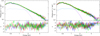 |
Fig. 1. Unfolded pn (blue), MOS1 (red), and MO2 (green) spectra fitted with an absorbed dual thermal component (tbabs⊗tbabs⊗ (diskbb + diskbb)) on (left) observation 0200470101 of Holmberg II X-1 ( |


In order to identify those epochs for which the simpl model component is required, we would ideally rely on Monte-Carlo simulations. However, given the large number of datasets considered here this is not feasible. Instead, to obtain an estimate as to when the data quality allows us to constrain this component, we performed an F-test between the dual-thermal model described above and the model tbabs⊗tbabs⊗ (diskbb + simpl⊗diskbb) and decided to include the simpl model only if the probability of rejecting (Prej) the simpler model was ∼3σ. We also included the simpl model for observations with Prej slightly below this value if we were able to constrain its parameters using near-in-time observations with Prej > 3σ (see below). Similarly, we excluded the simpl component in some cases with Prej > 3σ if its parameters are largely unconstrained. We are aware that this is not an appropriate use of the F-test, however the presence of this component was already shown to be significant by Walton et al. (2018a) and indeed we found that this component was required to fit the highest quality datasets. We are not claiming to confirm this component as present or not, but instead we used these values as a reference indicating when the data quality allows this component to be constrained. We present the result of this F-test in Table 7 where we also indicate for which observations we finally included this component.
For NGC 7793 P13 we found that this component is largely unconstrained even in the broadband datasets, resulting in no fit improvement when adding this component. The broadband datasets yield fits with  ∼ 1.1 with the dual-thermal model alone, which are statistically acceptable, and so we decided not to add this component.
Furthermore, as the simpl model is mostly responsible for the emission above ∼8 keV in our modelling, its parameters are not well constrained when Chandra or XMM-Newton data are considered alone, and only in long XMM-Newton exposures with > 40 000 counts in pn can we constrain both fscat and Γ simultaneously. We also found good consistency between the Γ-values in several epochs and that most sources are found recurrently at similar fluxes and hardness ratios (see Sect. 4). We therefore tied Γ across epochs where the source is found at similar flux and hardness ratio, while leaving fscat and the rest of the parameters free to vary. By doing so we were able to use the broadband information provided by NuSTAR to have some constraints on those epochs where this information is not available. For NGC 1313 X-1, after checking the consistency of Γ across epochs and bearing in mind that its variability above 10 keV has been shown to be small (Walton et al. 2020), we tied Γ for all observations where the simpl model is used. For NGC 5408 X-1 and NGC 6946 X-1, we also found very little variability at high-energies and therefore we again tied Γ across all observations where we added the simpl model. Finally, for NGC 1313 X-2, we also found that the same Γ-value can be tied for the four epochs for which we included the simpl model, although in this case the source shows a certain variability at high energies (see Sect. 3.3).
For M 81 X-6, M 51 ULX-7, M 51 ULX-8, and M 83 ULX1, given the lack of broadband coverage and that the dual-thermal model gave an acceptable fit to the data, we found no need to try to improve the fit by adding the simpl model and therefore we did not explore this option. As stated in Sect. 2, the XMM-Newton observations of M 51 ULX-7 might be contaminated by some diffuse emission. To quantify the possible contamination from this diffuse emission, we extracted two MOS1 and MOS2 spectra (from obs id 0824450901) from two circular (25″ in radius) regions located 34″ from the source in two different directions. We fitted both emission spectra with a powerlaw and a mekal model subject to Galactic absorption only. The spectral parameters of both spectra are consistent within errors with Γ = 2.9 and 2.8 ± 0.3, and plasma temperature = 0.28 ± 0.03 keV and 0.27
 keV for region 1 and 2 respectively. We therefore ruled out strong spatial variations and computed the luminosity of region 1. We find a total unabsorbed luminosity of (4.9
 ) × 1038 erg s−1 in the 0.3−10 keV band, with the soft band (0.3−1.5 keV) being approximately five times brighter than the hard band. We therefore estimate that the diffuse emission can make the source appear ∼25% softer in the XMM-Newton observations, given that M 51 ULX-7 has a typical luminosity of 4 × 1039 erg s−1. We therefore added this diffuse emission model as a fixed additive component to the M 51 ULX-7 continuum in all XMM-Newton observations and decided to discard obsids 0677980701, 0677980801, and 0830191401 when the source was at its lowest.
Finally, some sources show strong residuals at soft energies, which have been associated with unresolved emission and absorption lines produced in an outflow colliding with the circumstellar gas (Pinto et al. 2016, 2017, 2020b). In most cases, we ignored them, as we are interested in the continuum emission and this will not affect our results. There are two exceptions to this: for NGC 5408 X-1, including a Gaussian emission line at ∼1 keV leads to a Δχ2 improvement that ranges from ∼50 to 122 (for 3 extra degrees of freedom) depending on the observation. We therefore decided to also determine the parameters of this Gaussian in the joint fit of the high-quality datasets by tying together all its parameters. We obtain E = 0.947 ± 0.005 keV, σ = 78 ± 6 eV and normalisation = 2.7 × 10⁻⁵ photons cm−2 s−1. For NGC 5204 X-1, we also included a Gaussian emission line for the Chandra obsid 3933 following Roberts et al. (2006) as we again note similar strong residuals. In this case we obtain E = 0.97 ± 0.02 keV, σ = 56
 eV and normalisation = 2 ± 1 × 10⁻⁵ photons cm−2 s−1, consistent with the values reported by Roberts et al. (2006).
3.1.2. Treatment of the absorption column
There is still no consensus as to whether the local absorption column in ULXs is variable (e.g., Kajava & Poutanen 2009) or not (e.g., Miller et al. 2013). The main argument for variability of the absorption column in ULXs is the contribution from outflows (e.g., Kajava & Poutanen 2009; Middleton et al. 2015a), which could imprint stochastic variability in nH due to wind clumps crossing our line of sight (Takeuchi et al. 2013; Middleton et al. 2015b) depending on their column density and ionisation state. Alternatively, Middleton et al. (2015a) argued that some expelled gas could cool down far from the source and contribute to the neutral absorption column. If this is the case, it is then not clear over what timescale nH would react to instantaneous changes in the mass-accretion rate.
To make matters more complicated, Miller et al. (2009), studying absorption edges at high spectral resolution in X-rays, showed that the absorption column remains stable throughout spectral changes in a set of X-ray binaries, and that changes in the soft component must come from changes in the source spectrum and not from the absorption column itself.
In view of these complications, we attempted to study variations in nH by fitting all epochs individually for each source using the dual-thermal component over the 0.3−8 keV band, so as to use the same model for all epochs and avoid introducing artificial changes in nH due to the different energy ranges considered when using NuSTAR data. We find that in general, the values of the absorption column for a given source are consistent within 3σ errors over all epochs, which we show in Fig. 2 for four sources in our sample. Small discrepancies can be attributed to low data quality (e.g., short exposure Chandra observations and/or calibration uncertainties) rather than real physical-nH changes. For NGC 5408 X-1, when fitting the 0.3−8 keV band with the dual-thermal model we still see strong residuals at high energies, which may indicate that the dual-thermal model cannot adequately fit the 0.3−8 keV band. We therefore repeated the study of the nH variations replacing the hard diskbb with a power law with a high-energy cutoff (cutoffpl in XSPEC) to ensure that the lack of mismodelling of the high-energy emission does not affect the nH variations (or lack of) found before. With this model we again find all nH values consistent at the 3σ level.
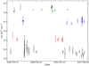 |
Fig. 2. Evolution of the local absorption column over time for NGC 5408 X-1 (green), NGC 7793 P13 (blue), Holmberg IX X-1 (red), and NGC 1313 X-2 (black) shifted by 0.2 × 1022 cm−2 for clarity. All spectra have been fitted with a model consisting of an absorbed dual diskbb model in the 0.3−8 keV band. Errors are shown at 3σ confidence level. Circles and squares correspond to XMM-Newton and Chandra data respectively. |
Conversely, we did find evidence for variability in the absorption column of NGC 1313 X-1 and NGC 55 ULX1 when following the same approach, where variations above the 3σ confidence level were seen (see the arrows in Fig. 3). However, given the phenomenological nature of our model, we cannot rule out the possibility that these discrepancies are due to a change in the underlying continuum, therefore changing the parameter degeneracies.
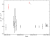 |
Fig. 3. As in Fig. 2 but for NGC 1313 X-1 (black) and NGC 55 ULX1 (red). Arrows indicate epochs where a 3σ significant change is seen with respect to some other epochs (see text for details). |
For the other sources not discussed here, we do not find such strong evidence for variability in the absorption column as for the sources discussed above, although in some cases this could be due to poorly constrained model parameters. Therefore, in view of the above considerations, we consider that the absorption column can be assumed to be constant for the most part, with the exception of epoch 2004-08-23 of NGC 1313 X-1 and epoch 2010-05-24 of NGC 55 ULX1. In these cases we allowed nH to vary together with the continuum parameters as this is preferred by the fit. We find Δχ2 improvements of ∼25 and 15 for NGC 1313 X-1 and NGC 55 ULX1 respectively when leaving nH free, compared to the case where nH is frozen to the average value (see following section). We discuss this in more detail in Sect. 4.4.
3.1.3. Spectral fitting approach
Ideally, we would jointly fit all datasets for each source, tying the nH and Γ across certain datasets as explained above. However, such a procedure would be computationally prohibitive. As the joint fit will mostly be driven by those datasets with higher data quality, in order to reduce the computational burden of this approach we decided to do our spectral fitting in two steps: we first jointly fitted those datasets with better statistics, tying together Γ across those epochs where the source is found at similar flux and hardness ratio and nH across all epochs, while leaving the remaining parameters free to vary. We typically consider three to eight datasets for each source, which includes those observations with the longest XMM-Newton exposures when the three EPIC cameras are operational, those for which simultaneous NuSTAR coverage is available and in some rare cases, the longest Chandra observations. We next fitted the remaining observations of lower data quality individually with nH and Γ frozen at the values found in the joint fit. The results of the joint and the subsequent individual fits are reported in Table 2.
Best-fit spectral fit parameters.
For Circinus ULX5, the joint-fit approach results in largely unconstrained parameters for the low-energy components at soft energies. This is likely due to a combination of the calibration uncertainties at low energies (see Sect. 3) and the high absorption column along the line of sight (nH Gal = 50.6 × 1020 cm−2; HI4PI Collaboration 2016). We therefore considered only epoch 2013-02-03 to constrain nH as it offers the best constrains on the broadband emission.
3.2. Hardness–luminosity diagram
As a first source classification and in order to highlight the differences and similarities between the sources in our sample, we started by building a HLD similar to that often used for X-ray binaries (Done & Gierliński 2003) and also for ULXs (e.g., Sutton et al. 2013). We did this by computing unabsorbed fluxes rather than counts because relying on count rates is not feasible given the different instruments employed for this work. Furthermore, fluxes have the advantage that they can be corrected for absorption column. To do this, we retrieved the total unabsorbed luminosity in the 0.3−10 keV band from the tbabs⊗tbabs⊗ (diskbb + simpl⊗diskbb or diskbb) depending on the epoch. The hardness ratio is computed as the ratio of unabsorbed fluxes in a soft band (0.3−1.5 keV) and a hard band (1.5−10 keV). This is motivated by the fact that the pulsating component in PULXs has been shown to dominate at high energies (e.g., Israel et al. 2017a; Walton et al. 2018b) and thus we may expect to highlight the differences between pulsating and non-pulsating sources, while the soft component in ULXs usually stops dominating above ∼1 keV.
Indeed, the results presented in Fig. 4 and Table 3 show clearly that PULXs are harder than the rest of the sample, with some interesting exceptions. In general, PULXs harden in the 0.3−10 keV band with luminosity with high levels of flux variability. We find that most of the population reaches a maximum luminosity of ∼2 × 1040 erg s−1, with just Holmberg IX X-1 and NGC 5907 ULX1 above this value. This is also highlighted in Fig. 5, where a drop in sources reaching a maximum luminosity ∼2 × 1040 erg s−1 is clearly seen.
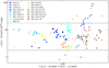 |
Fig. 4. Hardness–luminosity diagram for the ULX sample selected for this study. All fluxes and luminosities are unabsorbed. PULXs are shown in shades of orange and the epochs for which pulsations have been reported in the literature (Israel et al. 2017a; Fürst et al. 2018; Carpano et al. 2018; Vasilopoulos et al. 2018; Sathyaprakash et al. 2019; Rodríguez-Castillo et al. 2020) are highlighted by a black edge around the marker. The dashed black lines indicate respectively 10 and 100 times the Eddington limit for a NS (∼2 × 1038 erg s−1). |
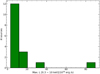 |
Fig. 5. Histogram of the maximum unabsorbed luminosity in the 0.3−10 keV band attained by each source considered in this work. A clear drop of sources with L ≥ 2 × 1040 erg s−1 is seen. |
Lastly, we note that as we have rejected observations below ∼1000 counts, transitions to the off states below ∼1039 erg s−1 like those seen for NGC 5907 ULX-1 (Israel et al. 2017a), NGC 7793 P13 (Israel et al. 2017b), or M 51 ULX-7 (Brightman et al. 2020) are not reflected in this diagram.
3.3. Spectral transitions
We also present the temporal evolution of each individual source in the HLD in Fig. 6, along with the unfolded spectra of some selected epochs. For this, we selected two to four clearly distinct spectral states based on the HLD in order to highlight the possible range of spectral variability of each source. When possible, we selected observations for which NuSTAR data are available so that the broadband variability can be observed. We caution that given the sparse monitoring offered by XMM-Newton and Chandra in some cases, care must be taken when looking at the source variations in the HLD. Arrows indicate the chronological order but in many cases we cannot guarantee that the source did not evolve differently between the epochs considered here.
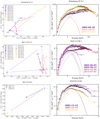 |
Fig. 6. Left: temporal tracks on the HLD. Filled coloured markers indicate fluxes obtained from XMM-Newton data, unfilled markers indicate fluxes obtained from joint XMM-Newton-NuSTAR data, and black-filled markers indicate fluxes obtained from Chandra data. The legend indicates the date of the epoch in each case. Right: unfolded spectra for selected epochs in which the source has experienced strong changes, following the same colour-code as for the left panels. Selected epochs are indicated in the legend. For the EPIC data, only pn is shown (circles) or MOS1 if pn is not available (as triangles up). In cases where we have used NuSTAR data, FPMA is shown, represented as squares and with the same colour as pn. Chandra data are shown with downward-pointing triangles. The soft and hard diskbb model components are shown with a dashed line and dotted line respectively, while the total model is shown with a solid line. For epochs where the simpl model has been used see Table 2. Data have been rebinned for clarity. |
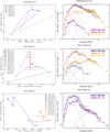 |
Fig. 6. continued. |
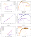 |
Fig. 6. continued. |
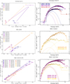 |
Fig. 6. continued. |
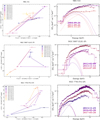 |
Fig. 6. continued. |
 |
Fig. 6. continued. |
3.4. Spectral evolution of the soft thermal component
Several authors have attempted to study the nature of the soft component in ULX spectra by investigating its evolution on the luminosity–temperature (L–T) plane (e.g., Kajava & Poutanen 2009; Miller et al. 2013). However, these studies have frequently yielded contradictory results and thus there is still no consensus on its true nature. We therefore investigated the correlation of the bolometric luminosity of the cool diskbb component with its temperature. We did this by retrieving unabsorbed luminosities of the diskbb component in the 0.01−100 keV5. All fluxes are reported in Table 3. We did not attempt to derive any correlation for NGC 55 ULX1 and NGC 300 ULX1 because of the limited number of observations available for these sources.
We next assessed whether L–T are correlated by running a Spearman correlation test6. The results are reported in Table 4. Five of our sources show a strong positive L–T correlation (Spearman correlation ≥0.5 and a p-value of ≲0.05). For these, we fitted a power law using the python routine odr7, which takes into account both errors on x and y variables (see Fig. 7 and Table 4 for the results). In order to investigate whether these correlations were driven by the degeneracy between Tsoft and its normalisation, we derived 99% χ2 confidence contours around the best-fit Tsoft and its normalisation for those sources showing a positive L–T correlation. Given the extensive computational time required by the steppar command in XSPEC, we did this only for some selected epochs, ensuring that at least one was from the joint fit. The results are shown in Fig. 8 for NGC 1313 X-1, Holmberg IX X-1, Holmberg II X-1, and NGC 5204 X-1, where we also overlaid the best-fit Tsoft and normalisation from all epochs. In all cases where a positive L–T correlation is observed, including IC 342 X-1, which we did not show for brevity, a strong degeneracy between the Tsoft and its normalisation is observed, highly correlated with the datapoints from the individual observations, indicating that the L–T correlations are simply due to a degeneracy between these two parameters.
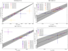 |
Fig. 7. Examples of sources showing a positive correlation between the soft diskbb component unabsorbed bolometric luminosity and its temperature. The black line shows the best-fit power law with grey shaded areas indicating the 90% confidence interval on the exponent. Symbols are coloured as per Fig. 6. The data have been fitted with the model tbabs⊗tbabs⊗ (diskbb + simpl⊗diskbb or tbabs⊗tbabs⊗ (diskbb + diskbb)) (see text for details). |
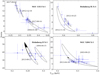 |
Fig. 8. 99% χ2 contours (solid black lines) between Tsoft and its normalisation for sources showing a positive L–T correlation. For each source, two to four different epochs are represented with the epoch indicated next to the contour. A clear anti-correlation is seen in all cases that closely follows the best-fit values from all the epochs (blue datapoints, 90% confidence level error bars), which indicates that the L–T positive correlation is due to the degeneracy between these two parameters. For the sake of readability, we have ignored epoch 2004-06-05 in the panel of NGC 1313 X-1 as it had a much higher normalisation (∼51) compared to the other observations. |
Results of the L–T correlation for the soft thermal component.
For M 81 X-6, while the correlation test could indicate a positive correlation, visual inspection of the data clearly reveals that there is no apparent trend (see Fig. 9). We recall that the Spearman’s test coefficient does not take into account errors on the parameters and hence these values need to be treated with caution. In fact, the fit with the power law yields a large error on the index α = 2.5 ± 2.0 (90% confidence level), while the normalisation is consistent with zero.
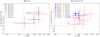 |
Fig. 9. As for Fig. 7 but for sources showing no correlation between the soft diskbb bolometric luminosity and its temperature. |
3.5. Spectral evolution of the hard thermal component
Similarly, we studied the hard thermal component evolution in the L–T plane. In cases where we employed the simpl model on this component, we retrieved the intrinsic flux of the hard diskbb using cflux as simpl⊗cflux⊗diskbb and freezing the normalisation of the diskbb. Derived fluxes are presented in Table 3 and the results from the L–T correlation are shown in Table 5.
Results of the L–T correlation for the hard thermal component.
Most of the sources show no clear correlation in the hard thermal component. The only exception is M 83 ULX1, which shows a strong positive correlation (Spearman correlation of 0.94 with a p-value = 0.005, see Fig. 10). We again computed χ2 contours around the best-fit temperature and normalisation for some selected epochs and overlaid the results from the spectral fitting on them as shown in Fig. 10. In this case, it seems that the degeneracy between these two parameters is not driving the existing correlation.
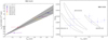 |
Fig. 10. Left: as for Fig. 7 but for M 83 ULX1 for the hard diskbb. Right: as for Fig. 8 but for the countours around the best-fit Thard and its normalisation for three selected epochs of M 83 ULX1. The degeneracy between these two parameters can be ruled out as the cause of the positive L–T correlation. |
While NGC 6946 X-1 might seem positively correlated based on the Spearman test alone, examination of the data clearly reveals that there is an overall lack of strong variation of the hard component in most observations (see Fig. 11). Furthermore, we note a certain bias in those observations for which we have not included the simpl model, as the temperature of the hard diskbb appears to be systematically higher, as the diskbb is pushed towards high energies because of the lack of an additional high-energy component.
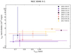 |
Fig. 11. Bolometric luminosity of the hard diskbb component as a function of its temperature for NGC 6946 X-1. Because of the uncertainties associated with the parameters, we do not consider these two quantities to be correlated (see text for details). Symbols as per Fig. 6. |
4. Discussion
We examined the long-term spectral evolution of a sample of sources containing known PULXs and ULXs for which the accretor is unknown, in order to gain insight into their nature and the accretion processes driving their extreme luminosities. While our spectral fitting approach is phenomenological, we attempted to understand the nature of the soft and the hard components by means of L–T correlations. The positive L–T correlations for the soft component found in Sect. 3.4 are broadly consistent with previous results reported by Miller et al. (2013), who studied a similar sample of sources and also assumed a constant absorption column, albeit using a different model based on an accretion disk whose photons are Compton-up scattered by an optically thick corona of hot (Te > 2 keV) electrons. Similar correlations were also reported for NGC 5204 X-1 and Holmberg II X-1 by Feng & Kaaret (2009) using an absorbed diskbb and a power law. These correlations have frequently been used to argue in favour of an accretion disk as the nature of the soft component in ULXs. However, our analysis reveals that these are driven by the existing degeneracy (see Fig. 8) between the temperature of the soft component and its normalisation and therefore these relationships cannot be used reliably to support this scenario. Indeed, it has been shown that depending on the assumption of the underlying model, the correlation can disappear entirely (see e.g., Luangtip et al. 2016; Walton et al. 2020; see also Gonçalves & Soria 2006 for a discussion on the weaknesses of associating the soft component with an accretion disk). Nevertheless, these correlations might be useful to identify sources evolving in a similar fashion.
Conversely, the positive L–T correlation found for the hard thermal component of M 83 ULX1 might have a physical origin, as we argue in Sect. 4.6, given that this correlation is not driven by the existing degeneracy between the parameters (see Fig. 10).
Similarly, Kajava & Poutanen (2009) used the found negative L–T correlation for the soft component to argue in favour of an outflow as the nature of the soft component. However, this result was likely artificially created by employing a power law for the high-energy emission while leaving the absorption column free to vary. We therefore suggest that the beaming formalism derived by King (2009) using the results from Kajava & Poutanen (2009), linking the mass-transfer rate (ṁ0) with the beaming factor (b) for super-Eddington accretion onto BHs or weakly magnetised NSs, should be revisited in view of these new results. Overall, our study suggests that given the limitation from using phenomenological models to describe the ULX continuum, the observed changes in the best-fit spectral parameters may not be the most appropriate way to build a physical picture for our sources. For this reason, most of our discussion will be based on the variability observed in terms of luminosity and hardness ratios (see Figs. 4 and 6).
Figures 4 and 5 show that most sources seem to have a maximum luminosity of roughly 2 × 1040 erg s−1. M 51 ULX-7 and M 82 X-2 (the other PULX not analysed in this work) also reach luminosities of a few × 1040 erg s−1 (Brightman et al. 2016, 2020). While the sample presented here is rather small in a statistical sense, it confers the advantage that we can take into account the long-term variability of each source; it is also free of contaminants and the absorption column has been carefully estimated. On this basis, our work seems to support larger sample studies (Swartz et al. 2011), where a possible cutoff at around 2 × 1040 erg s−1 was observed in the luminosity function of a sample of 107 ULX candidates. Mineo et al. (2012) showed that ULXs seem to extend the X-ray luminosity function of HMXBs up to a possible energy cutoff also at around 2 × 1040 erg s−1, supporting the idea that ULXs are an evolutionary stage of HMXBs. Thus, ULXs might be related to systems where the companion star expands and starts to fill its Roche Lobe as suggested by King & Lasota (2020). As NS accretors are more numerous among HMXBs (e.g., Casares et al. 2017), it is possible that a substantial fraction of ULXs with LX ∼ 1039−41 erg s−1 could host a NS. However, we stress that given the limited sample studied here, we may be running into small numbers when distinguishing a cutoff distribution from a power-law one (Walton et al. 2011).
A luminosity cutoff around 2 × 1040 erg s−1 would be consistent with the maximum accretion luminosity NSs can attain according to Mushtukov et al. (2015). These latter authors considered the accretion column model proposed by Basko & Sunyaev (1976) and the reduction of the electron scattering cross-section in the presence of high-magnetic fields that allows the Eddington limit to be overcome. Mushtukov et al. (2015) suggest that NSs could reach ∼1040 erg s−1 for a reasonable parameter space of magnetic fields and spin periods. Indeed, the hard component (the diskbb or the more complex simpl⊗diskbb when applicable) that we would associate with the accretion column (e.g., Walton et al. 2018c) reaches a maximum luminosity of ∼1040 erg s−1 in NGC 7793 P13, M 51 ULX-7, and NGC 1313 X-2. However, the fact that we find a PULX (NGC 5907 ULX1) also above the break is problematic. The hard component is a factor of about eight above this theoretical value. It is possible that by assuming isotropic emission in our luminosity calculations, we may be overestimating the luminosity of the accretion column. We discuss this in more detail in Sect. 4.1.
On the other hand, general relativistic radiation magnetohydrodynamic (GRRMHD) numerical simulations of super-Eddington accretion onto BHs also predict saturation of the maximum luminosity with the mass-accretion rate (Narayan et al. 2017), as the models of these latter authors start to become radiatively inefficient above ∼10 ṀEdd. Their simulations show that the observed luminosity saturates at 2 × 1040 erg s−1 for a 10 M⊙ BH viewed close to face-on, which might be supported by our observations.
The mass-transfer rate (ṁ0) in ULXs is generally accepted to be super-Eddington, even if the sustainability of such a process at such extremes over long timescales (sometimes over several decades) has still to be understood. Models put forward to explain the emission of super-Eddington accretion onto BHs predict that as the mass-transfer rate increases beyond the classical Eddington limit, a radiatively driven outflow will be launched from within the spherisation radius (Rsph), the radius at which the disk reaches the local Eddington limit (Shakura & Sunyaev 1973; Poutanen et al. 2007). The outflow leaves an optically thin funnel around the rotational axis of the compact object, so that at low inclinations we see a hard spectrum dominated by the inner parts of the disk (Hard ULXs: Sutton et al. 2013). At higher inclinations the outflow becomes optically thick to Thomson scattering (Poutanen et al. 2007) and thus an observer at such inclinations should see a softer and fainter spectrum (soft ULXs: Sutton et al. 2013) as most of the emission will be Compton down-scattered in the wind before reaching the observer (Middleton et al. 2015b; Kawashima et al. 2012). A corollary of this scenario is that as the wind funnel narrows as the mass-accretion rate increases (King 2009; Kawashima et al. 2012) and the wind starts to enter our line of sight, the contribution from the soft component will dominate the emission, as the wind starts to down-scatter out of the line-of-sight part of the hard emission. Therefore, a source with a hard ULX aspect could shift to a soft ULX aspect under certain conditions. A similar effect can occur if the source precesses (Abolmasov et al. 2009; Middleton et al. 2015b), but we may see differences in the long-term variability between these two scenarios. The increase in the mass-accretion is also expected to increase the Thomson optical thickness of the gas within the funnel, preventing high-energy photons from escaping to the observer without being scattered (Narayan et al. 2017; Kawashima et al. 2012). It is argued that, in extreme cases, either due to a high-mass accretion rate or/and higher inclination angle, a source may appear as a super-soft ULS (Urquhart & Soria 2016), where most of the emission comes from the wind photosphere.
One key observational property of the presence of the funnel-like structure created by strong outflows is highly anisotropic emission. While a relationship between anisotropy and super-Eddington mass-transfer rates may be a natural consequence of super-Eddington accretion onto BHs (King 2009), NS may have means to circumnavigate this relationship. Crucially, in the presence of a strong magnetic field, the disk might be truncated before radiation pressure starts to be sufficient to inflate the disk and drive strong outflows (e.g., Chashkina et al. 2019). This occurs when the magnetospheric radius, given by
 (1)
(1)
where RNS is the radius of the NS, B is its magnetic field, MNS is the mass of the NS, Ṁ is the mass accretion rate at Rm, and ξ is a dimensionless parameter that takes into account the geometry of the accretion flow and is usually assumed to be 0.5 for an accretion disk (Ghosh et al. 1977), is larger than the spherisation radius (Rsph). Rsph in turn has a linear dependence on ṁ0ṁ0. This offers a means for a NS to be fed at high-mass transfer rates, while largely reducing anisotropy. On the other hand, we may expect that for weakly magnetised NSs, the disk becomes super-critical given the dependency of Rm on B. In this case, the emission will be collimated by the outflow in a similar fashion to super-critically accreting BHs (e.g., King et al. 2017; Takahashi & Ohsuga 2017). Additionally, we may expect a NS with strong outflows to appear softer, as outflows will Compton down-scatter the emission from the accretion column.
We can therefore make use of the long-term variability observed in the HLD to discuss which scenario best describes the variability observed in each source: super-Eddington accretion onto BHs, weakly magnetised NSs, or highly magnetised NSs. At the same time, the wealth of data analysed in this work allows us to identify groups of sources showing common evolution and similar spectral states, while identifying new NS-ULX candidates based on their similarity with the PULXs. Given that our analysis focuses on discussing the spectral transitions observed in the HLD (see Fig. 6), our study is less constraining for NGC 6946 X-1 and NGC 5408 X-18, given the lack of marked spectral states. We therefore do not attempt to offer any interpretation for these two sources.
Finally, a common characteristic of the PULXs seems to be a hard spectrum accompanied with high levels of variability at high energies (≳6 keV; see last four sources in Fig. 6 and also Fig. 1 from Pintore et al. 2017). On this basis, we argue that M 81 X-6 constitutes the best NS-ULX candidate from our sample, given its harder spectrum and its high spectral variability at high energies as we discuss in Sect. 4.3. This high-energy component is likely associated with emission from the accretion column in the case of PULXs (Walton et al. 2018a,b) and may offer means to distinguish NS- and BH-ULXs (which we discuss in Sect. 4.5). While IC 342 X-1 and Circinus ULX5 also show a hard spectrum with high levels of variability at high energies, they both show a soft and dim state that we argue is akin to that seen in NGC 1313 X-1, a much softer source with relatively stable high-energy emission (see Fig. 6), and therefore we discuss them in Sect. 4.4.1. Nevertheless, we stress that the spectral similarity across the sample is undeniable as also noticed in previous studies (e.g., Pintore et al. 2017; Walton et al. 2018a).
4.1. Pulsating ultraluminous X-ray sources
Remarkably, our analysis shows (Fig. 4) that PULXs are among the hardest sources in our sample, something also noted by Pintore et al. (2017) employing a colour-colour diagram. Interestingly, PULXs with higher pulse fractions, such as for example NGC 7793 P13 (PF ∼ 20%; Israel et al. 2017b), M 51 ULX-7 (PF ∼ 12%; Rodríguez-Castillo et al. 2020), and NGC 300 ULX1 (PF ∼ 50%; Carpano et al. 2018), tend to appear harder (see Fig. 4) while the softest PULX in our sample, NGC 1313 X-2, has the lowest pulse fraction (PF ∼ 5% Sathyaprakash et al. 2019). Figure 6 shows that harder PULXs show little variability in the HLD (see the case of NGC 7793 P13 and M 51 ULX-79), while in contrast NGC 1313 X-2 shows strong changes in hardness by a factor of about three, without entering into the propeller regime. Below, we discuss whether these differences in the long-term evolution could be explained by the different interplay between Rm and Rsph. We note that in the super-Eddington regime, the interaction between the magnetic field and the disk is likely to be more complex than as predicted by Eq. (1) as radiation pressure can dominate over the gas ram pressure (Takahashi & Ohsuga 2017; Chashkina et al. 2019) but for the qualitative picture discussed here we neglect these facts. For NGC 300 ULX1, given the limited number of observations, we cannot offer a detailed discussion as for the other sources and therefore we do not consider this source further.
NGC 1313 X-2: Rm < Rsph – This source shows a strong bi-modal behaviour in the HLD (see Fig. 6 and also Feng & Kaaret 2006; Pintore & Zampieri 2012) that is likely associated with the 158 day quasi-periodicity reported by Weng & Feng (2018) using Swift-XRT data, although an association is not straightforward because several periodicities are found in the periodogram presented by the authors. Our analysis reveals that this bi-modal behaviour is driven by a highly variable hard component while the soft emission is rather stable (the soft diskbb varies by a factor ≲2 in luminosity while the hard component luminosity varies by a factor ≲5, see Fig. 9). This bi-modal behaviour is confirmed by Swift-XRT long-term monitoring (Weng & Feng 2018).
This variability is unlikely to be produced by the propeller effect, where the centrifugal barrier of the magnetosphere prevents further infalling of gas onto the NS (Illarionov & Sunyaev 1975), because for a period of ∼1.47 s (Sathyaprakash et al. 2019), we should expect a drop in luminosity by a factor of ∼220 (see for instance Eq. (5) from Tsygankov et al. 2016) assuming a NS radius of 10 km and a mass of 1.4 M⊙, whereas the observed drop in luminosity from brightest to dimmest is only about a factor of five (using the luminosities in the 0.3−10 keV band from epochs 2006-03-06 and 2013-06-08). Instead, the absence of transitions to the propeller regime can be used to set constraints on the maximum magnetic field of the source, because we require that the magnetospheric radius is always smaller than the co-rotation radius, the radius at which the Keplerian disk velocity is equal to the rotation of the NS. We therefore require that at the minimum luminosity observed in the source, Rm < RC. We can rearrange Eq. (37) from Mushtukov et al. (2015) to derive an upper limit on the magnetic field strength:
 (2)
(2)
where Lintr is the minimum intrinsic luminosity in units of 1039 erg s−1, B12 is the magnetic field in units of 1012 G, R6 is the NS radius in units of 106 cm, m is the NS mass in M⊙, P is the period in seconds, and ξ is the same dimensionless parameter as for Eq. (1) which we take again to be 0.5. We can express the intrinsic luminosity in terms of the observed luminosity taking into account a beaming factor (b) (e.g., King & Lasota 2020) so that Lintr = b Lobserved with b ≤ 1. Setting Lobserved = 2.2 ± 0.1 (from epoch 2013-06-08), R6 = 1, m = 1.4, and P = 1.47 s we obtain an upper limit on the magnetic field of B = (b1/233.0 ± 0.7) × 1012 G. This suggests that we can rule out extreme magnetic fields (B ≥ 1013 G) for moderate values of b (≲0.1).
Therefore, the hardening of the source with luminosity might instead support a scenario in which a conical outflow from a supercritical disk imprints highly anisotropic emission. Changes in the viewing angle due to the source precession and a varying degree of down-scattering in the wind could therefore explain the variability of the source. For a discussion on possible mechanisms for precession in ULXs we refer the reader to Vasilopoulos et al. (2020). The stability of the soft component and the fact that the changes in HR and luminosity are likely driven by a super-orbital period support the hypothesis that changes in the mass-accretion rate are not the main source of variability. Additionally, the presence of strong outflows may be supported by the residuals observed at soft energies around 1 keV (see Fig. 12) in the epoch with the longest exposure (2017-06-20), reminiscent of those seen in NGC 5408 X-1 and NGC 55 ULX 1 (Middleton et al. 2014; Pinto et al. 2016, 2017).
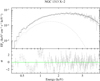 |
Fig. 12. Unfolded spectra of NGC 1313 X-2 of epoch 2017-06-20 (only pn is shown for clarity) fitted with an absorbed dual thermal component. The soft and hard diskbb components are shown with the dashed and dotted lines respectively, while the total model is shown with a solid line. Strong residuals are seen at soft energies at around 1 keV. |
Overall the variability of the source and its low pulse-fraction (∼5%) support a scenario in which NGC 1313 X-2 is a weakly magnetised NS, in which Rsph > Rm and therefore outflows and precession cause the emission to be highly anisotropic. This is also supported by the recent ray tracing Monte-Carlo simulations of Mushtukov et al. (2021), showing that larger scale-height flows lead to lower pulse-fraction due to the increased number of scatterings.
NGC 7793 P13 and M 51 ULX-7: Rm > Rsph – Conversely, both the long-term evolution of NGC 7793 P13 and M 51 ULX-7 show little variability in terms of hardness ratio, although they are also associated with super-orbital periodicities of 66.9 days (see Fürst et al. 2018, Fig. 5) in the case of NGC 7793 P13 and 39 days in the case of M 51 ULX-7 (Vasilopoulos et al. 2020). Indeed, long-term Swift-XRT monitoring shows no clear bi-modal behaviour (Weng & Feng 2018) in a hardness–intensity diagram in the case of NGC 7793 P13. Both sources also show a very hot hard component (Thard ∼ 3 keV), although it is unclear whether the absence of a third, high-energy component may have boosted the inferred temperature. In a similar way as for NGC 1313 X-2, most of the luminosity variability is again seen in the hard component (the soft component varies by a factor of about two and the hard component by a factor of about five). However, for NGC 7793 P13 and M 51 ULX-7, the soft component does seem to brighten with source luminosity.
The lack of HR variability might indicate that anisotropic emission caused by the wind funnel is not important in these sources. As stated before, in the presence of a strong magnetic field, the disk might be truncated before radiation pressure starts to be sufficient to inflate the disk and drive the strong outflow. Assuming the geometry of the accretion flow outside Rm is similar to that of supercritically accreting BHs, our soft diskbb could represent the emission from the outer regions of the accretion disk, with partial reprocessing by the wind if Rm > Rsph (Kitaki et al. 2017). If we consider this model component to provide a rough estimate of the size of this emitting region, a larger emitting area compared to NGC 1313 X-2 –for which we have argued that outflows are important– could indicate that the disk is being truncated further from the accretor in the case of NGC 7793 P13 and M 51 ULX-7. To illustrate this, we compute the mean radius of the inner disk given by the soft diskbb normalisation (N) from all epochs. Using
 (3)
(3)
where i is the inclination of the system, D10 is its distance in units of 10 kpc, and fcol is the colour correction factor (Shimura & Takahara 1995), which we take as 1.8 (e.g., Gierliński & Done 2004) throughout this paper, gives 1637 (cos i)−1/2 km, 1975
 , and 2257
 (cos i)−1/2 km for NGC 1313 X-2, M 51 ULX-7, and NGC 7793 P13, respectively. Naively assuming this radius gives a rough estimate of the size of the magnetospheric radius (Rm), it may indicate a higher mass-accretion rate for NGC 1313 X-2 (and/or a lower magnetic field strength) and thus a scenario in which the disk becomes thick and outflows cause anisotropic emission. Instead, the larger radius of NGC 7793 P13 and M 51 ULX-7 may suggest that either the mass-accretion rate is lower or the magnetic field strength is higher, which can result in the disk remaining geometrically thin (see also Chashkina et al. 2017) and therefore in reduced anisotropy. We note that these would support previous studies by Koliopanos et al. (2017), where the same relationships for Rm and Rsph were found for NGC 7793 P13 and NGC 1313 X-2 (see their Tables 2 and 4).
Assuming the mass-accretion rate varies within a similar range in the three sources, a stronger magnetic field in NGC 7793 P13 and M 51 ULX-7 is also supported by the fact both sources undergo periods of inactivity to ≲1038 erg s−1, likely associated with the propeller regime (e.g., Fürst et al. 2016; Vasilopoulos et al. 2021), indicating that the condition Rm > RC is more easily achieved. Furthermore, the lower pulse-fraction of NGC 1313 X-2 compared to that of NGC 7793 P13 and M 51 ULX-7 is consistent with less material reaching the magnetosphere and thus the accretion column, as a result of the mass loss in the disk. Therefore, the emission at high energies is not only intrinsically diminished but also down-scattered in the outflow (Mushtukov et al. 2021), which might explain why NGC 1313 X-2 is generally softer than NGC 7793 P13 and M 51 ULX-7.
We therefore suggest that the magnetic field in NGC 7793 P13 and M 51 ULX-7 is likely to be higher than that of NGC 1313 X-2, meaning that Rm > Rsph. The low degree of beaming and high magnetic field implied by this solution are in agreement with previous magnetic field estimates (Vasilopoulos et al. 2020; Rodríguez-Castillo et al. 2020) that suggested a magnetic field of ∼1013 G in M 51 ULX-7.
NGC 5907 ULX1: Rm ∼ Rsph – Contrary to the rest of PULXs in our sample, the luminosity of NGC 5907 ULX1 clearly exceeds 1040 erg s−1. The variability between the observations clustered at LX ∼ (6−8) × 1040 erg s−1 (epochs 2003 and 2014) and epoch 2012 was shown to be associated with different phases of the 78 day super-orbital period (Walton et al. 2016b) of the source by Fürst et al. (2017). This suggests that these changes are not due to a change in the mass-accretion rate and instead suggests changes in the viewing angle as the sources precesses. It has been speculated that the extreme luminosity of the source could be due to a high degree of beaming (e.g., King et al. 2017; King & Lasota 2019), in which the super-orbital modulation was due to a conical outflow beaming the emission into and out of our line of sight (e.g., Dauser et al. 2017). However, our Fig. 6 shows that the source is harder when it becomes dimmer in epoch 2012-02-09 (see also Fig. 3 from Sutton et al. 2013) compared to epochs in 2003 and 2014, and thus these changes associated with the super-orbital period may be hard to reconcile with changes imprinted by the precession of an outflowing cone, as we would expect a softer emission at low luminosities. This might imply that Rsph ≤ Rm is likely in the case of NGC 5907 ULX1.
We note that other mechanisms could also cause the luminosity to be overestimated under the assumption of isotropic emission. In reality, the emission from the accretion column is not expected to be emitted isotropically. Instead, radiation-hydrodynamic simulations of super-Eddington accretion onto magnetised NSs by Kawashima et al. (2016) show that the accretion column is expected to have a flat emission profile along its sides, as the emission is only able to escape through the lateral sides of the confined material within it. This naturally creates highly anisotropic emission and can cause the observed emission to be greatly in excess of the Eddington limit.
A high ṁ0 is still likely required to produce the observed luminosities. This may require the presence of a strong magnetic field so that the disk is truncated roughly at the point where it becomes supercritical. Thus, as suggested previously (Walton et al. 2018a; King & Lasota 2019), Rsph ∼ Rm seems a plausible condition to explain the high luminosity of NGC 5907 ULX1.
4.2. The non-pulsating NS: M 51 ULX8
This source was identified as a NS through the identification of a possible cyclotron resonance feature (Brightman et al. 2018)10. We note that its position in the HLD (see Fig. 4) may be consistent with a lack of pulsations (Brightman et al. 2018), as this source is markedly dimmer and softer than the overall PULX sample, and sources with higher pulse fractions tend to sit in the harder end of the diagram, as stated before. However, given the apparent lack of variability, it is hard to make a comparison between this source and other PULXs in our sample. Strong variability is only observed for M 51 ULX8 in epoch 2018-05-25, where the hard component increased by a factor of two in luminosity. Its behaviour is somewhat similar to that of NGC 1313 X-2 and M 81 X-6, the latter we argue is a good PULX candidate (see Sect. 4.3), although we lack enough observations of the source at higher luminosities to confirm this similarity. The soft component also shows little variability and no clear correlation, suggesting again a link between these three sources, which would favour a weakly magnetised NS in M 51 ULX8 in agreement with the study presented by Middleton et al. (2019). Should this be the case, then long-term monitoring of the source will be crucial to attempt to identify any quasi-periodicity similar to those seen in NGC 1313 X-2 and M 81 X-6.
4.3. PULX candidates
M 81 X-6 – As stated above, M 81 X-6 constitutes our best NS-ULX candidate. The spectral evolution and the track in the HLD for this source are strikingly similar to those of NGC 1313 X-2 (Fig. 6). Both sources transit back and forth from a soft (HR ≲ 1.5) and low-luminosity state (≲4 × 1039 erg s−1) to a hard (HR ∼ 3) and brighter state. The similar temperature, luminosity range, and variability (or lack of it) of the soft component also suggests a link between these two sources. Instead, the variability is driven mostly by the hard component (the soft diskbb changes by a factor ≲2 in luminosity while the hard component luminosity varies by a factor ≲5 in both sources). Furthermore, the variability of M 81 X-6 is also likely associated with a 115 day quasi-periodicity (Weng & Feng 2018) compatible with the one seen in NGC 1313 X-2. Given the similarity of these two sources, we suggest that M 81 X-6 also harbours a weakly magnetised NS, meaning that the presence of strong outflows along with source precession may account for its spectral variability.
Prompted by this similarity, we searched for coherent pulsations in M 81 X-6 using the code HENDRICS (Bachetti 2018) which is based on the publicly available Python library STINGRAY (Huppenkothen et al. 2019). Unfortunately, all but one of the observations have less than 5000 counts in pn, and typically 10 000 counts seem to be required in order to detect pulsations (Rodríguez-Castillo et al. 2020). We therefore searched in the observation with the longest exposure (∼73 ks in pn, see Table 1 and Fig. 6 epoch 2001-04-23, HR ∼ 2, L ∼ 4 × 1039 erg s−1) suitable for pulse searches, assuming M 81 X-6 has a period and period derivative similar to the other PULXs. We used the Chandra coordinates given by Swartz et al. (2003) to extract barycentred corrected events in the 0.2−12 keV band. We ran HENDRICS on the unbinned event file searching for coherent pulsations in the 0.2−8 Hz range based on previous PULX detections and using the Z2 statistic (Buccheri et al. 1983) suitable for sinusoidal pulses. The search was performed using the option fast, which optimises the search in the f − ḟ space and reduces the computational time tenfold compared to a classical search. We found no detection above the 3σ level. We ran the same search in the four longest GTI intervals, ranging from 20 ks to 40 ks, as pulsations in PULXs have been shown to vary during the course of an observation (e.g., Bachetti et al. 2020), but again we did not find any significant detections. Overall there is no peak that can be robustly identified as several peaks with similar Z2 power are found, well below the 3σ level. We also looked in the pn data of the individual observations with shorter exposures, but found no significant detections. We performed a last search looking into the 0.02−0.2 Hz range to look for longer periods as those seen in NGC 300 ULX1 (see e.g., Vasilopoulos et al. 2018), with similar results. This could indicate that pulsations in this source are as elusive and faint as those found in NGC 1313 X-2 (Sathyaprakash et al. 2019) and that deep exposures with the source on-axis or deeper searches correcting for the orbital parameters will be required to detect pulsations.
Alternatively, the spectral state of the source may play a role in the detectability of the pulsations. Considering the case of NGC 1313 X-2, the epochs when pulsations were detected by Sathyaprakash et al. (2019) are 2017-09-02 and 2017-12-09 (i.e. the last two epochs in Fig. 6). The authors also found that the pulse fraction (and hardness, as shown in this work, Fig. 4) decreases with the source luminosity. As argued before, we understand the hardening of the source as a decrease in the viewing angle as the system precesses. Considering the pulse-fraction calculations for super-critical accretion columns proposed by Inoue et al. (2020), this might imply that the angle between the rotational axis and the magnetic field axis (ΘB) is greater than the angle between the observer’s line of sight and the rotational axis (Θobs; e.g., ΘB > 30° and Θobs < 30°, see Fig. 5 from Inoue et al. 2020). Assuming the same applies to M 81-X6, this could imply that pulsations are more likely to be found in softer and dimmer states (HR ∼ 1.5, L ∼ 2.5 × 1039 erg s−1) where we expect the pulse fraction to be higher.
If, instead, the dilution of the pulsed emission is mainly due to a stochastic process such as multiple scatterings through the wind, then it may be possible to find a PULX in similar spectral states, with and without pulsations. Nevertheless, studying the dependence of the appearance of pulsations on the source spectral states seems a promising tool to put constraints on the accretion flow geometry in PULXs.
4.4. Geometrical effects of a supercritical funnel
Several of the softer sources for which the accretor is unknown show a common pattern in their long-term evolution: three distinct spectral states, two of them at similar low luminosities but distinct hardness and a third one at a higher luminosity (see e.g., NGC 1313 X-1, Circinus ULX5 and IC 342 X-1 in Fig. 6). Two other sources that also show three marked spectral states are Holmberg II X-1 and NGC 5204 X-1, although the luminosity of the dimmer states differs in this case by a factor of between approximately two and four. The difference in luminosity between one of the two dim states and the bright state might be naturally explained by changes in ṁ0. However, the presence of an additional dim state requires another explanation. A supercritical funnel, as we discuss below, may offer an explanation for these three states either through obscuration as ṁ0 increases (sources in Sect. 4.4.1) or changes in the inclination of the system (sources in Sect. 4.4.2). Given some of the common transitions and other spectral properties as we show below, we discuss NGC 1313 X-1, Holmberg IX X-1, NGC 55 ULX1, Circinus ULX5, and IC 342 X-1 together in Sect. 4.4.1 and Holmberg II X-1 and NGC 5204 X-1 in Sect. 4.4.2.
Here, we use NGC 1313 X-1 as our benchmark to discuss some of the transitions observed to the soft and dim states. In some cases, the timescale between these transitions and the duration of each state are poorly constrained because of the sparsity of our data. However, in a few cases, as for NGC 5204 X-1 and NGC 1313 X-1, the sampling rate is high enough for us to observe the source switching from one state to another and therefore we refer to these changes as transitions.
4.4.1. Optically thick funnels
NGC 1313 X-1 and Holmberg IX X-1 – As we show later, NGC 1313 X-1 undergoes a transition similar to that observed in the super-soft ULXs in NGC 247 Feng et al. (2016) and M 101 (Soria & Kong 2016), which are seen to transit from ULSs to a soft ULX spectrum. A similar transition is also seen in NGC 55 ULX1 (Pinto et al. 2017) (and in this work as we argue later), although the source would still be classified as a ULX when in this dim state. These transitions are all marked by an increase in the size of the emitting region of the soft component and a decrease in temperature, interpreted as an expansion of the wind photosphere as the spherisation radius increases with the corresponding decrease in temperature (Poutanen et al. 2007). While the ULXs in M 101 and NGC 247 are frequently thought to be viewed at high inclinations (e.g., Ogawa et al. 2017), NGC 1313 X−1 is likely viewed down the optically thin funnel (e.g., Poutanen et al. 2007; Narayan et al. 2017), so that the hard component dominates the emission (epoch 2012-12-16 in Fig. 6).
The spectral transitions of NGC 1313 X-1 between the low state (L ∼ 8 × 1039 erg s−1, epoch 2012-12-06) and the high state (L ∼ 18 × 1039 erg s−1, epoch 2004-06-05) have been frequently interpreted as the wind entering our line due to a narrowing of the funnel as the mass-accretion rate increases (e.g., Sutton et al. 2013). However, the fact that the high-energy emission (≳10 keV) remains relatively stable may be at odds with this interpretation, as we should expect the wind to down-scatter (Kawashima et al. 2012; Middleton et al. 2015b) or even absorb (Abolmasov et al. 2009) the high-energy emission from the inner parts of the accretion flow. We should also expect the increase in the mass-transfer rate to lead to an increase in the Thomson scattering optical depth of the funnel (Kawashima et al. 2012), also causing the high-energy emission to drop.
The physical processes at play to produce these high-energy photons are still poorly understood (e.g., Walton et al. 2020) but it is generally accepted that this emission is produced in the vicinity of the accretor (e.g., Kawashima et al. 2012; Takahashi et al. 2016; Walton et al. 2020). For the remainder of this part, we assume that this high-energy component is indeed produced in the inner regions of the accretion flow and focus on the influence of the wind and funnel structure on the spectra, rather than on the origin of this emission, which is discussed in Sect. 4.5.
The fact that the high-energy component remains stable could therefore imply that the gas within the funnel has remained optically thin over a certain range of mass-transfer rate, and that the inclination of the system (i) remains well below the half-opening angle of the funnel (θf). The second condition is required so that the higher degree of beaming caused by the reduction of θf, will only result in an increase in the amount of photons that are down-scattered off the wind walls into the observer’s line of sight, with the wind remaining out of the line of sight. As the optical depth of the wind is lowest near the rotational axis of the compact object (Poutanen et al. 2007), the emission from the innermost regions is more likely to reach the observer without suffering severe energy losses (Kawashima et al. 2012). This may support the conclusions of previous works suggesting that NGC 1313 X-1 is seen at low viewing angles (e.g., Middleton et al. 2015b).
The lack of obscuration of the high-energy emission suggests that the mass-accretion rate has to be moderate (Ṁ ≲ 10 ṀEdd)11 as for higher mass-transfer rates the gas within the funnel is expected to become optically thick (Narayan et al. 2017). Therefore, regardless of the exact nature of this high-energy power-law tail, we argue that despite the increase in mass-accretion rate in NGC 1313 X-1 up to epoch 2004-06-05, the physical conditions within the funnel have remained stable. The similar persistent high-energy emission seen in Holmberg IX X–1 and the similar L–T positive correlation suggest a similar evolution in both sources, although NGC 1313 X–1 is seen in an obscured state (see below) not seen in Holmberg IX X–1. We discuss the possible differences between these two sources in more detail in Sect. 4.5, focussing on the nature of the high-energy tail.
Interestingly, after NGC 1313 X–1 reaches its maximum luminosity (epoch 2004-06-05), it becomes extremely soft and its luminosity decreases (epoch 2004-08-23 – obscured state). This spectral transition (we note that these two observations are just two months apart) can be understood if a further increase in the mass-accretion rate leads to a narrowing of the opening angle of the funnel as the wind becomes more mass loaded, to the point where the gas within the funnel becomes optically thick to the high-energy radiation. This implies that now θf < i and thus the wind effectively enters the line of sight and starts obscuring the inner accretion flow. The optical depth of the wind in the direction parallel to the disk is also expected to be an order of magnitude higher than in the perpendicular direction (Poutanen et al. 2007). High-energy photons are now heavily down-scattered or absorbed and therefore we mostly observe the soft emission from the expanded wind photosphere, as supported by the increase in the normalisation of the soft component (from ∼5 to ∼50 before and after the obscuration respectively).
This transition is also in good agreement with the GRRMHD simulations presented by Narayan et al. (2017) of super-Eddington accretion onto BHs. The authors observe a transition from a hard spectrum to a very soft one, as the mass accretion rate increases (Ṁ ∼ 23 ṀEdd from their simulations) and the gas within the funnel becomes optically thick (see their Fig. 9). Furthermore, their simulations also show that the luminosity for an observer with a line of sight close to the rotational axis of the accretor (i ∼ 10°) is capped at around 2 × 1040 erg s−1, which is in very good agreement with the maximum luminosity observed in NGC 1313 X-1. Their simulations also predict an increase in the spectral emission at low energies (≲0.6 keV), which seem at odds with our observations, where the luminosity of the soft component has remained stable compared to the brightest state. However, we note that Kawashima et al. (2012), who found qualitatively the same results as Narayan et al. (2017) for high-mass transfer rates (≳23 ṀEdd), do not observe an increase in luminosity at low energies. It is also possible that because of the expansion of the photosphere, the soft component peaks now in the extreme UV and therefore we cannot reliably assess whether the luminosity of the soft component has increased given our limited bandpass.
Numerical simulations by Ogawa et al. (2017) also predict a steep decline in the high-energy emission as the outflow photosphere enters the line of sight. We find that the temperature of the hard diskbb diminishes from 1.6 ± 0.1 keV in epoch 2004-06-05 to 0.92 keV in epoch 2004-08-23 and its unabsorbed bolometric luminosity decays from (11.2 ± 0.6) × 1039 erg s−1 to (2.9 ± 0.4) × 1039 erg s−1, which seems to support this interpretation.
NGC 55 ULX1 – Similarly, we argue that the soft and dim spectral state observed in NGC 55 ULX1 is analogous to the obscured state observed in NGC 1313 X-1. In both cases, we observe a possible increase in the neutral absorption column (see Sect. 3.1.2). Although this might be model dependent (this is discussed further below), it suggests that their spectra have evolved in a similar manner. The ratio of unabsorbed bolometric fluxes in the obscured state are Fhard diskbb/Fsoft diskbb = 0.34 and 0.29
 in NGC 1313 X-1 (epoch 2004-08-23) and NGC 55 ULX1 (epoch 2010-05-24), respectively. This is a factor of about three lower in both cases compared to when the sources were at their brightest, and indicates that the hard component is responsible for the drop in luminosity. We again see an increase in the normalisation of the soft diskbb (see also Pintore et al. 2015) akin to the transitions seen in the ULXs in M 101 and NGC 247 (Feng et al. 2016; Soria & Kong 2016). The increase in the neutral absorption column may indicate that now we see parts of the wind less exposed to the central source (Pinto et al. 2020a), where self-absorption could start to be important, although more physically motivated models are needed to address this. The presence of outflows is supported by studies using high-resolution spectroscopy (Pinto et al. 2017, 2020b) which might have revealed the presence of soft residuals associated with outflowing winds in NGC 1313 X-1 and NGC 55 ULX1. Their similar transitions highlighted here therefore support the unification scenario proposed by (Middleton et al. 2015b; Pinto et al. 2020a).
IC 342 X-1 and Circinus ULX5 – As shown in Fig. 6, IC 342 X-1 and Circinus ULX5 not only share a very similar evolution in the HLD, but are also found in a soft and dim state (epochs 2012-10-29 and 2016-08-23 for IC 342 X-1 and Circinus ULX5 respectively) reminiscent again of the obscured state seen in NGC 1313 X-1. When both sources are hard and dim (e.g., epochs 2012-08-07 and 2001-08-06 for IC 342 X-1 and Circinus ULX5 respectively) the mass-transfer rate is likely to be low, similar to that of NGC 1313 X-1 in epoch 2012-12-16. The brighter and harder states (epochs 2005-02-10 and 2013-02-30 for IC 342 X-1 and Circinus ULX5 respectively) might correspond to an increase in the mass-transfer rate while the softest and dimmest states are likely again due to the central source being obscured by the funnel becoming optically thick at high-transfer rates. This is supported by the diminishing of the hard component in both temperature and luminosity. In this case, we do not see an increase in the local nH-value as for NGC 1313 X-1 or NGC 55 ULX1, which could strengthen the similarities of these obscured states, but we note that these are the two sources with the largest nH Gal-values (≳30 × 1020 cm−2) in our sample and that we noted some calibration uncertainties at low energies (see Sect. 2.2). Nevertheless, these sources show that both archetypal soft ULXs (e.g., NGC 55 ULX1) and hard ULXs (e.g., IC 342 X-1) undergo a similar type of transition.
4.4.2. Inclination effects
Holmberg II X-1 and NGC 5204 X-1 – The similarities between Holmberg II X-1 and NGC 5204 X-1 are clear when looking at their long-term evolution in the HLD (see also the similarity between the three spectra shown in Fig. 6) and are further supported by the similar L–T correlations found for the soft diskbb (αNGC 5204 X − 1 = 3.6 ± 0.4, αHolmberg II X − 1 = 3.3 ± 0.4). Therefore, regardless of the physical processes powering these two sources, these similarities strongly suggest that we are witnessing the same type of source and/or accretion flow (see also Gúrpide et al., in prep.).
In epochs 2004-04-15 and 2006-11-16 of Holmberg II X-1 and NGC 5204 X-1 respectively, both sources are found with a hard spectrum and an intermediate luminosity – hard/intermediate state. Again, we favour a low viewing angle for NGC 1313 X-1 as the hard component dominates the emission, although the inclination in this case may be higher than for NGC 1313 X-1 given their softer spectra. As both these sources move in the HLD (see 2003 XMM-Newton epochs for NGC 5204 X-1 for the transition) from these epochs to softer spectra and brighter luminosities – bright/soft state (e.g., epochs 2004-04-15 and 2006-11-16 for Holmberg II X-1 and NGC 5204 X-1 respectively)–, the temperature of the hard component decreases as seen in NGC 1313 X-112, while the soft component increases in temperature and luminosity (see Table 2). Similarly, most of the variability between these two epochs is seen at mid to soft energies (∼0.3−5 keV), whereas the high-energy emission (≳5 keV) shows little variability. We argue that these transitions are due once again to an increase in the mass-accretion rate as the slight softening of both sources at high energy and the increase in the soft component seem to match the evolution presented by Kawashima et al. (2012) (see their Fig. 2). In this case, the small dimming seen at high energies (≳10 keV; see especially spectra for Holmberg II X-1) may be due to the fact that our line of sight may now be grazing the optically thick walls of the wind, and thus some of the high-energy photons from the inner parts of the accretion flow are now being Compton down-scattered by the wind. The transitions from hard/intermediate to soft/bright in NGC 5204 X-1 were also reported by Sutton et al. (2013) in terms of hard and soft ULX transitions.
Our study shows that these sources are also seen to transit from bright/soft to another state that we term dim/soft (epochs 2002-09-18 and 2001-05-02 for Holmberg II X-1 and NGC 5204 X-1 respectively) and vice versa. For NGC 5204 X-1, this is also seen in the Chandra observations of 2003 (see also the full set of Chandra observations presented by Roberts et al. 200613). For Holmberg II X-1, this is also seen in 2010 (see also the 2009/2010 Swift-XRT monitoring of Holmberg II X-1 in Grisé et al. 2010).
While there are certain similarities between these transitions and that seen in NGC 1313 X-1 in the obscured state, namely a softening and dimming of the source, we also find certain differences that may indicate that these transitions are not due to the same phenomenon as for NGC 1313 X-1. From the bright/soft state to the dim/soft state, the entire spectrum seems to have diminished in luminosity in the case of Holmberg II X-1 and NGC 5204 X-1 (see the spectra from Fig. 6), while for NGC 1313 X-1 we show that it was the hard component that is mostly responsible for the dimming. Indeed, the soft diskbb is the faintest in the dim/soft state, while the temperature of the hard diskbb remains consistent within errors with respect to the bright/soft state (for both Holmberg II X-1 and NGC 5204 X-1). If the funnel has become optically thick due to an increase in the mass-transfer rate and is now obscuring the hard emission, we should expect the soft component to be relatively stable as seen in NGC 1313 X-1. Therefore, the dimming of this component may be at odds with this interpretation.
It is worth noting that the spectral evolution of NGC 5204 X-1 and Holmberg II X-1 from bright/soft to dim/soft bears some resemblance with how the inclination affects the spectral shape (see e.g., Kawashima et al. 2012; Kitaki et al. 2017; Narayan et al. 2017), which could suggest that changes in the inclination are responsible for these spectral changes. Indeed, numerical simulations by Narayan et al. (2017) predict a decrease by about one order of magnitude in luminosity between a source with a face-on aspect and a source viewed at high inclinations (i > 30°), which is consistent with our observations of the transitions from bright/soft to dim/soft. However, if the inclination of the system is indeed changing because of precession of the supercritical funnel, we should expect these changes to be associated with some periodicity. Thus, the fact that these transitions do not seem to be periodic (Grisé et al. 2010) may be at odds with the effects of a precessing funnel (albeit see Gúrpide et al., in prep.).
These transitions were also shown to occur rapidly, in some cases on timescales shorter than half a day (Grisé et al. 2010). This short-term variability may be expected if dense clumps of the wind are intersecting our line of sight (Takeuchi et al. 2013; Middleton et al. 2015b) or if our line of sight is rapidly changing between seeing down the funnel and seeing through the wind walls, which is expected if our line of sight grazes the wind as argued above. More information on and monitoring of the timescale of these transitions is needed to address this issue and therefore this will be further studied in a forthcoming publication.
4.5. Origin of the high-energy tail
As stated above, NGC 1313 X-1 and Holmberg IX X-1 show a remarkably stable emission above ∼8 keV, although the sources are clearly varying at lower energies. Several physical processes have been proposed to explain the high-energy emission in ULXs; here we attempt to discuss its nature based on this observed stability.
Crucially, the absence of a hard surface in BHs naturally offers an explanation for the presence of a stable emission component: advection and photon trapping effects (Abramowicz et al. 1988; Ohsuga & Mineshige 2007). In the super-Eddington regime, the diffusion photon time in the vicinity of the BH is expected to be greater than the accretion timescale, while part of the excess energy will go into powering the outflow, so that the luminosity only increases logarithmically with the mass-transfer rate (Poutanen et al. 2007):
 (4)
(4)
where x = 1 if only advection is considered or x = 0.6 if all the energy goes into powering the wind. Theoretical works show that this can lead to saturation of the continuum in the hard X-ray band for SMBHs (Feng et al. 2019) and therefore this stability at high-energies may provide a way of differentiating BH- from NS-ULXs, as NSs have no means of swallowing any excess energy. Therefore, if we assume the high-energy emission is rather insensitive to ṁ0 as suggested by the stability of the high-energy component in Holmberg IX X-1 and NGC 1313 X-1, we suggest that the former might harbour a heavier BH than the latter given its brighter high-energy component (around a factor ∼1.6).
Alternatively, Kawashima et al. (2012) and Kitaki et al. (2017), based on numerical radiation hydrodynamic (RHD) simulations of super-Eddington accretion onto BHs, showed that an overheated region (T ∼ 8 keV) is formed in the vicinity of the BH, where a shock is produced in the region where the outflow collides with the inflow. Photons from the disk entering this overheated region will gain energy through multiple Compton up-scatterings prior to escaping through the funnel or the wind itself (where they will undergo Compton down-scattering). Photons escaping mostly through the funnel will be less affected by Compton down-scattering and will be observed as a high-energy power-law tail in the spectrum. Kitaki et al. (2017) argued that the temperature of this region is independent of the BH mass, resulting in a similar spectral shape for the high-energy tail regardless of the BH mass. Therefore, provided that the mass-transfer rate between two given sources is similar, the luminosity of this high-energy component may provide a means to estimate the BH mass ratio between two given sources. The two sources for which this stability is best observed, NGC 1313 X-1 and Holmberg IX X-1, indeed show a similar slope for the hard tail, ΓNGC 1313 X − 1 = 2.90 , Γ1Holmberg IX X − 1 = 2.9
 , and Γ2Holmberg IX X − 1 = 3.4
 where 1 and 2 indicate the two different Γ values we used for the low- and high-flux epochs, respectively. If we instead refit all the high-quality data sets of Holmberg IX X-1 assuming one single value for Γ tied between all epochs, we obtain Γ = 3.1 ± 0.2 with
  = 1.06 for 3722 degrees of freedom, consistent with the slope found in NGC 1313 X-1. Therefore, the brighter luminosity of the high-energy component in Holmberg IX X-1 would again suggest that Holmberg IX X-1 harbours a heavier BH compared to NGC 1313 X-1.
It is however not clear yet how the physical properties of this overheated region change with the mass-transfer rate. Assuming the overheated region is indeed responsible for the stable high-energy tail, then its physical properties should also be rather insensitive to the mass-transfer rate. Given that the overheated region is formed because of the shock of the outflows colliding with the inflow, we may also expect one to form around weakly magnetised NSs too. However, it remains to be seen whether or not the physical conditions within this overheated region and the funnel can lead to the formation of a similar high-energy power-law tail as predicted for supercritically accreting BHs.
Lastly, in the case of accretion onto NS magnetic poles, the accretion column is expected to be responsible for the emission at high energies (Walton et al. 2018a). Unfortunately, simulated spectra from super-critically accreting NSs from numerical simulations are still under study (e.g., Takahashi & Ohsuga 2017; Takahashi et al. 2018) and it is currently hard to know how the emission from the accretion column reacts to changes in the mass-transfer rate and magnetic field strength. Nevertheless, if the accretion column is responsible for the stable emission observed in these sources, it is still unclear why we observe this difference in terms of stability between PULXs and sources like NGC 1313 X-1 and Holmberg IX X-1.
4.6. M 83 ULX1: a stellar-mass black hole?
This source sits at the lower end of the ULX luminosity distribution. We found the maximum unabsorbed luminosity of M 83 ULX1 to be ∼3.5 × 1039 erg s−1, close to the maximum observed luminosity of ∼4.5 × 1039 erg s−1 by Soria et al. (2015), although this was computed using a power law which could have boosted the unabsorbed luminosity. This maximum luminosity, using Eddington mass scaling, suggests an accretor of ∼25 M⊙. We also found that the hard diskbb component follows Lhard ∝  , which, as suggested by Fig. 10, does not seem to be spuriously created by existing degeneracies. This may suggest that this component arises from an accretion disk with constant inner radius. This fact together with its low maximum luminosity, may suggest that we are witnessing a BH accreting close to the Eddington-limit, as binary synthesis population studies predict that BH-ULXs tend to emit isotropically, because super-Eddington mass-transfer rates (a factor of approximately eight above the classical Eddington limit) are harder to obtain from binary population evolution in the case of BHs (Wiktorowicz et al. 2019).
We therefore consider the possibility that the source could be accreting close to the Eddington-limit. If so, then we could expect the accretion disk to deviate from the standard thin accretion disk as radiation pressure inflates the disk making it geometrically slim or thick. This may lead to a departure of the radial temperature index (p) of −0.75 for a standard thin accretion disk (Shakura & Sunyaev 1973), implicitly assumed in the diskbb model. In order to explore such deviations, we refitted all our data with an absorbed broadened disk model (diskpbb in XSPEC). As in Sect. 3, we assumed again constant absorption column and we jointly fitted our data tying nH across all datasets with the diskpbb model. We obtained an excellent fit with χ2 ∼ 1.02 for 1493 degrees of freedom (parameters are listed in Table 6).
Results from jointly fitting all datasets of M 83 ULX1 with an absorbed diskpbb model.
Results of the F-test between tbabs⊗tbabs⊗(diskbb + diskbb) (1) and tbabs⊗tbabs⊗(diskbb + simpl⊗diskbb) (2) models.
The overall evolution of M 83 ULX1 is very similar to that seen in the ∼10 M⊙ BH XTE J1550–564 (Kubota & Makishima 2004). Our hard diskbb when using the dual-thermal component shows constant inner-disk radius, closely following the L ∝ T4 relationship as XTE J1550–564 in the standard regime (i.e. when Ldisk ∝ T4; e.g., period 3 in Kubota & Makishima 2004)14. Additionally, when using the diskpbb model, the temperature increases with the radial index p of the diskpbb (Fig. 13) as seen in XTE J1550–564 and LMC X-3 when fitted with the same model (see their Fig. 9). Kubota & Makishima (2004) argued that this increase in p with temperature is an artefact caused by the limited bandpass and the fact that the radial dependency is flatter near the innermost disk radius than the −0.75 given by the diskbb approximation. Our diskpbb L–T relationship follows α = 3.0 ± 0.6 (90% confidence level) with Spearman’s test coefficient of 0.94, again with roughly constant normalisation, suggesting that we are witnessing the innermost stable orbit as in XTE J1550–564 and LMC X-3 in the standard regime. A typical value of the normalisation N ∼ 0.002, corresponds to Rin ∼ 95 (cos i)−1/2 km, assuming fcol = 1.8 as above. If we assume that the constant radius we observe corresponds to the innermost stable orbit for a non-spinning BH, then Rin = Risco = 3RS, and we obtain a BH mass estimate of ∼10 (cos i)−1/2 M⊙. This mass estimate would be a factor of six larger if we consider instead a maximally spinning Kerr BH.
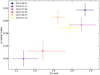 |
Fig. 13. Dependency of the p radial index of the diskpbb with its temperature for M 83 ULX1 (see text for details). This dependency is similar to that seen in SMBHs in the standard regime (Kubota & Makishima 2004). Symbols are as per Fig. 7. |
A further constraint on the mass of the BH comes from the fact that Kubota & Makishima (2004) argued that a source enters the anomalous regime when Ldiskb/LEdd ∼ 0.4. Therefore, given that Ldisk ∼ 4 × 1039 erg s−1, then the mass of the M 83 ULX1 could be of the order of 60 M⊙, which could easily be accounted for with reasonable values of inclination and spin of the BH. We note that it is unlikely that the source is in the anomalous state as we should expect p to decrease with temperature, as this parameter starts to deviate from the standard value for a thin disk of −0.75 (Kubota & Makishima 2004; Shakura & Sunyaev 1973), which is at odds with our observations (Fig. 13).
Although the exact mass estimate is rather uncertain, we conclude that the behaviour of this source is consistent with a massive SMBH accreting close to the Eddington limit in the high/soft state, given its similar evolution with accreting BHs in the standard regime. This conclusion is in agreement with previous studies by Soria et al. (2015) and other studies suggesting that sources below 3 × 1039 erg s−1 could be consistent with massive BHs accreting close to the Eddington limit (Middleton et al. 2013; Sutton et al. 2013). Such massive BHs might not be rare given the BH masses estimated from gravitational wave events (Abbott et al. 2019).
5. Conclusions
We present a thorough study of the long-term spectral evolution of a representative sample of ULXs and PULXs using data from XMM-Newton, Chandra, and NuSTAR. By studying their spectral states and transitions, we are able to explain the main sources of variability in these sources, which can be summarised as changes in the mass-transfer rate, changes in the degree of beaming, precession, and obscuration by the optically thick parts of the wind as this latter becomes more mass loaded.
We show that PULXs are among the hardest sources in the sample and discuss their evolution in terms of the interplay between the magnetospheric radius and the spherisation radius. We favour a scenario in which the softest PULX, NGC 1313 X-2, is consistent with a weakly magnetised NS so that Rsph > Rm and the wind/funnel structure is responsible for imprinting highly anisotropic emission as the source precesses, given the wide HR variability the source spans. This interpretation can explain the significantly softer spectra of NGC 1313 X-2 and its lower pulse fraction, as the primary emission from the accretion column is expected to be down-scattered in the cool electrons of the outflow. Additionally, the lack of transitions to the propeller regime in NGC 1313 X-2 supports this interpretation, as the weak magnetic field (or high-mass transfer rate) implied by the condition Rsph > Rm will naturally lead to smaller magnetospheric radii, making transitions to the propeller regime less likely to occur. Instead, the hardest PULXs, NGC 7793 P13 and M51-ULX7, are consistent with being strongly magnetised, meaning that Rm > Rsph given the lack of HR variability, which we interpret as lack of strong anisotropy. In this scenario, the accretion disk is being truncated before it becomes supercritical, suppressing the anisotropy that the funnel/wind structure would otherwise imprint. For NGC 5907 ULX1, we show that in epochs associated with the super-orbital variability, the source appears harder when dimmer. This is hard to reconcile with the anisotropy expected from the funnel/wind structure in which we expect the source to become harder when brighter (as for NGC 1313 X-2). Still, a high-mass transfer rate is required to explain its high luminosity and therefore we conclude that Rsph ∼ Rm is a plausible condition to explain the source variability.
By comparing the evolution of PULXs with the sources in our sample, we are able to identify a strong NS candidate with very similar evolution to that seen in NGC 1313 X-2: M 81 X-6. Although we are not able to detect pulsations in the source, it is possible that longer exposures sampling the source in different spectral states may be needed to detect pulsations. Additionally, deeper pulse searches taking into account orbital parameters corrections may be needed.
Most of the softer sources for which the accretor is unknown show three markedly different spectral states: one at highest luminosity and two at similar low luminosities but different hardness ratio. A supercritical funnel can offer an explanation of such degeneracy between luminosity and hardness, because a source is expected to be dim at both low mass-transfer rates and when the gas within the funnel becomes optically thick at high mass-transfer rates, causing the hard radiation from the inner regions of the accretion flow to be abruptly obscured. This could explain the evolution seen in NGC 1313 X-1, NGC 55 ULX1, IC 342 X-1, and Circinus ULX5. For Holmberg II X-1 and NGC 5204 X-1, these transitions may be better explained if our line of sight is grazing the half-opening angle of the funnel, so that our view of the accretion flow rapidly transits between seeing down the funnel and seeing through the optically thick wind walls as the source precesses. Future higher cadence monitoring of these transitions will be key to determining the exact nature of these transitions, by studying both their timescale and the source evolution preceding and following them. Nevertheless, these transitions are suggestive of strong winds in these sources, which together with their softer appearance compared to most PULXs supports a scenario in which the sources considered here are powered by weakly magnetised NSs or BHs.
Finally, we report on the stability of the high-energy emission (≳10 keV) in some of the sources in our sample. Notably, none of the PULXs show such stability, although further high-quality NuSTAR observations are needed to probe the different spectral states of both PULXs and those sources for which the accretor is unknown. BHs are favoured candidates to explain this stability, as they naturally offer a means to swallow any excess radiation, stabilising the output radiation even as the mass-transfer rate increases. Should this be the case, this high-energy emission may help to identify BH-ULXs. On the other hand, should some of these sources host NSs, then this stability may offer interesting clues about the accretion flow geometry around NSs in the super-Eddington regime. Nevertheless, we stress the importance of obtaining future NuSTAR observations as we may expect to see most of the observational differences between BH- and NS-ULXs at high energies, where the mechanism responsible for the emission is expected to differ (i.e. an accretion column compared to the case of the inner regions of the accretion disk around a BH).
For the jointly fitted data, this flux calculation is done taking into account errors associated with all tied parameters.
We note that the increase in luminosity of NGC 5408 X-1 in 2001 is less certain given the short exposure of the 2001 observations and our assumption of constant nH.
We note that epochs 2003-01-15 and 2013-11-25 of NGC 7793 P13 and M 51 ULX-7, where the sources are found in a softer and dimmer state, are likely associated with the sources resuming from the propeller regime.
Chandra obs id 13813, where the putative line was identified by Brightman et al. (2018) was not considered in this work due to a certain degree of pile-up affecting the observation.
Here we adopt the definition of Ṁ of Narayan et al. (2017) where Ṁ =  and η depends on the BH spin.
For NGC 5204 X-1, see those epochs of higher quality as the epochs when simpl was not included tend to appear with artificially hotter temperatures for the hard diskbb.
Although these transitions were well sampled by Chandra at the end of 2003, we were not able to use the short exposure (∼5 ks) observations when the source was caught repeatedly in the low state given the limited number of counts registered.
We note that Kubota & Makishima (2004) uses RXTE that covers the 3−20 keV range and thus their soft component corresponds roughly to our hard component.
Acknowledgments
The authors would like to thank the anonymous referee for his comments and suggestions that helped improve the quality of the manuscript. A. Gúrpide would like to thank M. Bachetti for his help and assistance during the search of pulsations and to I. Pastor-Marazuela for the computational resources provided. NW acknowledges support by the CNES. This work made used of the free software Veusz developed by J. Sanders to produce some of the plots.
References
- Abbott, B. P., Abbott, R., Abbott, T. D., et al. 2019, ApJ, 882, L24 [NASA ADS] [CrossRef] [Google Scholar]
- Abolmasov, P., Karpov, S., & Kotani, T. 2009, PASJ, 61, 213 [NASA ADS] [CrossRef] [Google Scholar]
- Abramowicz, M. A., Czerny, B., Lasota, J. P., & Szuszkiewicz, E. 1988, ApJ, 332, 646 [Google Scholar]
- Arnaud, K. A. 1996, ASP Conf. Ser., 101, 17 [Google Scholar]
- Bachetti, M. 2018, Astrophysics Source Code Library [record ascl:1805.019] [Google Scholar]
- Bachetti, M., Rana, V., Walton, D. J., et al. 2013, ApJ, 778, 163 [NASA ADS] [CrossRef] [Google Scholar]
- Bachetti, M., Harrison, F. A., Walton, D. J., et al. 2014, Nature, 514, 202 [NASA ADS] [CrossRef] [Google Scholar]
- Bachetti, M., Maccarone, T. J., Brightman, M., et al. 2020, ApJ, 891, 44 [CrossRef] [Google Scholar]
- Basko, M. M., & Sunyaev, R. A. 1976, MNRAS, 175, 395 [NASA ADS] [CrossRef] [Google Scholar]
- Brightman, M., Harrison, F., Walton, D. J., et al. 2016, ApJ, 816, 60 [Google Scholar]
- Brightman, M., Harrison, F. A., Fürst, F., et al. 2018, Nat. Astron., 2, 312 [NASA ADS] [CrossRef] [Google Scholar]
- Brightman, M., Earnshaw, H., Fürst, F., et al. 2020, ApJ, 895, 127 [CrossRef] [Google Scholar]
- Buccheri, R., Bennett, K., Bignami, G. F., et al. 1983, A&A, 128, 245 [NASA ADS] [Google Scholar]
- Cappellari, M., Emsellem, E., Krajnović, D., et al. 2011, MNRAS, 413, 813 [NASA ADS] [CrossRef] [Google Scholar]
- Carpano, S., Haberl, F., Maitra, C., & Vasilopoulos, G. 2018, MNRAS, 476, L45 [NASA ADS] [CrossRef] [Google Scholar]
- Casares, J., Jonker, P. G., & Israelian, G. 2017, Handbook of Supernovaev (Cham: Springer), 1499 [Google Scholar]
- Chashkina, A., Abolmasov, P., & Poutanen, J. 2017, MNRAS, 470, 2799 [NASA ADS] [CrossRef] [Google Scholar]
- Chashkina, A., Lipunova, G., Abolmasov, P., & Poutanen, J. 2019, A&A, 626, A18 [NASA ADS] [CrossRef] [EDP Sciences] [Google Scholar]
- Colbert, E. J. M., & Mushotzky, R. F. 1999, ApJ, 519, 89 [NASA ADS] [CrossRef] [Google Scholar]
- Crook, A. C., Huchra, J. P., Martimbeau, N., et al. 2007, ApJ, 655, 790 [Google Scholar]
- Dauser, T., Middleton, M., & Wilms, J. 2017, MNRAS, 466, 2236 [NASA ADS] [CrossRef] [Google Scholar]
- Done, C., & Gierliński, M. 2003, MNRAS, 342, 1041 [NASA ADS] [CrossRef] [Google Scholar]
- Farrell, S. A., Webb, N. A., Barret, D., Godet, O., & Rodrigues, J. M. 2009, Nature, 460, 73 [NASA ADS] [CrossRef] [PubMed] [Google Scholar]
- Feng, H., & Kaaret, P. 2006, ApJ, 650, L75 [NASA ADS] [CrossRef] [Google Scholar]
- Feng, H., & Kaaret, P. 2009, ApJ, 696, 1712 [CrossRef] [Google Scholar]
- Feng, H., & Kaaret, P. 2010, ApJ, 712, L169 [NASA ADS] [CrossRef] [Google Scholar]
- Feng, H., Tao, L., Kaaret, P., & Grisé, F. 2016, ApJ, 831, 117 [NASA ADS] [CrossRef] [Google Scholar]
- Feng, J., Cao, X., Gu, W.-M., & Ma, R.-Y. 2019, ApJ, 885, 93 [Google Scholar]
- Fürst, F., Walton, D., Harrison, F., et al. 2016, ApJ, 831, L14 [NASA ADS] [CrossRef] [Google Scholar]
- Fürst, F., Walton, D. J., Stern, D., et al. 2017, ApJ, 834, 77 [NASA ADS] [CrossRef] [Google Scholar]
- Fürst, F., Walton, D. J., Heida, M., et al. 2018, A&A, 616, A186 [NASA ADS] [CrossRef] [EDP Sciences] [Google Scholar]
- Ghosh, P., & Lamb, F. K. 1978, ApJ, 223, L83 [NASA ADS] [CrossRef] [Google Scholar]
- Ghosh, P., Lamb, F. K., & Pethick, C. J. 1977, ApJ, 217, 578 [NASA ADS] [CrossRef] [Google Scholar]
- Gierliński, M., & Done, C. 2004, MNRAS, 347, 885 [NASA ADS] [CrossRef] [Google Scholar]
- Gladstone, J. C., Roberts, T. P., & Done, C. 2009, MNRAS, 397, 1836 [NASA ADS] [CrossRef] [Google Scholar]
- Godet, O., Barret, D., Webb, N. A., Farrell, S. A., & Gehrels, N. 2009, ApJ, 705, L109 [NASA ADS] [CrossRef] [Google Scholar]
- Godet, O., Plazolles, B., Kawaguchi, T., et al. 2012, ApJ, 752, 34 [NASA ADS] [CrossRef] [Google Scholar]
- Gonçalves, A. C., & Soria, R. 2006, MNRAS, 371, 673 [NASA ADS] [CrossRef] [Google Scholar]
- Grisé, F., Kaaret, P., Feng, H., Kajava, J. J. E., & Farrell, S. A. 2010, ApJ, 724, L148 [NASA ADS] [CrossRef] [Google Scholar]
- Grisé, F., Kaaret, P., Corbel, S., Cseh, D., & Feng, H. 2013, MNRAS, 433, 1023 [NASA ADS] [CrossRef] [Google Scholar]
- Harrison, F. A., Craig, W. W., Christensen, F. E., et al. 2013, ApJ, 770, 103 [Google Scholar]
- HI4PI Collaboration (Bekhti, N. B., et al.) 2016, A&A, 594, A116 [NASA ADS] [CrossRef] [EDP Sciences] [Google Scholar]
- Huppenkothen, D., Bachetti, M., Stevens, A. L., et al. 2019, ApJ, 881, 39 [CrossRef] [Google Scholar]
- Illarionov, A. F., & Sunyaev, R. A. 1975, A&A, 39, 185 [NASA ADS] [Google Scholar]
- Inoue, A., Ohsuga, K., & Kawashima, T. 2020, PASJ, 72, 34 [Google Scholar]
- Israel, G. L., Belfiore, A., Stella, L., et al. 2017a, Science, 355, 817 [NASA ADS] [CrossRef] [Google Scholar]
- Israel, G. L., Papitto, A., Esposito, P., et al. 2017b, MNRAS, 466, L48 [NASA ADS] [CrossRef] [Google Scholar]
- Jansen, F., Lumb, D., Altieri, B., et al. 2001, A&A, 365, L1 [NASA ADS] [CrossRef] [EDP Sciences] [Google Scholar]
- Kaaret, P., Feng, H., & Roberts, T. P. 2017, ARA&A, 55, 303 [Google Scholar]
- Kajava, J. J. E., & Poutanen, J. 2009, MNRAS, 398, 1450 [NASA ADS] [CrossRef] [Google Scholar]
- Kalberla, P. M. W., Burton, W. B., Hartmann, D., et al. 2005, A&A, 440, 775 [NASA ADS] [CrossRef] [EDP Sciences] [Google Scholar]
- Karachentsev, I. D., Dolphin, A. E., Geisler, D., et al. 2002, A&A, 383, 125 [NASA ADS] [CrossRef] [EDP Sciences] [Google Scholar]
- Karachentsev, I. D., Kaisina, E. I., & Kashibadze Nasonova, O. G. 2017, AJ, 153, 6 [NASA ADS] [CrossRef] [Google Scholar]
- Kawashima, T., Ohsuga, K., Mineshige, S., et al. 2012, ApJ, 752, 18 [NASA ADS] [CrossRef] [Google Scholar]
- Kawashima, T., Mineshige, S., Ohsuga, K., & Ogawa, T. 2016, PASJ, 68, 83 [NASA ADS] [CrossRef] [Google Scholar]
- King, A. R. 2009, MNRAS, 393, L41 [NASA ADS] [Google Scholar]
- King, A., & Lasota, J.-P. 2016, MNRAS, 458, L10 [Google Scholar]
- King, A., & Lasota, J.-P. 2019, MNRAS, 485, 3588 [NASA ADS] [CrossRef] [Google Scholar]
- King, A., & Lasota, J.-P. 2020, MNRAS, 494, 3611 [CrossRef] [Google Scholar]
- King, A. R., & Pounds, K. A. 2003, MNRAS, 345, 657 [NASA ADS] [CrossRef] [Google Scholar]
- King, A. R., Davies, M. B., Ward, M. J., Fabbiano, G., & Elvis, M. 2001, ApJ, 552, L109 [NASA ADS] [CrossRef] [Google Scholar]
- King, A., Lasota, J.-P., & Kluźniak, W. 2017, MNRAS, 468, L59 [NASA ADS] [CrossRef] [Google Scholar]
- Kitaki, T., Mineshige, S., Ohsuga, K., & Kawashima, T. 2017, PASJ, 69, 92 [Google Scholar]
- Koliopanos, F., Vasilopoulos, G., Godet, O., et al. 2017, A&A, 608, A47 [NASA ADS] [CrossRef] [EDP Sciences] [Google Scholar]
- Koliopanos, F., Vasilopoulos, G., Buchner, J., Maitra, C., & Haberl, F. 2019, A&A, 621, A118 [EDP Sciences] [Google Scholar]
- Kubota, A., & Makishima, K. 2004, ApJ, 601, 428 [NASA ADS] [CrossRef] [Google Scholar]
- Laycock, S. G. T., Maccarone, T. J., & Christodoulou, D. M. 2015, MNRAS, 452, L31 [NASA ADS] [CrossRef] [Google Scholar]
- Lelli, F., McGaugh, S. S., & Schombert, J. M. 2015, ApJ, 816, L14 [Google Scholar]
- Lin, D., Strader, J., Romanowsky, A. J., et al. 2020, ApJ, 892, L25 [Google Scholar]
- Luangtip, W., Roberts, T. P., & Done, C. 2016, MNRAS, 460, 4417 [NASA ADS] [CrossRef] [Google Scholar]
- Matsumoto, H., Tsuru, T., Matsushita, S., et al. 2001, New Century of X-ray Astronomy, 251, 60 [Google Scholar]
- Mezcua, M. 2017, Int. J. Mod. Phys. D, 26, 1730021 [Google Scholar]
- Middleton, M. J., & King, A. 2017, MNRAS, 470, L69 [Google Scholar]
- Middleton, M. J., Sutton, A. D., & Roberts, T. P. 2011, MNRAS, 417, 464 [NASA ADS] [CrossRef] [Google Scholar]
- Middleton, M. J., Miller-Jones, J. C. A., Markoff, S., et al. 2013, Nature, 493, 187 [NASA ADS] [CrossRef] [Google Scholar]
- Middleton, M. J., Walton, D. J., Roberts, T. P., & Heil, L. 2014, MNRAS, 438, L51 [NASA ADS] [CrossRef] [Google Scholar]
- Middleton, M. J., Walton, D. J., Fabian, A., et al. 2015a, MNRAS, 454, 3134 [NASA ADS] [CrossRef] [Google Scholar]
- Middleton, M. J., Heil, L., Pintore, F., Walton, D. J., & Roberts, T. P. 2015b, MNRAS, 447, 3243 [NASA ADS] [CrossRef] [Google Scholar]
- Middleton, M. J., Brightman, M., Pintore, F., et al. 2019, MNRAS, 486, 2 [Google Scholar]
- Miller, J. M., Cackett, E. M., & Reis, R. C. 2009, ApJ, 707, L77 [NASA ADS] [CrossRef] [Google Scholar]
- Miller, J. M., Walton, D. J., King, A. L., et al. 2013, ApJ, 776, L36 [NASA ADS] [CrossRef] [Google Scholar]
- Mineo, S., Gilfanov, M., & Sunyaev, R. 2012, MNRAS, 419, 2095 [NASA ADS] [CrossRef] [Google Scholar]
- Mitsuda, K., Inoue, H., Koyama, K., et al. 1984, PASJ, 36, 741 [NASA ADS] [Google Scholar]
- Mukherjee, E. S., Walton, D. J., Bachetti, M., et al. 2015, ApJ, 808, 64 [NASA ADS] [CrossRef] [Google Scholar]
- Mushtukov, A. A., Suleimanov, V. F., Tsygankov, S. S., & Poutanen, J. 2015, MNRAS, 454, 2539 [Google Scholar]
- Mushtukov, A. A., Suleimanov, V. F., Tsygankov, S. S., & Ingram, A. 2017, MNRAS, 467, 1202 [NASA ADS] [Google Scholar]
- Mushtukov, A. A., Portegies Zwart, S., Tsygankov, S. S., Nagirner, D. I., & Poutanen, J. 2021, MNRAS, 501, 2424 [NASA ADS] [CrossRef] [Google Scholar]
- Narayan, R., Sadowski, A., & Soria, R. 2017, MNRAS, 469, 2997 [Google Scholar]
- Ogawa, T., Mineshige, S., Kawashima, T., Ohsuga, K., & Hashizume, K. 2017, PASJ, 69, 33 [NASA ADS] [CrossRef] [Google Scholar]
- Ohsuga, K., & Mineshige, S. 2007, ApJ, 670, 1283 [Google Scholar]
- Pasham, D. R., Strohmayer, T. E., & Mushotzky, R. F. 2014, Nature, 513, 74 [NASA ADS] [CrossRef] [Google Scholar]
- Pinto, C., Middleton, M. J., & Fabian, A. C. 2016, Nature, 533, 64 [NASA ADS] [CrossRef] [Google Scholar]
- Pinto, C., Alston, W., Soria, R., et al. 2017, MNRAS, 468, 2865 [NASA ADS] [CrossRef] [Google Scholar]
- Pinto, C., Mehdipour, M., Walton, D. J., et al. 2020a, MNRAS, 491, 5702 [CrossRef] [Google Scholar]
- Pinto, C., Walton, D. J., Kara, E., et al. 2020b, MNRAS, 492, 4646 [Google Scholar]
- Pintore, F., & Zampieri, L. 2012, MNRAS, 420, 1107 [NASA ADS] [CrossRef] [Google Scholar]
- Pintore, F., Zampieri, L., Wolter, A., & Belloni, T. 2014, MNRAS, 439, 3461 [NASA ADS] [CrossRef] [Google Scholar]
- Pintore, F., Esposito, P., Zampieri, L., Motta, S., & Wolter, A. 2015, MNRAS, 448, 1153 [Google Scholar]
- Pintore, F., Zampieri, L., Stella, L., et al. 2017, ApJ, 836, 113 [Google Scholar]
- Poutanen, J., Lipunova, G., Fabrika, S., Butkevich, A. G., & Abolmasov, P. 2007, MNRAS, 377, 1187 [NASA ADS] [CrossRef] [Google Scholar]
- Roberts, T. P., Kilgard, R. E., Warwick, R. S., Goad, M. R., & Ward, M. J. 2006, MNRAS, 371, 1877 [Google Scholar]
- Rodríguez-Castillo, G. A., Israel, G. L., Belfiore, A., et al. 2020, ApJ, 895, 60 [CrossRef] [Google Scholar]
- Sadowski, A., Narayan, R., Tchekhovskoy, A., et al. 2015, MNRAS, 447, 49 [NASA ADS] [CrossRef] [Google Scholar]
- Sathyaprakash, R., Roberts, T. P., Walton, D. J., et al. 2019, MNRAS, 488, L35 [NASA ADS] [CrossRef] [Google Scholar]
- Servillat, M., Farrell, S. A., Lin, D., et al. 2011, ApJ, 743, 6 [NASA ADS] [CrossRef] [Google Scholar]
- Shakura, N. I., & Sunyaev, R. A. 1973, A&A, 24, 337 [NASA ADS] [Google Scholar]
- Shimura, T., & Takahara, F. 1995, ApJ, 445, 780 [NASA ADS] [CrossRef] [Google Scholar]
- Soria, R., & Kong, A. 2016, MNRAS, 456, 1837 [NASA ADS] [CrossRef] [Google Scholar]
- Soria, R., Kuntz, K. D., Long, K. S., et al. 2015, ApJ, 799, 140 [NASA ADS] [CrossRef] [Google Scholar]
- Steiner, J. F., Narayan, R., McClintock, J. E., & Ebisawa, K. 2009, PASP, 121, 1279 [NASA ADS] [CrossRef] [Google Scholar]
- Stobbart, A.-M., Roberts, T. P., & Wilms, J. 2006, MNRAS, 368, 397 [NASA ADS] [CrossRef] [Google Scholar]
- Strüder, L., Briel, U., Dennerl, K., et al. 2001, A&A, 365, L18 [NASA ADS] [CrossRef] [EDP Sciences] [Google Scholar]
- Sutton, A. D., Roberts, T. P., & Middleton, M. J. 2013, MNRAS, 435, 1758 [NASA ADS] [CrossRef] [Google Scholar]
- Swartz, D. A., Ghosh, K. K., McCollough, M. L., et al. 2003, ApJS, 144, 213 [NASA ADS] [CrossRef] [Google Scholar]
- Swartz, D. A., Soria, R., Tennant, A. F., & Yukita, M. 2011, ApJ, 741, 49 [NASA ADS] [CrossRef] [Google Scholar]
- Takahashi, H. R., & Ohsuga, K. 2017, ApJ, 845, L9 [CrossRef] [Google Scholar]
- Takahashi, H. R., Ohsuga, K., Kawashima, T., & Sekiguchi, Y. 2016, ApJ, 826, 23 [Google Scholar]
- Takahashi, H. R., Mineshige, S., & Ohsuga, K. 2018, ApJ, 853, 45 [Google Scholar]
- Takeuchi, S., Ohsuga, K., & Mineshige, S. 2013, PASJ, 65, 88 [NASA ADS] [CrossRef] [Google Scholar]
- Tsygankov, S. S., Mushtukov, A. A., Suleimanov, V. F., & Poutanen, J. 2016, MNRAS, 457, 1101 [NASA ADS] [CrossRef] [Google Scholar]
- Tully, R. B., Shaya, E. J., Karachentsev, I. D., et al. 2008, ApJ, 676, 184 [NASA ADS] [CrossRef] [Google Scholar]
- Tully, R. B., Courtois, H. M., & Sorce, J. G. 2016, AJ, 152, 50 [NASA ADS] [CrossRef] [Google Scholar]
- Turner, M. J. L., Abbey, A., Arnaud, M., et al. 2001, A&A, 365, L27 [NASA ADS] [CrossRef] [EDP Sciences] [Google Scholar]
- Urquhart, R., & Soria, R. 2016, MNRAS, 456, 1859 [Google Scholar]
- Vasilopoulos, G., Haberl, F., Carpano, S., & Maitra, C. 2018, A&A, 620, L12 [NASA ADS] [EDP Sciences] [Google Scholar]
- Vasilopoulos, G., Lander, S. K., Koliopanos, F., & Bailyn, C. D. 2020, MNRAS, 491, 4949 [CrossRef] [Google Scholar]
- Vasilopoulos, G., Koliopanos, F., Haberl, F., et al. 2021, ApJ, 909, 50 [Google Scholar]
- Verner, D. A., Ferland, G. J., Korista, K. T., & Yakovlev, D. G. 1996, ApJ, 465, 487 [Google Scholar]
- Walton, D. J., Roberts, T. P., Mateos, S., & Heard, V. 2011, MNRAS, 416, 1844 [Google Scholar]
- Walton, D. J., Harrison, F. A., Grefenstette, B. W., et al. 2014, ApJ, 793, 21 [NASA ADS] [CrossRef] [Google Scholar]
- Walton, D. J., Middleton, M. J., Rana, V., et al. 2015, ApJ, 806, 65 [NASA ADS] [CrossRef] [Google Scholar]
- Walton, D. J., Middleton, M. J., Pinto, C., et al. 2016a, ApJ, 826, L26 [Google Scholar]
- Walton, D. J., Fürst, F., Bachetti, M., et al. 2016b, ApJ, 827, L13 [NASA ADS] [CrossRef] [Google Scholar]
- Walton, D. J., Fürst, F., Harrison, F. A., et al. 2017, ApJ, 839, 105 [Google Scholar]
- Walton, D. J., Fürst, F., Heida, M., et al. 2018a, ApJ, 856, 128 [NASA ADS] [CrossRef] [Google Scholar]
- Walton, D. J., Fürst, F., Harrison, F. A., et al. 2018b, MNRAS, 473, 4360 [NASA ADS] [CrossRef] [Google Scholar]
- Walton, D. J., Bachetti, M., Fürst, F., et al. 2018c, ApJ, 857, L3 [Google Scholar]
- Walton, D. J., Pinto, C., Nowak, M., et al. 2020, MNRAS, 494, 6012 [Google Scholar]
- Weisskopf, M. C., Tananbaum, H. D., Speybroeck, L. P. V., & O’Dell, S. L. 2000, Int. Soc. Opt. Photon., 4012, 2 [Google Scholar]
- Weng, S.-S., & Feng, H. 2018, ApJ, 853, 115 [Google Scholar]
- Wiktorowicz, G., Lasota, J.-P., Middleton, M., & Belczynski, K. 2019, AJ, 875, 12 [Google Scholar]
- Wilms, J., Allen, A., & McCray, R. 2000, ApJ, 542, 914 [Google Scholar]
- Wilson-Hodge, C. A., Malacaria, C., Jenke, P. A., et al. 2018, ApJ, 863, 9 [NASA ADS] [CrossRef] [Google Scholar]
All Tables
Sample of sources selected for this study with their respective distance, Galactic absorption (Kalberla et al. 2005; HI4PI Collaboration 2016), and log of observations considered.
Results from jointly fitting all datasets of M 83 ULX1 with an absorbed diskpbb model.
Results of the F-test between tbabs⊗tbabs⊗(diskbb + diskbb) (1) and tbabs⊗tbabs⊗(diskbb + simpl⊗diskbb) (2) models.
All Figures
|
Fig. 1. Unfolded pn (blue), MOS1 (red), and MO2 (green) spectra fitted with an absorbed dual thermal component (tbabs⊗tbabs⊗ (diskbb + diskbb)) on (left) observation 0200470101 of Holmberg II X-1 ( |
| In the text | |
|
Fig. 2. Evolution of the local absorption column over time for NGC 5408 X-1 (green), NGC 7793 P13 (blue), Holmberg IX X-1 (red), and NGC 1313 X-2 (black) shifted by 0.2 × 1022 cm−2 for clarity. All spectra have been fitted with a model consisting of an absorbed dual diskbb model in the 0.3−8 keV band. Errors are shown at 3σ confidence level. Circles and squares correspond to XMM-Newton and Chandra data respectively. |
| In the text | |
|
Fig. 3. As in Fig. 2 but for NGC 1313 X-1 (black) and NGC 55 ULX1 (red). Arrows indicate epochs where a 3σ significant change is seen with respect to some other epochs (see text for details). |
| In the text | |
|
Fig. 4. Hardness–luminosity diagram for the ULX sample selected for this study. All fluxes and luminosities are unabsorbed. PULXs are shown in shades of orange and the epochs for which pulsations have been reported in the literature (Israel et al. 2017a; Fürst et al. 2018; Carpano et al. 2018; Vasilopoulos et al. 2018; Sathyaprakash et al. 2019; Rodríguez-Castillo et al. 2020) are highlighted by a black edge around the marker. The dashed black lines indicate respectively 10 and 100 times the Eddington limit for a NS (∼2 × 1038 erg s−1). |
| In the text | |
|
Fig. 5. Histogram of the maximum unabsorbed luminosity in the 0.3−10 keV band attained by each source considered in this work. A clear drop of sources with L ≥ 2 × 1040 erg s−1 is seen. |
| In the text | |
|
Fig. 6. Left: temporal tracks on the HLD. Filled coloured markers indicate fluxes obtained from XMM-Newton data, unfilled markers indicate fluxes obtained from joint XMM-Newton-NuSTAR data, and black-filled markers indicate fluxes obtained from Chandra data. The legend indicates the date of the epoch in each case. Right: unfolded spectra for selected epochs in which the source has experienced strong changes, following the same colour-code as for the left panels. Selected epochs are indicated in the legend. For the EPIC data, only pn is shown (circles) or MOS1 if pn is not available (as triangles up). In cases where we have used NuSTAR data, FPMA is shown, represented as squares and with the same colour as pn. Chandra data are shown with downward-pointing triangles. The soft and hard diskbb model components are shown with a dashed line and dotted line respectively, while the total model is shown with a solid line. For epochs where the simpl model has been used see Table 2. Data have been rebinned for clarity. |
| In the text | |
|
Fig. 6. continued. |
| In the text | |
|
Fig. 6. continued. |
| In the text | |
|
Fig. 6. continued. |
| In the text | |
|
Fig. 6. continued. |
| In the text | |
|
Fig. 6. continued. |
| In the text | |
|
Fig. 7. Examples of sources showing a positive correlation between the soft diskbb component unabsorbed bolometric luminosity and its temperature. The black line shows the best-fit power law with grey shaded areas indicating the 90% confidence interval on the exponent. Symbols are coloured as per Fig. 6. The data have been fitted with the model tbabs⊗tbabs⊗ (diskbb + simpl⊗diskbb or tbabs⊗tbabs⊗ (diskbb + diskbb)) (see text for details). |
| In the text | |
|
Fig. 8. 99% χ2 contours (solid black lines) between Tsoft and its normalisation for sources showing a positive L–T correlation. For each source, two to four different epochs are represented with the epoch indicated next to the contour. A clear anti-correlation is seen in all cases that closely follows the best-fit values from all the epochs (blue datapoints, 90% confidence level error bars), which indicates that the L–T positive correlation is due to the degeneracy between these two parameters. For the sake of readability, we have ignored epoch 2004-06-05 in the panel of NGC 1313 X-1 as it had a much higher normalisation (∼51) compared to the other observations. |
| In the text | |
|
Fig. 9. As for Fig. 7 but for sources showing no correlation between the soft diskbb bolometric luminosity and its temperature. |
| In the text | |
|
Fig. 10. Left: as for Fig. 7 but for M 83 ULX1 for the hard diskbb. Right: as for Fig. 8 but for the countours around the best-fit Thard and its normalisation for three selected epochs of M 83 ULX1. The degeneracy between these two parameters can be ruled out as the cause of the positive L–T correlation. |
| In the text | |
|
Fig. 11. Bolometric luminosity of the hard diskbb component as a function of its temperature for NGC 6946 X-1. Because of the uncertainties associated with the parameters, we do not consider these two quantities to be correlated (see text for details). Symbols as per Fig. 6. |
| In the text | |
|
Fig. 12. Unfolded spectra of NGC 1313 X-2 of epoch 2017-06-20 (only pn is shown for clarity) fitted with an absorbed dual thermal component. The soft and hard diskbb components are shown with the dashed and dotted lines respectively, while the total model is shown with a solid line. Strong residuals are seen at soft energies at around 1 keV. |
| In the text | |
|
Fig. 13. Dependency of the p radial index of the diskpbb with its temperature for M 83 ULX1 (see text for details). This dependency is similar to that seen in SMBHs in the standard regime (Kubota & Makishima 2004). Symbols are as per Fig. 7. |
| In the text | |
Current usage metrics show cumulative count of Article Views (full-text article views including HTML views, PDF and ePub downloads, according to the available data) and Abstracts Views on Vision4Press platform.
Data correspond to usage on the plateform after 2015. The current usage metrics is available 48-96 hours after online publication and is updated daily on week days.
Initial download of the metrics may take a while.