| Issue |
A&A
Volume 621, January 2019
|
|
|---|---|---|
| Article Number | A118 | |
| Number of page(s) | 16 | |
| Section | Extragalactic astronomy | |
| DOI | https://doi.org/10.1051/0004-6361/201834144 | |
| Published online | 21 January 2019 | |
Investigating ULX accretion flows and cyclotron resonance in NGC 300 ULX1
1
CNRS, IRAP, 9 Av. colonel Roche, BP 44346, 31028 Toulouse Cedex 4, France
e-mail: This email address is being protected from spambots. You need JavaScript enabled to view it.
2
Université de Toulouse, UPS-OMP, IRAP, Toulouse, France
3
Max-Planck-Institut für Extraterrestrische Physik, Giessenbachstraße, 85748 Garching, Germany
4
Department of Astronomy, Yale University, PO Box 208101, New Haven, CT 06520-8101, USA
5
Pontificia Universidad Católica de Chile, Instituto de Astrofísica, Casilla 306, Santiago 22, Chile
Received:
27
August
2018
Accepted:
19
November
2018
Abstract
Aims. We investigate accretion models for the newly discovered pulsating ultraluminous X-ray source (ULX) NGC 300 ULX1.
Methods. We analyzed broadband XMM-Newton and NuSTAR observations of NGC 300 ULX1, performing phase-averaged and phase-resolved spectroscopy. Using the Bayesian framework, we compared two physically motivated models for the source spectrum: Non-thermal accretion column emission modeled by a power law with a high-energy exponential roll-off (AC model), and multicolor thermal emission from an optically thick accretion envelope plus a hard power-law tail (MCAE model). The AC model is an often used phenomenological model for the emission of X-ray pulsars, while the MCAE model has recently been proposed for the emission of the optically thick accretion envelope that is expected to form in ultraluminous (LX > 1039 erg s−1), highly magnetized accreting neutron stars. We combined the findings of our Bayesian analysis with qualitative physical considerations to evaluate the suitability of each model.
Results. The low-energy part (< 2 keV) of the source spectrum is dominated by non-pulsating, multicolor thermal emission. The (pulsating) high-energy continuum is more ambiguous. If modeled with the AC model, a residual structure is detected that can be modeled using a broad Gaussian absorption line centered at ∼12 keV. However, the same residuals can be successfully modeled using the MCAE model, without the need for the absorption-like feature. Model comparison using the Bayesian approach strongly indicates that the MCAE model without the absorption line is the preferred model.
Conclusions. The spectro-temporal characteristics of NGC 300 ULX1 are consistent with previously reported traits for X-ray pulsars and (pulsating) ULXs. All models considered strongly indicate the presence of an accretion disk that is truncated at a large distance from the central object, as has recently been suggested for a large portion of both pulsating and non-pulsating ULXs. The hard, pulsed emission is not described by a smooth spectral continuum. If modeled by a broad Gaussian absorption line, the fit residuals can be interpreted as a cyclotron scattering feature (CRSF) compatible with a ∼1012 G magnetic field. However, the MCAE model can successfully describe the spectral and temporal characteristics of the source emission, without the need for an additional absorption feature, and it yields physically meaningful parameter values. Therefore strong doubts are cast on the presence of a CRSF in NGC 300 ULX1.
Key words: accretion / accretion disks / magnetic fields / methods: observational / X-rays: binaries
© ESO 2019
 Open Access article, published by EDP Sciences, under the terms of the Creative Commons Attribution License (http://creativecommons.org/licenses/by/4.0), which permits unrestricted use, distribution, and reproduction in any medium, provided the original work is properly cited.
1. Introduction
Accretion-powered binaries are some of the most luminous objects in the Universe. As a result of their high luminosity, radiation pressure can become so strong that it exceeds that of the in-falling matter, which essentially inhibits steady accretion. The limit at which this takes place is called the Eddington luminosity (LEdd), and it scales linearly with the mass of the compact object. In the past decades, numerous sources have been observed at luminosities exceeding LEdd for a stellar black hole (i.e., ∼1039 erg s−1 for a ∼10 M⊙ black hole). These ultra-luminous X-ray sources (ULXs) were initially believed to harbor intermediate-mass black holes (Colbert & Mushotzky 1999; Makishima et al. 2000; Kaaret et al. 2001; Miller et al. 2003). However, it was soon understood that the majority (if not all) of the ULX population can be powered by stellar mass BHs accreting at super-Eddington rates (e.g., Gao et al. 2003; Gilfanov et al. 2004; Roberts et al. 2004; Poutanen et al. 2007; King 2009; Koliopanos 2017). The remarkable recent discoveries of three pulsating ULXs (Bachetti et al. 2014; Fürst et al. 2016; Israel et al. 2017a,b) have established that prolonged super-Eddington accretion onto stellar-mass objects can be sustained and at least a few ULXs can be powered by highly magnetized neutron stars, as evidenced by the presence of pulsations.
This unexpected discovery is perhaps not particularly surprising as the strong magnetic fields may provide the most effective mechanism for bypassing the Eddington limit and producing the observed luminosities of ULXs. Furthermore, building on past and present theoretical considerations (Basko & Sunyaev 1976; Mushtukov et al. 2017; King et al. 2017), it has been proposed that the majority of known ULXs, not just the few pulsating ones, may be powered by highly magnetized neutron stars rather than black holes (e.g., Koliopanos et al. 2017; Walton et al. 2018b).
NGC 300 ULX1 is the fourth system classified as a pulsar ULX (PULX; Carpano et al. 2018). This remarkable system probably has one of the fastest spin-up rates ever observed. The spin period (Ps) of the neutron star was measured to be ∼362 s in December 2016, while a recent measurement of its spin was ∼20 s in January 2018. Carpano et al. (2018) reported a very high spin-up rate ( ) of the neutron star during the simultaneous XMM-Newton and NuSTAR observations. Consistently with other ULXs (e.g., Pinto et al. 2016; Kosec et al. 2018a), NGC 300 ULX1 also shows evidence of fast outflows (Kosec et al. 2018b). In this paper we report on the detailed spectral properties of the system based on the XMM-Newton and NuSTAR observations performed in 2016. We performed phase-resolved spectroscopy on the broadband spectra and explored the source behavior in the context of accreting highly magnetized neutron stars, such as Be-XRBs, which is the likely nature of this source, but also in the context of supercritically accreting high-B neutron stars, as has recently been explored by Koliopanos et al. (2017) and Walton et al. (2018b).
More specifically, we test the source behavior against the spectral and temporal traits predicted for the emission of the accretion column that is expected to form in high-B neutron stars that accrete at high rates. This involves the predicted spectral shape of the emission (e.g., Nagel 1981; Meszaros & Nagel 1985; Burnard et al. 1991; Hickox et al. 2004; Becker & Wolff 2007), its hardness as a function of pulse-phase, as has been noted in several X-ray pulsars (XRPs, e.g., Klochkov et al. 2011; Malacaria et al. 2015; Vybornov et al. 2017; Koliopanos & Vasilopoulos 2018), and also the presence of non-pulsating components such as the thermal-like excess below ∼1 keV, which can be attributed to the presence of a truncated accretion disk (e.g., Hickox et al. 2004, and references therein). Since the source is also a ULX, we also investigate the spectral characteristics for pulsating ULXs predicted by Mushtukov et al. (2017) and observationally investigated by Koliopanos et al. (2017).
2. Observations and data reduction
To study the broadband spectral behavior of NGC 300 ULX1, we considered the 2016 joint NuSTAR (21-12-2016, ObsID: 30202035002) and XMM-Newton (17-12-2016, ObsIDs: 0791010101,0791010301) observation. We calculated the phase of each event based on the neutron star ephemeris (reference date: MJD = 57738.65661582, P = 31.718 s,  55.3 × 10⁻⁸ s s−1). We extracted background-subtracted light curves and phase-resolved and phase-averaged spectra from both telescopes. We analyzed phase-resolved and phase-averaged spectra simultaneously for the telescopes. They covered a spectral band between 0.3–30 keV.
For the analysis of the two XMM-Newton observations, we only considered the EPIC-pn detector (Strüder et al. 2001), which has the largest effective area of the three EPIC detectors, in the full 0.3–10 keV bandpass, and which had registered more than ∼80 000 photons for each of the observations considered. This provided sufficient statistics for continuum spectral fitting of the phase-resolved and phased-averaged analysis. The data were handled using the XMM-Newton data analysis software SAS version 16.1.0. and the calibration files released1 until December 13, 2017. Following standard extraction guidelines, we filtered out any potential high-background flares by extracting 10 < E < 12 keV light curves with a 100 s bin size and placing appropriate threshold count-rates for high-energy photons. Using these, we removed any time intervals that were affected by high particle background. The pn detector was operated in imaging mode during both observations. For the spectral extraction we considered a circular extraction region with a radius 35″ centered at the Chandra source coordinates (Binder et al. 2011) and in order to avoid possible contamination from a neighboring point source. However, in both observations the source was adjacent to a chip gap, and we note that when part of the point spread function (PSF) lies in a chip gap, effective exposure and encircled energy fraction may be affected. We followed the standard filtering and extraction practices provided by the XMM-Newton SAS. The source spectrum was extracted using the SAS task evselect and the standard filtering flags (#XMMEA_EP && PATTERN≤4 for pn). For the background region we considered a 40″ circle located in the same region of the chip as the source center, avoiding the copper ring and OoT events. SAS tasks rmfgen and arfgen were employed to produce the redistribution matrix and ancillary file, respectively.
For the analysis of the NuSTAR data, we used version 1.8.0 of the NuSTAR data analysis system (NuSTAR DAS) and instrumental calibration files from CalDB v20180312. The data were calibrated and cleaned using the standard settings on the NUPIPELINE script, reducing internal high-energy background, and screening for passages through the South Atlantic Anomaly (settings SAACALC=3, TENTACLE=NO and SAAMODE=OPTIMIZED). Using the NUPRODUCTS routine, we extracted phase-averaged source and background spectra, and instrumental responses were then produced for each of the two focal plane modules (FPMA/B). The spectral products were extracted from a circular region of 50″ radius, and background was estimated from same size regions of blank sky on the same detector as the source, as far from the source as we could to avoid contribution from the PSF wings. We applied standard PSF, alignment, and vignetting corrections.
For the χ2 analysis, all spectra were regrouped so as not to oversample the instrument energy resolution by more than a factor of 3 and to have at least 25 counts per bin. For the Bayesian analysis (see Sect. 4), the spectra were unbinned and Cash statistics (Cash 1979) was employed. The analysis was performed using the Xspec spectral fitting package, version 12.9.0 (Arnaud 1996) and the Bayesian X-ray analysis package (Buchner et al. 2014). We restricted the NuSTAR spectra to energies below 30.0 keV as above this range the signal-to-noise ratio (S/N)2 fell below a value of 5. We also ignored all NuSTAR channels below 3 keV.
3. X-ray spectral analysis
3.1. Accretion column emission
PULXs are extremely luminous accreting neutron stars, thus it is natural to attempt modeling their spectra in the context of Galactic accreting neutron stars. In general, the X-ray continuum emission of an XRP is composed by a pulsating hard component originating from the accretion column and a soft excess. Thus, we considered an empirical model comprised of a soft multicolor disk blackbody (MCD) and a power law with a high-energy roll-off. The MCD component is expected to originate in the truncated accretion disk and the power law simulates the accretion column emission (e.g., Becker & Wolff 2007). We denote this model the accretion column (AC) model. We also note that as a first approximation, a cutoff power-law (cPL3) model can describe the X-ray spectra of non-pulsating ULXs (Pintore et al. 2017).
3.2. Multicolor accretion envelope model for ULXs
Alternatively, the characteristic roll-off in the pulsating and non-pulsating ULXs can be modeled with a hot thermal component that is believed to originate from an accretion envelope that engulfs the neutron star (Mushtukov et al. 2017). This envelope is produced by the free-falling accreting matter that starts from the magnetospheric radius and extends to the top of the accretion column. For the extreme accretion rates required for PULXs, the opacity of the envelope becomes high enough to reprocess most of the emission of the accretion column. In this case, the pulsed emission is the result of the pronounced temperature gradient of the spinning accretion envelope whose spectrum is described by a hot (≳2 keV) multicolor thermal model.
The broadband spectrum can then be modeled using a combination of two MCD components and a power-law tail (Koliopanos et al. 2017). The soft MCD is again used as a rough approximation of the truncated multi-temperature disk (however, the disk will most likely be geometrically thick, see Chashkina et al. 2017 and also the discussion in Koliopanos et al. 2017). Similarly, the second (hot) MCD component is an approximate description for the multicolor blackbody emission of the accretion envelope. The power-law tail is likely the result of upscattering of photons by the free-falling electrons outside the accretion column (e.g., Kaminker et al. 1976; Lyubarskii & Syunyaev 1988; Poutanen et al. 2013) that form the accretion envelope. A considerable fraction of these nonthermal electrons are expected to escape the accretion column unprocessed, as discussed in Mushtukov et al. (2017) and Koliopanos et al. (2017). We refer to this as the multicolor accretion envelope (MCAE) model.
Here, we briefly revisit the proposed model of accretion envelopes (Mushtukov et al. 2017; Koliopanos et al. 2017) in order to apply its basic principles on NGC 300 ULX1 and illustrate why this model very likely describes its accretion process. We calculated the magnetospheric radius following Lai (2014) and assumed that the total X-ray luminosity is equal to the rate at which gravitational energy of the infalling matter is released (LX ≃ GMṀ/RNS). We assumed that accreting matter follows the direction of the last closed magnetic field line (i.e., Rm). Matter is then confined between a space defined by adjacent lines; this can be a small fraction of Rm. At the base of the accreted flow, a cylindrical accretion column is formed. Through diffusion processes, the width of the accretion column can be broadened, but this does not affect our calculations, especially away from the neutron star. The equation of a dipole magnetic field line can be expressed in terms of its largest radius (e.g., Rm) and its angular coordinate (θ) from the equatorial plane: R(θ)=Rmcos2θ. For the last closed field line at the surface of the neutron star, this corresponds to  or θNS ∼ 82°. Thus we can express any magnetic line based on their trace on the neutron star surface using the relation
 (1)
(1)
As a next step, we need to calculate the size or width of the envelope at a given radius and its minimum optical depth as a function of radius. By following two parallel closed field lines from the neutron star surface toward the magnetosphere, we can calculate the surface area between them based on their minimum separation (dR, min) at a given point (see West et al. 2017, for more details about the described configuration). Moreover, we calculated the surface area SD, R of this conical frustum that is defined by the orientation of dR, min assuming axial symmetry around the magnetic axis (see Fig. 2). The opacity of the envelope in the direction of the minimum width can then be calculated as a function of radius (see also Eq. (3) in Mushtukov et al. 2017),
 (2)
(2)
where κe is the Thomson electron scattering opacity, and υ(R) is the local velocity of the infalling matter, which cannot be higher than the free-fall velocity. We note that at a given distance, from the rotational axis, the separation of two close field lines can only be a fraction of the distance, thus the free-fall velocity can vary by less than a factor of two within the range of the conical frustum. In Fig. 2 we plot an example of this envelope, assuming different line configurations at the neutron star surface for the above paradigm, as well as the opacity derived by solving Eq. (2). The resulting magnetospheric envelope is closed and optically thick.
We point out that in the case of oblique rotators, where the magnetic and rotation axis do not align, a fully closed envelope could be difficult to maintain for long dynamical times. Most of the time, material should fall into the polar cap from the direction where magnetic lines are closer to the inner disk radius, as indicated by simulations (Parfrey & Tchekhovskoy 2017). This would result in an envelope that covers only a fraction of the sphere around the neutron star. Given the above, the optical depth plotted in Fig. 2 should only be considered as a lower limit.
3.3. Modeling of the phase-averaged continuum
Below we report on the two modeling approaches when applied to the pulse-phase averaged X-ray spectrum. The two main models considered, consist of the simplest available descriptions of the different emission components, in an attempt to reduce the number of free parameters. Nevertheless, both models are physically motivated.
AC model. The XMM-Newton EPIC-pn and NuSTAR (FPMA and FPMB) phase-averaged spectra were fit together with a constant multiplicative factor to account for intercalibration uncertainties between the two instruments and any minor intensity changes between the two XMM-Newton observations. The spectral continuum was modeled with an MCD with a temperature of ∼0.29 keV (Xspec model diskbb) and a power law with a spectral slope of ∼0.5 and an e-folding energy of the exponential roll-off at Efold ∼ 4.2 keV (Xspec model cutoffpl, “Full (no line)” model in Table 1). The interstellar absorption was modeled using the improved version of the tbabs code4 (Wilms et al. 2000). The atomic cross-sections were adopted from Balucinska-Church & McCammon (1992). Our AC model is in principle a simplification of the model used by Carpano et al. (2018); basically, it is the powerlaw*highecut model with Ecut = 0, providing the smoothest version of a cutoff power-law continuum with one parameter less than the powerlaw*highecut. For completeness we have considered both power-law models in our full parameter space exploration (see below and also Sect. 4), but only tabulate the best fit values (Table 1) for the cutoffpl model, and the “AC model” only refers to this. For further simplicity, we considered only a single instance of the tbabs to account for the combined Galactic foreground absorption and for the interstellar medium of NGC 300 as well as the intrinsic absorption of the source (the partial absorption component is virtually insignificant during the 2016 observations, Carpano et al. 2018). Element abundances were taken from Wilms et al. (2000) and cross-sections from Verner et al. (1996). The model yielded a  value of 1.24 for 765 degrees of freedom (d.o.f.), with the data-to-model ratio plot featuring some (minor) negative and strong positive residuals (Fig. 1 second panel). Modeling the continuum with the more general powerlaw*highecut model (Ecut = 5.5 ± 0.3 keV, Efold = 6.7 ± 0.3 keV) yields a moderately better fit with a
  value of 1.19 for 764 d.o.f. Similar (although slightly less pronounced) residuals appear in the powerlaw*highecut data-to-ratio plot (see Fig. 1, top panel). While the
  values are not unacceptable, the presence of systematic residual structure suggests that the smooth AC model, on its own, cannot adequately describe the high-energy (> 8 keV) part of the spectrum.
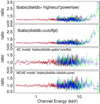 |
Fig. 1. Data-to-model ratio vs. energy plot for the phase-averaged broadband (XMM-Newton plus NuSTAR) spectrum of NGC 300 ULX1. Top two panels: absorbed power-law models with exponential roll-off (using two different Xspec models). Two lower panels: AC and MCAE models, respectively. |
Central values and confidence levels based on the marginalized parameter distribution of the Bayesian model comparison for the broadband fit of combined XMM-Newton and NuSTAR observation of NGC300 ULX-1 for phase-averaged (FULL) and phase-resolved spectra (ON- and OFF-pulse).
MCAE model. We fit the spectral continuum with the MCAE combination of two MCD components and a power-law high-energy tail. Interstellar absorption was treated similarly to the AC model. The dual thermal model yields a fit with reduced χ2 value of 1.09 for 764 d.o.f., which is an improvement of Δχ2 of 95 to the AC model. The bottom panel of Fig. 1 presents the data-to-model ratio, where no prominent residuals are apparent. We note that the MCAE model for the spectral continuum has six free parameters and the AC model has five free parameters.
3.4. Phase-resolved spectroscopy
We followed Carpano et al. (2018) to derive the pulse profile of the neutron star (Fig. 3). To search for spectral changes with spin phase, we studied the phase-resolved hardness ratio (HR). We define HR as HRi = (Ri + 1 − Ri)/(Ri + 1 + Ri), with Ri and Ri + 1 denoting the background-subtracted count rates in two consecutive energy bands. For the XMM-Newton/EPIC-pn detector, we used three energy bands (0.3–2.0 keV, 2.0–4.5 keV, and 4.5–10.0 keV), while for NuSTAR, we used two energy bands (3.0–10.0 keV and 10.0–20.0 keV). Thus we defined three distinct HRs as shown in Fig. 3. From this first exercise, it is clear that only the softer HR varies with phase. Specifically, we see that HR1 becomes softer when fainter. This behavior is characteristic of the soft excess seen in XRPs (e.g., Klochkov et al. 2011; Postnov et al. 2015; Koliopanos & Vasilopoulos 2018).
Using the temporal information obtained from the source light curve, we extracted phase-resolved spectra during the peak (ON-pulse) and the trough of the pulse profile (OFF-pulse), see Fig. 3. We studied the phase-resolved spectra by fitting them in a similar way as previously for the phase-averaged spectra. The broadband ON- and OFF-pulse spectra were fit separately using the same models as in the phase-averaged spectrum. We monitored the behavior of the spectral components and the absorption, and the variation of their best-fit parameters with phase. The resulting best-fit values (i.e., the median value of the posterior distribution and 90% error bars) for the spectral modeling are presented in Table 1. For purposes of presentation and to note the relative persistence of the soft emission versus the variability of the harder emission, we also simultaneously unfolded the ON- and OFF-pulse spectra from a model frozen in the best-fit parameters of the phase-averaged (FULL) MCAE fit. In Fig. 4 we present the unfolded spectra and data-to-model ratio versus energy plots to provide a qualitative assessment of this behavior.
3.5. Possible broad absorption line residuals
When we increased the Efold value in the cutoffpl model in order to account for the high-energy (> 15 keV) positive residuals, we noted broad negative residuals between ∼8 and ∼20 keV (see Fig. 5). Given the presence of a highly magnetized neutron star accretor, the broad absorption feature can be interpreted as a potential cyclotron resonant scattering feature (CRSF, e.g., Heindl et al. 2004). Modeling the broad absorption-like feature with a Gaussian absorption line (Xspec model gabs) improves the quality of the AC model fit by a Δχ2 of 110 for three d.o.f. As the third panel from the top of Fig. 1 shows, the high-energy continuum is now adequately described. The absorption line is centered at ∼13.1 keV and has a width of ∼3.7 keV (see Table 1, AC model, “Full”).
Although a visual inspection of the residuals from the MCAE model does not reveal a need for an additional absorption feature (Fig. 1, bottom panel), adding a Gaussian absorption line introduces a moderate improvement to the model (Δχ2 of 12 for 3 d.o.f.), indicating the detection of a broad absorption line that is constrained at values (Egabs ∼ 12 keV and width of ∼3 keV) similar to those of the AC model fit. However, there is considerable degeneracy between line parameters and the parameters of the hot MCD and the power-law tail. For a region of parameter space the absorption line does not seem to be required by the MCAE fit.
A problem of comparison between two different but physically motivated models emerges in the effort of determining whether the broad absorption-like feature can be incorporated in our modeling. A simple comparison between χ2 values cannot fully explore the multidimensional parameter space that needs to be investigated in order to attain satisfactory constraints on the absorption feature. To pursue this task, we employed a Bayesian model selection framework.
4. Bayesian X-ray analysis
4.1. Overview of Bayesian method
To compare the two competing models, AC and MCAE, we used a Bayesian methodology (see Buchner et al. 2014). The evidence Z is defined as
![Mathematical equation: $$ \begin{aligned} Z=\int \,\pi (\boldsymbol{\theta })\,\exp \left[-\chi ^2(\boldsymbol{\theta })/2\right]\, \mathrm{d}\boldsymbol{\theta }, \end{aligned} $$](/articles/aa/full_html/2019/01/aa34144-18/aa34144-18-eq69.gif)
where θ is the parameter vector of the model, χ2 is the fit statistic, and π(θ) dθ is the metric of the parameter space, which weights the various regions (prior). In this work, we use uninformative priors throughout.
While commonly used model comparison methods include likelihood ratios at the best-fit or information criteria, here we prefer the model with the highest Z: the ratio of Z values from two models, the Bayes factor, can be used to assess their suitability. Intuitively speaking, log Z indicates the quality of the fit (i.e., −χ2/2) minus a penalty for size of the model parameter space. In Bayesian model selection, prediction diversity distant from the observed data is punished. The Bayesian approach is appealing because it does not assume the true value to be equal to the best fit and takes into account the uncertainties and the model complexity. While priors need to be specified on all parameters, primarily the priors on parameters that are different between models are influential.
To compute the evidence Z, we used the Bayesian X-ray analysis package (BXA). The BXA package5 (Buchner et al. 2014) connects the nested sampling (Skilling 2004) algorithm MultiNest (Feroz et al. 2009) with Xspec. It explores the parameter space and can be used for parameter estimation (probability distributions of each model parameter and their degeneracies) and model comparison (computation of Z). We used BXA with its default parameters (400 live points and log Z accuracy of 0.1). With this Bayesian framework, we are able to test and compare the physically motivated spectral models described above with the X-ray spectrum of NGC 300 ULX1. Moreover, we are able to test the variability of the spectral components with the spin pulse-phase.
4.2. BXA results for NGC 300 ULX1
We ran the BXA routine for the entire set of models and for the phase-averaged and resolved spectra, presented in Sect. 3. We present the resulting log Z values in Table 2.
Our analysis confirms that the AC model with a Gaussian absorption line is preferable to the one without, as both phase-averaged and resolved spectra have a significantly higher Z value when modeled with the AC model that includes the feature. However, we further find that both the MCAE models with and without the line provide a better fit to the data, with the MCAE model without the line providing the superior fit to the phase-averaged (“Full”) data set of all models considered. The “Full (no line)” MCAE fit (see Table 1) yields a log Z value of ∼ − 460.6 and with a Δlog Z of ∼6.4 from the AC model with the Gaussian absorption line and a Δlog Z of ∼1.0 from the MCAE model with the line, it is the significantly preferable model. Based on the global evidence, the MCAE model with the Gaussian absorption line is about 25 times less likely than the simple MCAE fit. The same results are generated for the “ON-pulse” and “OFF-pulse” spectra as well (see Table 2). In the following we focus on the analysis of the phase-averaged spectra as they have the best statistics, allowing for the significant detection of the absorption-like feature in the “AC model”. In Table 2 we tabulate the log Z values of the two continuum models with or without the absorption feature for the phase-averaged data set (which has the best statistics to constrain the presence or absence of the line) and the log Z values of the two continuum models with the absorption line for the ON- and OFF-pulse data sets. Finally, we used the BXA to also compare between the cutoffpl and the powerlaw*highecut models. The algorithm confirms that the presence of the Gaussian absorption line is also preferred in the powerlaw*highecut model. There is no significant difference in the preference between the two models, although it appears that without the absorption feature the powerlaw*highecut model yields a marginally better log Z value, but when including the Gaussian absorption feature, the cutoffpl (AC model) is preferable. In all cases, the MCAE model without the absorption line is the preferred model (see Table A.1). We note that we compared models with a different number of free parameters (e.g., the AC model with the Gaussian absorption has two additional free parameters with respect to the MCAE model, which does not require it). Nevertheless, the Bayesian model comparison punishes the increase in prediction diversity that is caused by any additional free parameter(s). Therefore, the BXA is a more reliable method for model comparison and can more efficiently identify irrelevant parameters. For a more detailed discussion of this point, we refer to (e.g., Sect. 2.4 of Baronchelli et al. 2018).
Closer exploration of the parameter space of the MCAE fit revealed a well-defined region for which the emission line becomes undetectable. The region is defined by lower temperatures for the hot thermal component (i.e., kThot ≲ 2.4 keV, see Fig. 6, left panel) combined with low values of the power-law spectral index (see Fig. 6, right panel), in agreement with the values expected for ULXs within the MCAE paradigm (Mushtukov et al. 2017; Koliopanos et al. 2017). We also note that the tabulated values in Table 1 are not the best-fit values of a single spectral fitting, but the posterior distribution of each model parameter in the 90% confidence range. The central values are the median of the distribution. It is important to stress that while in a Gaussian distribution the median would coincide with the most likely value of the parameter, this is not the case here, especially in the MCAE model.
In our scheme the hot MCD model is used as a rough approximation of the multi-temperature thermal emission of a spheroidal accretion envelope, therefore the size of the value of the inner radius that corresponds to the tabulated value of Kdisk is physically meaningless (see the discussion in Koliopanos et al. 2017). Alternatively, we can also model the envelope emission with a spherical blackbody model (Xspec model bbodyrad). This model yields a radius of  km for a temperature of 1.56 ± 0.03 keV (see Table A.2). The bbodyrad fit returns a reduced χ2 of 1.11 (a Δχ2 increase of 8 for the same d.o.f. as the diskbb fit). The increase may be an indication that the hot thermal emission is indeed better described by a multi-temperature thermal component than by a simple blackbody. However, the χ2 of the bbodyrad fit is within an acceptable range, and further comparison between the two components is beyond our scope. The bbodyrad fit is only used to provide a rough estimate of the size of the emitting region, using a more physical parameter (i.e., the size of a thermally emitting sphere). The best-fit values and the MCAE fit using both the diskbb and bbodyrad models are tabulated in Table A.2 in the appendix (we recall that the main Table 1 presents the central values and confidence levels of the model parameters from the BXA analysis).
5. Discussion
Modeling the broadband emission of NGC 300 ULX1 reveals a spectrum that shares similarities with the spectra of accreting XRPs and ULXs. The spectral continuum is comprised of two distinct components: A soft thermal-like excess, and a hard power-law like component with a high-energy roll-over. We find that the presence of considerable residual structure in the high-energy (> 8 keV) spectral continuum of the source can be modeled using a broad Gaussian absorption feature that can be interpreted as a CRSF. If confirmed by further observations, this is the first cyclotron-scattering feature detected in an accretion-powered pulsar at this luminosity regime and can have profound implications on our understanding of the super-Eddington accretion onto high-B neutron stars and ULXs in general. However, we also find that when the spectral continuum is modeled using recent models for the spectra of pulsating ULXs (Mushtukov et al. 2017; Koliopanos et al. 2017), the absorption feature is not required. Below we discuss the two models we used to fit the spectral continuum of NGC 300 ULX1, present the different emission components we identified in the source spectrum, and investigate their significance and behavior with pulse phase.
5.1. Soft thermal component
In all our spectral fits we significantly detect a soft thermal component, which can be described well by a ∼0.3 keV multicolor disk with an inner radius between 400 and 800 km (see Table 1 for the MCAE and AC models and assuming an inclination angle of 60°). The characteristics of the soft thermal component are consistent with a geometrically thin accretion disk truncated at the magnetosphere of a dipole magnetic field with an equatorial strength of ∼3 − 7 × 10¹² G, assuming the expressions in Lai (2014; see also Eq. (1) from Mushtukov et al. 2017). We note that this is only a rough estimate that suggests a magnetic field strength that is higher than 1012 G. Different disk inclinations (e.g., a few degrees inclination, as is suggested from the upper limit in the orbital plane in Carpano et al. 2018) can affect the B-value by a factor of ∼2 if we further take into account the color correction expected for the spectral emission of a disk of > 200 eV temperature (see London et al. 1986; Lapidus et al. 1986; Shimura & Takahara 1995 and Sect. 3 in Koliopanos et al. 2017), we expect an increase of a factor of more than six in the B-value, thus exceeding 1013 G.
The column density and the emission intensity vary over the pulse phase. They appear to be positively correlated and peak during the ON-pulse phase. This can be seen in the LX and NH panels in Fig. A.1 (first panel) and Fig. A.2 for the AC and MCAE fits, respectively. The correlation is more pronounced in the AC model. However, we must note that there is considerable degeneracy between the soft thermal emission, the value of NH, and the tail of the pulsating, hard component. In the AC model, the nonthermal emission of the accretion column should also feature a low-energy roll-over, characteristic of the thermal or Bremsstrahlung seed photons that generate it. However, no such component is included in any of the simple power-law models we considered. As the flux of the nonthermal component varies with pulse phase (see discussion below), this will also affect the low-energy part of the spectrum. The variability of the soft thermal component and of NH is most likely due to this effect, rather than an inherent source characteristic (see also the discussion in Koliopanos & Vasilopoulos 2018). This problem is less pronounced in the MCAE model, since the diskbb model, used to fit the hot thermal emission of the accretion envelope, exhibits the Rayleigh–Jeans tail at low energies.
5.2. Accretion column model
The high-energy part of the source continuum was modeled using a hard power-law with a spectral index of ∼0.7 and Efold of ∼6 keV (with the addition of Gaussian absorption line, see Table 1, AC model “Full”, and Sect. 5.3 below). This spectrum is qualitatively similar to the spectra expected for the emission of the accretion column in highly magnetized neutron stars (e.g., White et al. 1983; Becker & Wolff 2007). However, the energy of the cutoff is detected at an unusually low energy (Ecut ≈ 6 keV, see Sect. 3.1 and also Carpano et al. 2018) compared to Ecut ∼ 20 − 30 keV observed in most nominal X-ray pulsars (e.g., White et al. 1983; Di Salvo et al. 1998; Coburn et al. 2002; Miyasaka et al. 2013; Fürst et al. 2013, 2014; Fornasini et al. 2017) and also predicted by thermal and bulk Comptonization models in the accretion column (e.g., Becker & Wolff 2007). On the other hand, the observed roll-off energy of NGC 300 ULX1 is similar to that of most ULXs (e.g., Stobbart et al. 2006; Roberts 2007; Gladstone et al. 2009; Sutton et al. 2013).
The absolute flux of the cPL component clearly changes with pulse phase, with a value of 10.5 ± 0.2 × 10⁻¹² erg cm−2 s−1 during ON-pulse and 1.7 ± 0.1 × 10⁻¹² erg cm−2 s−1 during OFF-pulse. This behavior is also shown by the flux ratio between the soft thermal component and the cutoff power-law, which is FcPL/Fdisk = 7.3 ± 0.5 during ON-pulse and FcPL/Fdisk = 2.2 ± 0.8 during OFF-pulse (see also Fig. 4). This correlation indicates that the nonthermal emission is the source of the pulsations. It can therefore be argued that the power-law component originates in the accretion column of a high-B neutron star.
The nonthermal emission in X-ray pulsars often exhibits an anticorrelation with the pulse amplitude, such that the continuum or power law becomes harder near the pulse peak (e.g., Klochkov et al. 2011; Malacaria et al. 2015; Vybornov et al. 2017; Koliopanos & Vasilopoulos 2018). In the context of an accretion column, the hardening of the slope can be understood in terms of change in the inclination angle at which the observer views the column during ON- and OFF-pulse. Assuming that the accretion column is viewed closer to the face-on orientation during the ON-Pulse phase, it is also reasonable to assume that the scattering optical depth will increase, resulting in a harder slope. This can be understood in terms of the Comptonization y-parameter and the scattering of low-energy photons at high optical depths tha tis expected in the accretion column: Comptonized photons with hν ≪ kTe are expected to follow a power-law distribution with F(E)=C E−Γ, where E is the photon energy (e.g., Pozdnyakov et al. 1983), where  (e.g., Rybicki & Lightman 1979), and y is the Comptonization y-parameter, which in the presence of a strong magnetic field and high optical depth is given by y = 2/15 (kT/mec2)τ2 (Basko & Sunyaev 1975). Therefore, as the optical depth increases, the power-law emission is expected to become harder.
This behavior is not observed in NGC 300 ULX1. The median fitted power-law slope in the ON-phase is higher than the OFF-phase, within their fairly high 90% error bars. According to Table 1 and Fig. A.1, the two values are consistent with each other, but also allow a change in Γ by ∼0.3 between ON- and OFF-phase. The uncertainty in the value of the spectral index is partially due to degeneracy between the index, the cutoff energy, and the cross-calibration parameters between the detectors of the two telescopes. When the cross-calibration parameters are frozen, the BXA yields a value of Γ = 0.63 ± 0.10 for the ON-pulse spectrum and Γ = 0.68 ± 0.15 for the OFF-pulse spectrum. The absence of pulse-correlated hardening is further visible in the 3–10 keV/10–20 keV hardness ratio versus pulse phase in Fig. 3.
5.3. Possible cyclotron line
The smooth AC model cannot adequately fit the > 10 keV range of the emission unless a broadened absorption line is added (see Fig. 1). In the context of a highly magnetized neutron star, this feature can be interpreted as electron cyclotron scattering. The broad and shallow absorption feature in NGC 300 ULX1 differs from the recently suggested narrow and deep feature in M51 ULX-8, which favors a proton cyclotron line (Brightman et al. 2018). The identification of the line centroid energy is a robust method to estimate the magnetic field strength of the scattering region in an neutron star. The approximate relation between the observed electron cyclotron energy and the magnetic field strength in the scattering region is given by
 (3)
(3)
where B12 is the magnetic field in units of 1012 G and z ∼ 0.15 is the gravitational redshift for standard neutron star parameters. If the presence of the cyclotron line is true, a line centroid at ∼13 keV implies a magnetic field strength of B ∼ 1012 G. However, this magnetic field estimate may not reflect the surface magnetic field strength of the neutron star as the accretion column (and hence the line-forming region) of an ULX may be formed several kilometers above the surface, depending on the mass accretion rate and the surface magnetic field strength (Mushtukov et al. 2015). Furthermore, magnetar-like field strengths are expected for ULXs as the average electron scattering cross-section is significantly reduced at high enough magnetic field strengths, implying higher peak luminosities. Therefore the maximum accretion luminosity can be used to constrain the surface field strength of the neutron star as  (Mushtukov et al. 2014). In the case of NGC 300 ULX1, a peak luminosity of 4.5×1039 erg s−1 (0.3–30 keV) implies a surface magnetic field strength of ≳2 × 10¹³ G.
While this value is inconsistent with the centroid energy of the line, it is in agreement with estimates from accretion torque theory, based on the observed source spin-up rate (Vasilopoulos et al. 2018). Assuming a dipolar magnetic field, the difference between the estimated field strength and the strength, derived from absorption features, imply a very tall accretion column of height ∼1.7RNS. However, the dependence of the line on the continuum modeling makes it highly uncertain, and this needs to be confirmed by future deeper observations.
Recent theoretical considerations argue that the cyclotron line may form when the radiation emitted by the accretion column is reflected off the neutron star surface (Poutanen et al. 2013). As the accretion rate increases, the accretion column grows larger, as does the illuminated fraction of the stellar surface, which weakens the average magnetic field and reduces the cyclotron line energy. If the accretion rate continues to increase (as the source luminosity persistently exceeds the Eddington limit), the height of the column will also increase, gradually reducing the fraction of its emission reflected of the neutron star surface. As a result, in the cyclotron reflection paradigm, very luminous sources will be expected to feature very weak cyclotron lines. The saturation of the reflected component is observationally indicated at LX ∼ 1038 erg s−1 (e.g., Postnov et al. 2015), above which the height of the accretion column is expected to exceed multiple times the radius of the neutron star and thus the reflected fraction is expected to become insignificant (e.g., Fig. 2 Poutanen et al. 2013).
The presence of a possible cyclotron line in NGC 300 ULX1 was first reported by Walton et al. (2018a). Walton et al. (2018a) presented the detection of the absorption-like feature, assuming the underlying continuum comprised of a cutoff power law and a soft thermal component. The authors interpreted the feature as a CRSF and then focused their discussion on the important consequences of this discovery. With a more thorough and refined statistical analysis, we confirm the findings of Walton et al. (2018a) under assumptions similar to theirs, but we also explore the possibility that the presence of this broad absorption-like feature is contingent upon the choice of the underlying model. This caveat is acutely important since the alternative model (i.e., the MCAE model discussed below) is a physically motivated model, its best-fit parameter values are consistent with the values found for other ULXs (e.g., Koliopanos et al. 2017; Walton et al. 2018b), and it does not require the addition of an absorption line.
5.4. Multicolor accretion envelope model
As the source luminosity lies well within the range of ULXs, we also modeled the spectrum using the MCAE model, based on the predictions of Mushtukov et al. (2017) and following the modeling scheme presented in Koliopanos et al. (2017). The continuum is described by two MCDs and a faint power-law tail. This model is similar to the one used for ULXs in Koliopanos et al. (2017), and the best-fit values lie within the range found in that work. In the context of the MCAE model, the soft MCD component originates in the truncated disk, similar to the AC model, while the hot MCD component is interpreted as emission from an optically thick accretion envelope that is predicted to engulf the entire neutron star and almost entirely reprocesses the emission of the accretion column (see Mushtukov et al. 2017, and Sect. 3.2).
The hot thermal component naturally explains the unusually low energy of the spectral roll-off and can potentially reproduce the smooth, single-peaked pulsations, which in the context of the MCAE are the result of an extended, rotating, hot, optically thick emitting region that heavily distorts the original pulse-profile of the accretion column (Mushtukov et al. 2017). Finally, the presence of a fainter, hard power-law tail is similar to those detected in all ULXs with available NuSTAR spectra in Koliopanos et al. (2017). More importantly, the MCAE fit does not require the presence of the Gaussian absorption line.
The analysis with BXA revealed two different parameter solutions for the MCAE model that can be easily shown in Figs. 6 and A.4. In one solution (presented in Table 1), the broad absorption-like feature can be detected, moderately increasing the log Z value, while in the second solution, it is not detected (see Fig. A.4). The model comparison using the log Z value favors the MCAE model (with or without the Gaussian absorption line) over the AC model (with the inclusion of the line). Furthermore, the preferred solution out of all models is the MCAE model without the Gaussian absorption line. This finding casts legitimate doubts on the robustness of a CRSF discovery.
We note that in this model, which is based on fundamental principles, at the mass accretion rate implied by the observed luminosity, the accretion shell becomes partially or fully optically thick (see Eq. (2) and Fig. 2). In addition to the shape of the pulse profile, the presence of an optically thick accretion envelope would also explain the fact that the pulsed component does not become harder during the ON-pulse phase. In this scenario, pulsations naturally arise from the rotation of the accretion funnel as the observing angle of its surface would change with pulse phase. This is in contrast to the explanation given by Walton et al. (2018a), where the authors in general attributed the diluted pulsed profiles of PULXs to the presence of quadrupolar magnetic field geometry. Given the dimensions of the accretion column and the optical thick funnel or envelope around it, this contradicts their assumption that emission originates from near the neutron star surface. Both features are more consistent with emission from a hot region on a rotating area than with anisotropic nonthermal emission from an accretion column. Therefore, the presence of a dual thermal spectrum is a likely scenario and the use of the MCAE model is physically motivated.
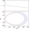 |
Fig. 2. Structure of the accretion envelope. Optical depth at a distance. Across the envelope, the optical depth has been computed based on the minimum separation of the two confining lines. The separation of the lines (i.e., the base of the accretion column) has been selected to be 100 m (see discussion in West et al. 2017). |
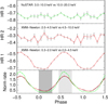 |
Fig. 3. Bottom panel: pulse profile of NGC 300 ULX1, using the 2016 XMM-Newton/EPIC-pn (black, and red lines; 0.3–10.0 keV) and NuSTAR data (green lines; 3.0–30.0 keV). ON-pulse and OFF-pulse spectra were extracted from the gray shaded areas, which have a width of 0.3 in phase. Top panels: XMM-Newton HR1: 0.3-2.0 vs. 2.0-4.5, HR2: 2.0–4.5 vs. 4.5–10.0, and NuSTAR HR3: 3.0–10.0 vs. 10.0–20.0. |
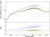 |
Fig. 4. Unfolded spectra and data-to-model ratio plot of the ON-pulse, OFF-pulse, and FULL (phase-averaged) spectra from the MCAE modeling of the phase-averaged emission. |
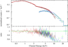 |
Fig. 5. Phase-averaged broadband (XMM-Newton plus NuSTAR) X-ray spectrum of NGC 300 ULX1 (upper panel) plotted together with the data-to-model ratio for the absorbed AC model (lower panel). For illustration purposes the strength of the absorption line has been set to zero. |
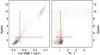 |
Fig. 6. Marginalized parameters of the line depth (Kgabs, see Table 1 for details), temperature of the hot thermal component, and slope of power-law tail for the MCAE model. The red lines mark the 5%, 50% (cross-section) and 95% percentiles of the 1D distributions. For the distributions of Fig. A.1 we have plotted the 2D histograms for the two pairs of parameters (for the full parameter space, see Fig. A.4). |
Since the inner disk radius provided by the MCD model, which we used to fit the hot thermal emission, lacks a physical meaning in the context of a spheroidal envelope, we consider the value of the spherical black body (BB) fit presented in Sect. 3. The BB model yields a size of RBB = 50 ± 11 km. As a simple spherical blackbody is a simplification of the predicted multicolor emission of the accretion envelope, this estimate can be viewed only as indicative of the size of the emitting region, which lies in the ∼100 km range. The estimated size is smaller than the size of the magnetosphere, inferred from the soft MCD component (see Fig. A.2 panel 2, top row), and since most of the hot thermal emission originates from the hottest region of the accretion envelope, we can assume that RBB is the size of this extended emission region, which occupies only a fraction of the optically thick accretion envelope. Last, considering the uncertainty in the source inclination, we can reasonably argue that the value of RBB and the inner disk radius are in rough agreement. If we further assume that the CRSF can be detected in the accretion envelope paradigm, and assuming that it is formed at a distance of 50 km from the neutron star surface, we infer a magnetic field strength of 5 − 6 × 10¹³ G on the surface of the neutron star.
This is in rough agreement with the luminosity-based estimate and the estimate from accretion torque theory (Vasilopoulos et al. 2018). However, we must stress that (particularly) within the paradigm that posits that the cyclotron line is formed as a result of neutron star surface reflection (Poutanen et al. 2013) and for the MCAE model, the (weak) line would most likely not be detected due to obscuration of the central source. This would explain why within this framework a cyclotron line is indeed not significantly detected.
5.5. Physical interpretation of fit derived quantities
Measurement of the size of the emitting region can also provide a consistency or validity check between the AC and MCAE models. The fundamental difference of the two models is that the AC model predicts nonthermal (cPL) emission from the accretion column as the source of the pulsations, while the MCAE predicts hot thermal emission from an optically thick envelope. In both cases a characteristic effective temperature Teff can be derived by the observed LX, assuming a size for the emitting region (i.e.,  ). Moreover, 3 kTeff ≲ Ecut, and thus the size of the emitting region should be larger than
  , which yields a value of > 50 km for the cutoff energy of the observed spectrum (Ecut ∼ 6, see Sect. 3.1 and also Carpano et al. 2018). The luminosity-derived size and the spectral-fit-derived size of RBB ∼ 50 km are unphysically high for an accretion column (Mushtukov et al. 2015), thus challenging the basic principles of the AC model. In contrast, these sizes are in good agreement with the inner part of the magnetospheric envelope with the highest optical depth (see Fig. 2).
Last, we note that the existence of the two areas (with and without the absorption feature) in the MCAE parameter space as revealed by the BXA runs (e.g., row 3, Col. 4, Fig. A.2) signifies that the redundancy of the cyclotron-like feature may not be limited to the MCAE model alone, but a set of models with a more complex continuum. It appears that the cyclotron feature is required by the model for a high kThot, resembling the smooth continuum of the AC model. The BXA results suggest that there are two classes of solutions to the problem of the ∼10 keV residual structure: A smooth continuum that requires a broad absorption-like feature, or a more complex continuum comprised of more than one component for the high-energy part.
In our analysis we explored the MCAE model. However, a more complex spectral continuum is also predicted for the broadband emission of the accretion column, as a result of bulk and thermal Comptonization of thermal and Bremsstrahlung photons (e.g., Becker & Wolff 2007; Farinelli et al. 2012, 2016). As these models consider the accretion column emission in X-ray pulsars below the ULX luminosity, they do not take into account the optically thick structure that is expected to form around the accretion column and in the surrounding magnetosphere. For this reason, we considered the MCAE model as an alternative to a smooth cutoff power-law continuum. The MCAE model is a better description of the data according to the Bayesian model comparison.
6. Conclusions
We have carried out phase-resolved, broadband spectroscopy of NGC 300 ULX1. Our analysis reveals an accretion disk, indicated by non-pulsating soft thermal emission. This is consistent with a disk truncated at approximately the magnetospheric radius of a highly magnetised neutron star. We further find that an additional hard emission component is responsible for the observed pulsations. The flux of this component strongly varies with the pulse phase, but not significantly with its spectral hardness.
We find indications for a broad absorption-like feature that in the context of a highly magnetized neutron star may be interpreted as an electron cyclotron line. If it is real, this would be the first such feature detected in an pulsating ULX, providing some constraint on the B-field of such a source. However, we find a strong dependence between the line and the choice of the underlying continuum model. To further probe this dependence, we considered two different models for the source continuum, the AC and MCAE. If the source continuum is modeled using the recently suggested MCAE model (Mushtukov et al. 2017; Koliopanos et al. 2017) for the spectra of (pulsating) ULXs, an absorption line is not required in order to successfully model the source spectrum. Therefore, the cyclotron line must be considered with great caution.
To further probe the suitability of each of the two models, we employed Bayesian techniques for model comparison and also qualitatively evaluated the physical characteristics of the source as inferred from the two models. The Bayesian analysis demonstrated that the MCAE model is preferable to the AC model and that while the cyclotron line in case of the MCAE model cannot be ruled out, there is a well-defined region in the MCAE parameter space within which the cyclotron line is not detected. Furthermore, the Bayesian model comparisons suggest that in the context of the MCAE, the model without the line is more likely than the one that includes it. The cyclotron line is detected with much higher significance in the context of the AC model, which is observed in most XRPs. However, if the observed emission originates in an accretion column, questions arise with respect to the very low energy of the roll-off, the shape of the pulse profile, the relation between the spectral slope and the pulse phase, and the inferred size of the emitting region.
All these source characteristics can be better understood in the context of the MCAE model, within which a cyclotron line is less probable. A third possibility involves the existence of the CRSF in the MCAE framework, in which case the inferred magnetic field strength on the surface of the neutron star is estimated to be higher than 1013 G. However, this a value would be quite surprising in this context because of the obscuring effects of the accretion envelope, but also in the AC model context if the origin of the cyclotron emission is due to reflection off the neutron star surface.
Confirmation of the cyclotron feature in NGC 300 ULX1 is of great importance, as it will not only provide an indication of the magnetic field strength, but also provide crucial insight into the shape of the underlying continuum, which is still a matter of considerable debate for the ULX population. Therefore, deeper NuSTAR observations of the source are strongly encouraged.
We define the S/N based on the total number of source (Nsrc) and background (Nbg) events that are collected from areas with the same size as: ( ).
).
The photon distribution is ∝E−Γexp−E/β, where Γ is the photon index and β the e-folding energy of the exponential roll-off.
BXA is available at https://github.com/JohannesBuchner/BXA
Acknowledgments
The authors would like to thank the anonymous referee, whose contribution significantly improved our manuscript. FK acknowledges support from the CNES. JB acknowledges support from the CONICYT-Chile grants Basal-CATA PFB-06/2007, FONDECYT Postdoctorados 3160439, and the Ministry of Economy, Development, and Tourism’s Millennium Science Initiative through grant IC120009, awarded to The Millennium Institute of Astrophysics, MAS.
References
- Arnaud, K. A. 1996, in Astronomical Data Analysis Software and Systems V, eds. G. H. Jacoby, & J. Barnes, ASP Conf. Ser., 101, 17 [Google Scholar]
- Bachetti, M., Harrison, F. A., Walton, D. J., et al. 2014, Nature, 514, 202 [NASA ADS] [CrossRef] [Google Scholar]
- Balucinska-Church, M., & McCammon, D. 1992, ApJ, 400, 699 [NASA ADS] [CrossRef] [Google Scholar]
- Baronchelli, L., Nandra, K., & Buchner, J. 2018, MNRAS, 480, 2377 [NASA ADS] [Google Scholar]
- Basko, M. M., & Sunyaev, R. A. 1975, A&A, 42, 311 [NASA ADS] [Google Scholar]
- Basko, M. M., & Sunyaev, R. A. 1976, MNRAS, 175, 395 [NASA ADS] [CrossRef] [Google Scholar]
- Becker, P. A., & Wolff, M. T. 2007, ApJ, 654, 435 [NASA ADS] [CrossRef] [Google Scholar]
- Binder, B., Williams, B. F., Kong, A. K. H., et al. 2011, ApJ, 739, L51 [NASA ADS] [CrossRef] [Google Scholar]
- Brightman, M., Baloković, M., Koss, M., et al. 2018, ApJ, 867, 110 [NASA ADS] [CrossRef] [Google Scholar]
- Buchner, J., Georgakakis, A., Nandra, K., et al. 2014, A&A, 564, A125 [NASA ADS] [CrossRef] [EDP Sciences] [Google Scholar]
- Burnard, D. J., Arons, J., & Klein, R. I. 1991, ApJ, 367, 575 [CrossRef] [Google Scholar]
- Carpano, S., Haberl, F., Maitra, C., & Vasilopoulos, G. 2018, MNRAS, 476, L45 [NASA ADS] [CrossRef] [Google Scholar]
- Cash, W. 1979, ApJ, 228, 939 [NASA ADS] [CrossRef] [Google Scholar]
- Chashkina, A., Abolmasov, P., & Poutanen, J. 2017, MNRAS, 470, 2799 [NASA ADS] [CrossRef] [Google Scholar]
- Coburn, W., Heindl, W. A., Rothschild, R. E., et al. 2002, ApJ, 580, 394 [NASA ADS] [CrossRef] [Google Scholar]
- Colbert, E. J. M., & Mushotzky, R. F. 1999, ApJ, 519, 89 [NASA ADS] [CrossRef] [Google Scholar]
- Di Salvo, T., Burderi, L., Robba, N. R., & Guainazzi, M. 1998, ApJ, 509, 897 [NASA ADS] [CrossRef] [Google Scholar]
- Farinelli, R., Romano, P., Mangano, V., et al. 2012, MNRAS, 424, 2854 [NASA ADS] [CrossRef] [Google Scholar]
- Farinelli, R., Ferrigno, C., Bozzo, E., & Becker, P. A. 2016, A&A, 591, A29 [NASA ADS] [CrossRef] [EDP Sciences] [Google Scholar]
- Feroz, F., Hobson, M. P., & Bridges, M. 2009, MNRAS, 398, 1601 [NASA ADS] [CrossRef] [Google Scholar]
- Fornasini, F. M., Tomsick, J. A., Bachetti, M., et al. 2017, ApJ, 841, 35 [NASA ADS] [CrossRef] [Google Scholar]
- Fürst, F., Grefenstette, B. W., Staubert, R., et al. 2013, ApJ, 779, 69 [NASA ADS] [CrossRef] [Google Scholar]
- Fürst, F., Pottschmidt, K., Wilms, J., et al. 2014, ApJ, 780, 133 [NASA ADS] [CrossRef] [Google Scholar]
- Fürst, F., Walton, D. J., Harrison, F. A., et al. 2016, ApJ, 831, L14 [NASA ADS] [CrossRef] [Google Scholar]
- Gao, Y., Wang, Q. D., Appleton, P. N., & Lucas, R. A. 2003, ApJ, 596, L171 [NASA ADS] [CrossRef] [Google Scholar]
- Gilfanov, M., Grimm, H.-J., & Sunyaev, R. 2004, Nucl. Phys. B Proc. Suppl., 132, 369 [NASA ADS] [CrossRef] [Google Scholar]
- Gladstone, J. C., Roberts, T. P., & Done, C. 2009, MNRAS, 397, 1836 [NASA ADS] [CrossRef] [Google Scholar]
- Heindl, W. A., Rothschild, R. E., Coburn, W., et al. 2004, in X-ray Timing 2003: Rossiand Beyond, eds. P. Kaaret, F. K. Lamb, & J. H. Swank, Am. Inst. Phys. Conf. Ser., 714, 323 [Google Scholar]
- Hickox, R. C., Narayan, R., & Kallman, T. R. 2004, ApJ, 614, 881 [NASA ADS] [CrossRef] [Google Scholar]
- Israel, G. L., Belfiore, A., Stella, L., et al. 2017a, Science, 355, 817 [NASA ADS] [CrossRef] [Google Scholar]
- Israel, G. L., Papitto, A., Esposito, P., et al. 2017b, MNRAS, 466, L48 [NASA ADS] [CrossRef] [Google Scholar]
- Kaaret, P., Prestwich, A. H., Zezas, A., et al. 2001, MNRAS, 321, L29 [Google Scholar]
- Kaminker, A. D., Fedorenko, V. N., & Tsygan, A. I. 1976, Sov. Astron., 20, 436 [NASA ADS] [Google Scholar]
- King, A., Lasota, J.-P., & Kluźniak, W. 2017, MNRAS, 468, L59 [NASA ADS] [CrossRef] [Google Scholar]
- King, A. R. 2009, MNRAS, 393, L41 [NASA ADS] [Google Scholar]
- Klochkov, D., Staubert, R., Santangelo, A., Rothschild, R. E., & Ferrigno, C. 2011, A&A, 532, A126 [NASA ADS] [CrossRef] [EDP Sciences] [Google Scholar]
- Koliopanos, F. 2017, Proceedings of the XII Multifrequency Behaviour of High Energy Cosmic Sources Workshop. 12–17 June, 2017 Palermo, Italy (MULTIF2017), Online at https://pos.sissa.it/cgi-bin/reader/conf.cgi?confid=306, 51 [Google Scholar]
- Koliopanos, F., & Vasilopoulos, G. 2018, A&A, 614, A23 [NASA ADS] [EDP Sciences] [Google Scholar]
- Koliopanos, F., Vasilopoulos, G., Godet, O., et al. 2017, A&A, 608, A47 [NASA ADS] [CrossRef] [EDP Sciences] [Google Scholar]
- Kosec, P., Pinto, C., Fabian, A. C., & Walton, D. J. 2018a, MNRAS, 473, 5680 [NASA ADS] [CrossRef] [Google Scholar]
- Kosec, P., Pinto, C., Walton, D. J., et al. 2018b, MNRAS, 479, 3978 [NASA ADS] [Google Scholar]
- Lai, D. 2014, Eur. Phys. J. Web Conf., 64, 01001 [Google Scholar]
- Lapidus, I. I., Syunyaev, R. A., & Titarchuk, L. G. 1986, Sov. Astron. Lett., 12, 383 [NASA ADS] [Google Scholar]
- London, R. A., Taam, R. E., & Howard, W. M. 1986, ApJ, 306, 170 [Google Scholar]
- Lyubarskii, Y. E., & Syunyaev, R. A. 1988, Sov. Astron. Lett., 14, 390 [NASA ADS] [Google Scholar]
- Makishima, K., Kubota, A., Mizuno, T., et al. 2000, ApJ, 535, 632 [NASA ADS] [CrossRef] [Google Scholar]
- Malacaria, C., Klochkov, D., Santangelo, A., & Staubert, R. 2015, A&A, 581, A121 [NASA ADS] [CrossRef] [EDP Sciences] [Google Scholar]
- Meszaros, P., & Nagel, W. 1985, ApJ, 299, 138 [CrossRef] [Google Scholar]
- Miller, J. M., Fabbiano, G., Miller, M. C., & Fabian, A. C. 2003, ApJ, 585, L37 [NASA ADS] [CrossRef] [Google Scholar]
- Miyasaka, H., Bachetti, M., Harrison, F. A., et al. 2013, ApJ, 775, 65 [NASA ADS] [CrossRef] [Google Scholar]
- Mushtukov, A. A., Poutanen, J., Suleimanov, V. F., et al. 2014, Eur. Phys. J. Web Conf., 64, 02005 [Google Scholar]
- Mushtukov, A. A., Suleimanov, V. F., Tsygankov, S. S., & Poutanen, J. 2015, MNRAS, 454, 2539 [Google Scholar]
- Mushtukov, A. A., Suleimanov, V. F., Tsygankov, S. S., & Ingram, A. 2017, MNRAS, 467, 1202 [NASA ADS] [Google Scholar]
- Nagel, W. 1981, ApJ, 251, 288 [NASA ADS] [CrossRef] [Google Scholar]
- Parfrey, K., & Tchekhovskoy, A. 2017, ApJ, 851, L34 [NASA ADS] [CrossRef] [Google Scholar]
- Pinto, C., Middleton, M. J., & Fabian, A. C. 2016, Nature, 533, 64 [NASA ADS] [CrossRef] [Google Scholar]
- Pintore, F., Zampieri, L., Stella, L., et al. 2017, ApJ, 836, 113 [Google Scholar]
- Postnov, K. A., Gornostaev, M. I., Klochkov, D., et al. 2015, MNRAS, 452, 1601 [NASA ADS] [CrossRef] [Google Scholar]
- Poutanen, J., Lipunova, G., Fabrika, S., Butkevich, A. G., & Abolmasov, P. 2007, MNRAS, 377, 1187 [NASA ADS] [CrossRef] [Google Scholar]
- Poutanen, J., Mushtukov, A. A., Suleimanov, V. F., et al. 2013, ApJ, 777, 115 [NASA ADS] [CrossRef] [Google Scholar]
- Pozdnyakov, L. A., Sobol, I. M., & Sunyaev, R. A. 1983, Phys. Rev., 2, 189 [Google Scholar]
- Roberts, T. P. 2007, Ap&SS, 311, 203 [NASA ADS] [CrossRef] [Google Scholar]
- Roberts, T. P., Warwick, R. S., Ward, M. J., & Goad, M. R. 2004, MNRAS, 349, 1193 [CrossRef] [Google Scholar]
- Rybicki, G. B., & Lightman, A. P. 1979, Radiative Processes in Astrophysics (New York: Wiley-Interscience), 393 [Google Scholar]
- Shimura, T., & Takahara, F. 1995, ApJ, 445, 780 [NASA ADS] [CrossRef] [Google Scholar]
- Skilling, J. 2004, in American Institute of Physics Conference Series, eds. R. Fischer, R. Preuss, & U. V. Toussaint, 735, 395 [NASA ADS] [Google Scholar]
- Stobbart, A.-M., Roberts, T. P., & Wilms, J. 2006, MNRAS, 368, 397 [NASA ADS] [CrossRef] [Google Scholar]
- Strüder, L., Briel, U., Dennerl, K., et al. 2001, A&A, 365, L18 [NASA ADS] [CrossRef] [EDP Sciences] [Google Scholar]
- Sutton, A. D., Roberts, T. P., & Middleton, M. J. 2013, MNRAS, 435, 1758 [NASA ADS] [CrossRef] [Google Scholar]
- Vasilopoulos, G., Haberl, F., Carpano, S., & Maitra, C. 2018, A&A, 620, L12 [NASA ADS] [EDP Sciences] [Google Scholar]
- Verner, D. A., Ferland, G. J., Korista, K. T., & Yakovlev, D. G. 1996, ApJ, 465, 487 [NASA ADS] [CrossRef] [Google Scholar]
- Vybornov, V., Klochkov, D., Gornostaev, M., et al. 2017, A&A, 601, A126 [NASA ADS] [CrossRef] [EDP Sciences] [Google Scholar]
- Walton, D. J., Bachetti, M., Fürst, F., et al. 2018a, ApJ, 857, L3 [Google Scholar]
- Walton, D. J., Fürst, F., Heida, M., et al. 2018b, ApJ, 856, 128 [NASA ADS] [CrossRef] [Google Scholar]
- West, B. F., Wolfram, K. D., & Becker, P. A. 2017, ApJ, 835, 129 [CrossRef] [Google Scholar]
- White, N. E., Swank, J. H., & Holt, S. S. 1983, ApJ, 270, 711 [NASA ADS] [CrossRef] [Google Scholar]
- Wilms, J., Allen, A., & McCray, R. 2000, ApJ, 542, 914 [NASA ADS] [CrossRef] [Google Scholar]
Appendix A: BXA analysis of NGC 300 ULX1
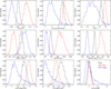 |
Fig. A.1. Marginalized parameters of the AC model. The panels contain the posterior probability density distributions, normalized to the maximum, for the phase-averaged (black lines), ON-pulse (red lines), and OFF-pulse (blue lines) spectra. The red lines mark the 5%, 50% (cross-section), and 95% percentiles of the 1D distributions. |
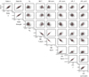 |
Fig. A.3. Marginalized parameters of the AC model. For the distributions of Fig. A.1 we have plotted the 2D histograms for each pair of parameters. |
Log-evidence for the MCAE and AC models as described in Sect. 4.
Best-fit values for the broadband χ2 fit of combined XMM-Newton and NuSTAR observation of NGC 300 ULX-1 for phase-average (FULL) spectra for the MCAE model without the Gaussian absorption line.
All Tables
Central values and confidence levels based on the marginalized parameter distribution of the Bayesian model comparison for the broadband fit of combined XMM-Newton and NuSTAR observation of NGC300 ULX-1 for phase-averaged (FULL) and phase-resolved spectra (ON- and OFF-pulse).
Best-fit values for the broadband χ2 fit of combined XMM-Newton and NuSTAR observation of NGC 300 ULX-1 for phase-average (FULL) spectra for the MCAE model without the Gaussian absorption line.
All Figures
|
Fig. 1. Data-to-model ratio vs. energy plot for the phase-averaged broadband (XMM-Newton plus NuSTAR) spectrum of NGC 300 ULX1. Top two panels: absorbed power-law models with exponential roll-off (using two different Xspec models). Two lower panels: AC and MCAE models, respectively. |
| In the text | |
|
Fig. 2. Structure of the accretion envelope. Optical depth at a distance. Across the envelope, the optical depth has been computed based on the minimum separation of the two confining lines. The separation of the lines (i.e., the base of the accretion column) has been selected to be 100 m (see discussion in West et al. 2017). |
| In the text | |
|
Fig. 3. Bottom panel: pulse profile of NGC 300 ULX1, using the 2016 XMM-Newton/EPIC-pn (black, and red lines; 0.3–10.0 keV) and NuSTAR data (green lines; 3.0–30.0 keV). ON-pulse and OFF-pulse spectra were extracted from the gray shaded areas, which have a width of 0.3 in phase. Top panels: XMM-Newton HR1: 0.3-2.0 vs. 2.0-4.5, HR2: 2.0–4.5 vs. 4.5–10.0, and NuSTAR HR3: 3.0–10.0 vs. 10.0–20.0. |
| In the text | |
|
Fig. 4. Unfolded spectra and data-to-model ratio plot of the ON-pulse, OFF-pulse, and FULL (phase-averaged) spectra from the MCAE modeling of the phase-averaged emission. |
| In the text | |
|
Fig. 5. Phase-averaged broadband (XMM-Newton plus NuSTAR) X-ray spectrum of NGC 300 ULX1 (upper panel) plotted together with the data-to-model ratio for the absorbed AC model (lower panel). For illustration purposes the strength of the absorption line has been set to zero. |
| In the text | |
|
Fig. 6. Marginalized parameters of the line depth (Kgabs, see Table 1 for details), temperature of the hot thermal component, and slope of power-law tail for the MCAE model. The red lines mark the 5%, 50% (cross-section) and 95% percentiles of the 1D distributions. For the distributions of Fig. A.1 we have plotted the 2D histograms for the two pairs of parameters (for the full parameter space, see Fig. A.4). |
| In the text | |
|
Fig. A.1. Marginalized parameters of the AC model. The panels contain the posterior probability density distributions, normalized to the maximum, for the phase-averaged (black lines), ON-pulse (red lines), and OFF-pulse (blue lines) spectra. The red lines mark the 5%, 50% (cross-section), and 95% percentiles of the 1D distributions. |
| In the text | |
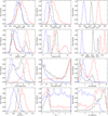 |
Fig. A.2. Same as Fig. A.1, but for the MCAE model. |
| In the text | |
|
Fig. A.3. Marginalized parameters of the AC model. For the distributions of Fig. A.1 we have plotted the 2D histograms for each pair of parameters. |
| In the text | |
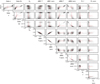 |
Fig. A.4. Same as Fig. A.3, but for the MCAE model. |
| In the text | |
Current usage metrics show cumulative count of Article Views (full-text article views including HTML views, PDF and ePub downloads, according to the available data) and Abstracts Views on Vision4Press platform.
Data correspond to usage on the plateform after 2015. The current usage metrics is available 48-96 hours after online publication and is updated daily on week days.
Initial download of the metrics may take a while.