| Issue |
A&A
Volume 649, May 2021
|
|
|---|---|---|
| Article Number | A116 | |
| Number of page(s) | 15 | |
| Section | Astrophysical processes | |
| DOI | https://doi.org/10.1051/0004-6361/201937335 | |
| Published online | 26 May 2021 | |
Using space-VLBI to probe gravity around Sgr A*
1
Institut für Theoretische Physik, Goethe Universität, Max-von-Laue-Str. 1, 60438 Frankfurt, Germany
e-mail: This email address is being protected from spambots. You need JavaScript enabled to view it.
2
Black Hole Initiative at Harvard University, 20 Garden Street, Cambridge, MA 02138, USA
3
Max-Planck-Institut für Radioastronomie, Auf dem Hügel 69, 53121 Bonn, Germany
4
Tsung-Dao Lee Institute and School of Physics and Astronomy, Shanghai Jiao Tong University, Shanghai 200240, PR China
5
Mullard Space Science Laboratory, University College London, Holmbury St. Mary, Dorking, Surrey RH5 6NT, UK
6
Department of Astrophysics/IMAPP, Radboud University Nijmegen, PO Box 9010 6500, GL, Nijmegen, The Netherlands
7
Anton Pannekoek Institute for Astronomy, University of Amsterdam, Science Park 904, 1098 XH, Amsterdam, The Netherlands
8
Dipartimento di Fisica “E. Pancini”, Universitá di Napoli “Federico II”, Via Cinthia, 80126 Napoli, Italy
9
INFN Sez. di Napoli, Via Cinthia, 80126 Napoli, Italy
10
Jodrell Bank Centre for Astrophysics, University of Manchester, Manchester M13 9PL, UK
11
Frankfurt Institute for Advanced Studies, Ruth-Moufang-Strasse 1, 60438 Frankfurt, Germany
12
School of Mathematics, Trinity College, Dublin 2, Ireland
Received:
17
December
2019
Accepted:
18
January
2021
Abstract
Context. The Event Horizon Telescope (EHT) will soon provide the first high-resolution images of the Galactic Centre supermassive black hole candidate Sagittarius A* (Sgr A*), enabling us to probe gravity in the strong-field regime. In addition to studying the accretion process in extreme environments, the obtained data and reconstructed images could be used to investigate the underlying spacetime structure. In its current configuration, EHT is able to distinguish between a rotating Kerr black hole and a horizon-less object such as a boson star. Future developments can increase the ability of EHT to tell different spacetimes apart.
Aims. We investigate the capability of an advanced EHT concept, including an orbiting space antenna, to image and distinguish different spacetimes around Sgr A*.
Methods. We used general-relativistic magneto-hydrodynamical simulations of accreting compact objects (Kerr and dilaton black holes as well as boson stars) and computed their radiative signatures via general-relativistic radiative transfer. To facilitate a comparison with upcoming and future EHT observations, we produced realistic synthetic data including the source variability, diffractive, and refractive scattering while incorporating the observing array, including a space antenna. From the generated synthetic observations, we dynamically reconstructed black hole shadow images using regularised maximum entropy methods. We employed a genetic algorithm to optimise the orbit of the space antenna with respect to improved imaging capabilities and u − v-plane coverage of the combined array (ground array and space antenna) and developed a new method to probe the source variability in Fourier space.
Results. The inclusion of an orbiting space antenna improves the capability of EHT to distinguish the spin of Kerr black holes and dilaton black holes based on reconstructed radio images and complex visibilities.
Key words: gravitation / magnetohydrodynamics (MHD) / radiation mechanisms: thermal / methods: numerical / techniques: interferometric / galaxies: individual: Sgr A*
© ESO 2021
1. Introduction
The Event Horizon Telescope (EHT) presented the first horizon scale images of the black hole in M 87 (Event Horizon Telescope Collaboration 2019a) and will soon provide the first image of the black hole candidate Sgr A* in our Galaxy. The current configuration of EHT consists of eight telescopes scattered across Europe, North and South America, and the South Pole (Event Horizon Telescope Collaboration 2019b). Combining the data recorded simultaneously by the individual telescopes after the observations, μas angular resolution is achieved. These observations enable us, for the first time, to study accretion processes in M 87 and in the centre of our Galaxy with unparalleled resolution and to probe gravity in the strong-field regime. Given the small number of telescopes participating in the observations, the intrinsic variability of the source, and the interstellar scattering screen, reconstructing an image and discriminating between different spacetimes is challenging (Lu et al. 2014, 2016; Mizuno et al. 2018). An interferometer such as the EHT samples the brightness distribution of an astronomical object in Fourier-space, the so called u − v plane. Due to the limited number of participating telescopes, the u − v plane is sparsely sampled. The sampling of this u − v plane increases with the number of telescopes and the duration of the observations. However, an improvement in the resolution of the image can only be obtained by increasing the distance between the telescopes, the so-called baselines, or by increasing the observed frequency. Given the current configuration of the EHT array, a significant increase in the baselines can only be achieved by extending baselines to space. Using the ground array while increasing the observed frequency above 345 GHz is limited by the opacity of the atmosphere and its water vapour content.
The concept of space-based Very Long Baseline Interferometry (VLBI) including a ground array has been studied extensively since the early 1970s (see Schilizzi 2012, for a historic overview). Successfully launched space antennas are the Highly Advanced Laboratory for Communications and Astronomy (HALCA; project VLBI Space Observatory Programme, VSOP; Hirabayashi et al. 1998) and, more recently, Spektr-R (project RadioAstron; Kardashev et al. 2013). Both missions operate at lower frequencies than EHT (230 GHz) and in the case of RadioaAstron provide μas resolution (Gómez et al. 2016). Therefore, in this work we consider the increase in the angular resolution that can be obtained by extending the baselines of EHT via a space-based antenna (see also Palumbo et al. 2019). This configuration has the advantage of using a well-calibrated ground array. For a mission based entirely on space telescopes, see the recent studies by Roelofs et al. (2019) and Fish et al. (2020). Within this work we address the scientific question as to whether such a configuration will improve the current ability of EHT to distinguish between different theories of gravity using radio observations of Sgr A*.
The structure of this paper is as follows: In Sect. 2 we briefly introduce our General Relativistic Magneto-Hydrodynamic (GRMHD) simulations and General Relativistic Radiative Transfer (GRRT) calculations. The procedure for the selection of the orbit of the space antenna is introduced in Sect. 3 and the results of the synthetic imaging and data analysis are shown in Sect. 4. We present our discussion and conclusions in Sect. 5 that Sgr A* is located at RA: 17h 45m 40.0409s and Dec: −29° 45′ 40.0409″, at a distance of 8178 ± 13 stat. ± 22 sys. pc, and its central candidate supermassive black hole (SMBH) exhibits a mass of Mbh = 4.14 × 10⁶ M⊙ (GRAVITY Collaboration 2019).
2. GRMHD and GRRT simulations
We used the state-of-the-art GRMHD code BHAC (Porth et al. 2017; Olivares et al. 2019) and performed three-dimensional accretion simulations on Kerr black holes (a* = 0.6 and a* = 0.94), dilaton black holes, and a boson star (Mizuno et al. 2018; Olivares et al. 2020). Here, a* is the dimensionless black-hole spin parameter, with |a*|< 1.
We have chosen a black hole solution in the Einstein–Maxwell–dilaton–axion (EMDA) theory, which derives from a particular string theory (Okai 1994; García et al. 1995). Such black-hole solutions exhibit more diverse physical properties than others in the literature. For example, they have hair, in addition to mass, rotation, and charge, thus they are an interesting laboratory for performing black hole experiments and studying possible differences between Einstein’s gravity and alternative theories of gravity. Moreover, since both the dilaton and the axion are considered to be candidates for dark matter, the study of the shadow from a dilaton black hole may provide hints as to the observational properties of the matter in which the black hole is immersed (Davoudiasl & Denton 2019).
We also consider a stable boson star, which although being classified as a compact object, is physically completely different from a black hole (Schunck & Liddle 1997). It is well known that the gravitational field of a boson star bends light around itself, creating a region resembling the shadow of a black hole’s event horizon. Similar to a black hole, a boson star accretes ordinary matter from its surroundings, but its opacity means that this matter, which would likely heat up and emit radiation, would be visible at its centre. There is no significant evidence so far that such stars exist. However, it may become possible to detect them through VLBI measurements (Olivares et al. 2020). In theory, a super-massive boson star could exist at the core of a galaxy, which might explain many of the observed properties of active galactic nuclei. Boson stars have also been proposed as candidate dark matter objects, and it has even been hypothesised that the dark matter haloes surrounding most galaxies might be viewed as enormous boson stars (Levkov et al. 2018).
The formation of boson stars or other exotic objects is an interesting process to study. Although we know that at the centre of our Galaxy there is a highly compact object, it is important to study different candidates because we might find that other galaxies could harbour exotic objects composed of ‘non-baryonic’ matter at their centres (Lee & Koh 1996).
For spacetimes not described by Einstein’s general theory of relativity, we used the Rezzolla–Zhidenko metric parameterisation (Rezzolla & Zhidenko 2014; Konoplya et al. 2016; Younsi et al. 2016). The initial conditions of all GRMHD simulations for Kerr and dilaton black holes as well as for the boson star consist of a torus in hydrodynamical equilibrium with a weak poloidal magnetic field. In order to trigger the accretion process, the magnetic field in the torus is seeded with a small perturbation which leads to the formation of the magneto-rotational instability (MRI). After the saturation of the MRI (t > 5000 GM/c2, with gravitational constant, G, mass of the central object, M, and speed of light c), all simulations show a quasi-stationary accretion flow (for more details see Mizuno et al. 2018; Olivares et al. 2020).
In the next step, we computed the radiative signature of the accretion process via GRRT calculations using the BHOSS code (Younsi et al. 2012, 2020; Gold et al. 2020). We used a viewing angle of θ = 60°, adjusted the ion-to-electron temperature ratio (Ti/Te = 3), and the mass-accretion rate in order to obtain the an average flux of 4 Jy at 230 GHz (see supplemental information in Mizuno et al. 2018, for a detailed description of the GRRT calculations and fitting procedure). This leads to a flux density variation between 3 Jy and 5 Jy (see light curve in the bottom panel of Fig. 1), which is in agreement with the observed flux density variations 2 Jy–5.5 Jy provided by Bower et al. (2015). The GRRT images were computed every 10 M, which corresponds to 200 s for Sgr A* for a time span of 4320 M (24 h for SgrA). This long duration allowed for the calculation of several overlapping and two independent 12 h1 observational windows. In this work we investigate the following spacetimes: Kerr black holes in general relativity, a dilaton black hole, and a boson star. The variability of the total flux and in the emission structure of the individual GRRT snapshots, together with the averaged image, is presented in Fig. 1. Additionally, in Table 1, we present an overview of the GRRT images used.
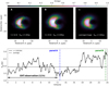 |
Fig. 1. Top, panels A and B: GRRT images for a Kerr black hole with a* = 0.6 including scattering effects (diffractive and refractive scattering) for two selected times t = 12.6 h and t = 23.6 h (dash-dotted line in the bottom panel) at a frequency of 230 GHz. The average image for 24 h of observation is presented in panel C. Bottom: simulated total flux light curve at 230 GHz for 24 h of observations. A typical EHT observation with a duration of 12 h is indicated. |
Overview of simulations used.
3. Orbit selection and optimisation strategy
In this section of our exploratory paper, we present one possible array optimisation strategy which could lead to improved imaging capabilities for EHT and thus may allow us to distinguish between different spacetimes. Thus, the question arises as to which kind of orbit is required for improving the imaging of the Galactic Centre. The answer to this question depends strongly on the observational constraints: the position of the Galactic Centre relative to the space and ground antennas and the duration of the observations. In the following, we assume an observation schedule consisting of 12 h of Sgr A* observations. This long observing time allows European as well as North and South American telescopes to participate in the observation.
For the space-EHT concept, we consider the EHT 2017 configuration as the ground array and include the Northern Extended Millimetre Array (NOEMA2) and a space antenna. In Table 2, we list each antenna and its corresponding system equivalent flux density (SEFD; Event Horizon Telescope Collaboration 2019b).
Effective antenna diameter d (for single telescopes this corresponds to the diameter of the dish) and system equivalent flux density (SEFD) used for the ground and space antennas (see Event Horizon Telescope Collaboration 2019b, for details).
For the orbiting space antenna, we assume a diameter of 8 m (similar to the size of Spektr-R), a system temperature of 100 K, and an antenna efficiency of 40%. Given these values, an SEFD of 20 × 103 Jy was computed. The orbit of the space antenna can be described by six orbital elements which can be divided into orbital shape parameters (semi-major axis, a, and eccentricity, e) and orbital orientation parameters, which provide the location and orientation of the orbit in space relative to the equatorial plane (inclination, i, longitude of the ascending node, Ω, argument of perigee, ω, and the true anomaly, ϑ). The six orbital elements of the space antenna together with the duration of the observations lead to a seven-dimensional parameter space, which has to be searched to obtain an optimal configuration. This task can be formulated as a constrained non-linear optimisation problem and written as follows:
 (1)
(1)
where x is a seven-dimensional vector containing the model parameters, that is, x ≡ [tobs,a,e,i,Ω,ω,ϑ]T, f(x) is the objective function (minimisation function), gj(x) are the constraints, and xL, i and xR, i are the lower and upper boundaries for the model parameters. In Table 3, we report the boundaries used during the optimisation.
Parameter boundaries used for the optimisation.
Improving the imaging capabilities of EHT can be translated into an increased angular resolution and a denser sampling of the u − v plane as compared to the current EHT configuration. The improvement of the imaging capabilities, that is to say better array resolution and u − v plane coverage, can be assessed by computing image metrics between the infinite resolution GRRT image and the reconstructed image. Therefore, for the minimisation process, we used a combination of the denser sampling in the u − v plane (minimising the distance between u − v points) and the improved imaging (improved image metrics). For the image metrics, we used the normalised cross correlation coefficient (nCCC) and the structural dissimilarity measure (DSSIM)3 (Wang et al. 2004). The minimisation function is given by:
 (2)
(2)
and we used the following constraints4 to speed up the optimisation procedure:
 (3)
(3)
 (4)
(4)
The first constraint ensures that the DSSIM is improved by at least 25% as compared to the image reconstructed using the EHT 2017 configuration. The denser sampling of the u − v plane is addressed by the second constraint, g2, where we enforced that the projected distance between the u − v points, Δr, was minimised with respect to the u − v sampling of the EHT 2017 configuration. During the optimisation, we generated for each set of parameters, (x), synthetic visibility where we included both diffractive and refractive scattering (Johnson 2016), and we reconstructed the image using the EHTim package5 (Chael et al. 2016, 2018).
Due to the numerical costs, during the optimisation, we used a single GRRT image instead of a series of GRRT images (or GRRT movie) and the array configuration and additional parameters used during the data generation and image reconstruction are listed in Tables 2 and 4. The procedure of the image reconstruction follows the approach of Chael et al. (2016): initialisation of the imaging using as Gaussian prior with a FWHM of 70 μas and the repeated re-initialisation of the imaging using the previously obtained image convolved with half the nominal array resolution. During the orbit optimisation, we used two re-initialisation loops and we aligned the reconstructed image with the GRRT image prior to the computation of the DSSIM.
Parameters used for the data generation and image reconstruction.
Given the high dimensionality of this constrained optimisation problem, gradient-based solvers may become stuck in a local minimum and/or may be required large computational resources to map out the gradient of the parameter space with sufficient resolution to avoid this problem. An elegant method to circumvent the above mentioned difficulties is based on gradient-free optimisation algorithms. For the purposes of this work, we applied a genetic algorithm (GA) and in particular employed the implementation of a Non Sorting Genetic Algorithm II (NSGA2) to solve the optimisation problem (Deb et al. 2002). For the initial generation, we used 1000 randomly initiated orbits and we evolved them for 100 generations.
The results of our numerical optimisation are presented in Table 5 and Fig. 2. The improvement of the image reconstruction is clearly visible by comparing the EHT 2017 reconstructed image (panel b in Fig. 2) with the image obtained by space-EHT (panel c in Fig. 2). The ground truth GRRT image is presented in panel a in Fig. 2. The space-EHT image is able to capture and image fine flux arcs which are smeared out in the EHT 2017 configuration. The visible image improvements are also reflected in the improved image metrics: The nCCC increased from 0.92 to 0.96 and the DSSIM decreased by 40% from 0.252 to 0.152 (see also constraint g1 Eq. (3)). It is important to notice that increased nCCC and decreased DSSIM correspond to better image matching. The satellite orbit as seen from Sgr A* (we note that the Earth is viewed from −30°) is presented in panel d in Fig. 2. In panel e in Fig. 2, the satellite ground track (projection of the satellite orbit onto the surface of the Earth) of the space antenna (red points for 12 h and grey ones for 24 h) and the ground antennas are indicated by the blue points. The sampling of the u − v plane is presented in panel f in Fig. 2 where the white points indicate the u − v tracks of the ground array and the red points indicate the u − v tracks including the space antenna. The addition of the space antenna does not only extend the u − v sampling up to 25 Gλ, but also adds short and intermediate baselines to the array as required by the constraint g2 (see Eq. (4)) of the optimisation process which also improve the imaging capabilities.
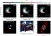 |
Fig. 2. Result of the orbit optimisation for 12 h of Sgr A* observations. Top row, from left to right: GRRT image (panel a), reconstructed image with interstellar scattering (including both diffractive and refractive scattering during the generation of the synthetic visibilities) using the EHT 2017 configuration convolved with 75% (red shading) of the nominal array resolution (light grey shading, panel b) and reconstructed image with interstellar scattering (including both diffractive and refractive scattering during the generation of the synthetic visibilities) using the space-EHT configuration convolved with 75% (red shading) of the nominal array resolution (light grey shading, panel c) for a dilaton black hole. Bottom row, from left to right: satellite orbit as seen from Sgr A* with orbital parameters and orbital period (panel d), satellite ground track (red lines for 12 h and grey ones for 24 h), ground array antennas (blue points, panel e), u − v sampling for the ground array (white points), and the baselines including the space antenna (red points, panel f). |
Optimised satellite orbit for 12 h of Sgr A* observation.
The orbit optimisation procedure suggested an elliptical orbit with a semi-major axis of a = 14 900 km with an eccentricity of e = 0.5 at an inclination of 67°. The optimal time span of the Sgr A* observation is obtained between 4:00 UT and 16:00 UT. The orbital period of the satellite is Tp = 5.03 h. It is important to notice that elliptical orbits with long orbital periods have also been used for VSOP (e = 0.6, Tp = 6.3 h) and the Spekt-R (e = 0.9, Tp = 200 h) (Hirabayashi et al. 1998; Kardashev et al. 2013). In Appendix A we illustrate the impact of different satellite orbits on the image reconstruction. Our results differ from the results of Palumbo et al. (2019), which used a circular orbit with semi-major axis a = 6652 km at an inclination of 61°. The similarity in the inclination is due to the declination (Dec) of Sgr A* of −29° and a face-on orbit is given by an inclination ∼Dec ± 90°. The difference in the eccentricity, e, and semi-major axis, a, can be explained by the different models used for Sgr A*. Palumbo et al. (2019) used a Schwarzschild black hole (a = 0) at an inclination of 10°. In this work, we used four different physical models: GR black holes (a = 0.6 and a = 0.94), a Dilaton black hole, and a boson star all at an inclination of 60°. Due to the larger relativistic effects at higher inclination (Doppler boosting), the GRRT images show a large left-right asymmetry for example, and the flux distribution is more compact as compared to black holes seen at an inclination of 10°. In addition, the boson star used in our work shows the most compact flux distribution around 10 μas (see panel i in Fig. 4). Since we require in our optimisation to resolve and recover the compact structure of the black holes and at the same time the boson star, we need to improve the angular resolution (longer baselines) and the u − v plane coverage (short baselines). Using one satellite, this can be achieved by an elliptical orbit. In our case the perigee is located at a height of ∼1100 km and the apogee at a height of ∼22 300 km. The space-ground tracks of this orbit are presented in panel f of Fig. 2 and the plot clearly shows the improved u − v coverage (short baselines with  and long baselines
  ).
).
Using this satellite orbit and the observing time span from 4:00 to 16:00 UT, the reconstructed images for all black holes and the boson star clearly improve the quality of the reconstructed images (better image metrics as compared to the EHT 2017 array) and are able to recover the structure seen in their infinite resolution GRRT counterparts (see Fig. 4).
After the optimisation of the space-EHT defining the orbit of the space antenna and the observing time, we created synthetic data taking the source variability during the course of the EHT observation into account. Therefore, for each of the spacetimes under investigation, we created a movie from the GRRT images which covers 12 h of observations (first 216 GRRT images are used, see indicated time 12 h time span in Fig. 1). From this movie, we created the synthetic visibilities using the same parameters used during the orbit optimisation (see Tables 2 and 4). As a consequence of creating the synthetic data from a variable source, the visibility amplitude (VA) of the zero baselines (ALMA-APEX, JCMT-SMA) is variable and not stationary as in the case when using a 12 h averaged GRRT image for the data creation. This behaviour is also true for non-zero baselines and for the closure phases (CP). In Fig. 3 we compare the VA and CP created from the GRRT movie and from its static average frame for the ALMA-SMT baseline and for the ALMA-LMT-SMT triangle. The differences in the behaviour of the VA and CP are clearly visible and the most striking difference can be seen at t = 10 UT.
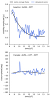 |
Fig. 3. Comparison between synthetic data generation from a dynamical movie (blue lines) and from its static average frame (black lines) for the visibility amplitude (top) and closure phase (bottom) for Kerr black hole with a* = 0.6. |
4. Results
Given the underlying variability in the flux density and also in the source size (see Fig. 1) of the different models, standard VLBI imaging approaches which assume a static source during the course of the observations are likely to fail at reconstructing an image. Therefore, we followed the approach of Johnson et al. (2017) and used dynamical imaging to reconstruct an average image from the time variable data. Since we are mainly interested in the average image obtained during the observation and our GRRT images do not show significant flaring events6, we used the ℛΔI regularizer with D2 distance metric and complex visibilities as a data product (see Johnson et al. 2017, for more details). We reconstructed 24 frames with a duration of 30 min each for a total duration of 12 h. For the first initialisation of the imaging, we applied a circular Gaussian with an FWHM = 70 μas prior image and for repeated re-initialisation of the imaging we used the previously obtained average image computed from all 24 frames convolved with half of the nominal array resolution as a prior. For the dynamical reconstruction, we applied five re-initialisation loops.
4.1. Image plane comparison
In order to quantify the ability to test different spacetimes, we computed the structural dissimilarity measure (DSSIM; Wang et al. 2004) between the GRRT and reconstructed images. Before computing the DSSIM, we performed an image alignment using the normalised cross correlation coefficient (nCCC; see Mizuno et al. 2018). Both image metrics are reported in the panels of Fig. 4 and in Table 6.
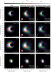 |
Fig. 4. Synthetic black hole images for Sgr A* for a Kerr black hole with a* = 0.94 (panels a–c), a Kerr black hole with a* = 0.6 (panels d–f), a non-rotating dilaton black hole (panels g–i), and for a stable, non-rotating boson star (panels j–l). From left to right and for all rows: GRRT image (panels a, d, g, j), dynamically reconstructed image with interstellar scattering (including both diffractive and refractive scattering during the generation of the synthetic visibilities) using the EHT 2017 configuration convolved with 75% (red shading) of the nominal beam size (light grey shading, panels b, e, h, k), and dynamically reconstructed image with interstellar scattering (including both diffractive and refractive scattering during the generation of the synthetic visibilities) using the space-EHT configuration convolved with 75% (red shading) of the nominal beam size (light grey shading, panels c, f, i, l). |
Results of the cross-comparison of the synthetic images using the EHT 2017 and the advanced EHT configuration.
In Table 6 we list the DSSIM and nCCC values computed for the different image combinations and for the different array configurations. If we could clearly distinguish between different theories based on the reconstructed images, the smallest DSSIM and largest nCCC values should be obtained for equal image pairs, or for example for boson stars (the diagonal in Table 6). However, for the EHT 2017 configuration, this is only true for the boson star. Thus based on reconstructed images obtained from synthetic data which take the source variability into account, it is difficult for the EHT 2017 configuration to distinguish the spin of Kerr black holes and to differentiate a Kerr black from a dilaton black hole (see very similar values in Table 6). Including a space antenna improves the ability to distinguish between the different spacetimes, especially for the Kerr black hole with high spin. Given the obtained image metrics, the space-EHT concept can distinguish the spin of the Kerr black holes, but it is still difficult to discriminate between a Kerr black hole with spin a* = 0.6 and a dilaton black hole (see Table 6).
By comparing the image metrics obtained for EHT 2017 and the space-EHT concept, the following two different behaviours can be found: improved image metrics (decreased DSSIM and increased nCCC) and worsened ones (increased DSSIM and decreased nCCC). For equal image pairs dilaton–dilaton, the image metrics for the space-EHT concept improved as compared to the EHT 2017 (as discussed above). However, for unequal image pairs, there are two different behaviours. For example in the boson star and dilaton case, the image metrics improved. In contrast to the dilaton–boson star pair where the image metrics become worse. This behaviour could be understood in the following way: The boson star image is very compact as compared to the dilaton model (see left column in Fig. 4). Due to the limited resolution of the EHT 2017 array, the intrinsically large structure of the dilaton model is smeared and scattered out to an even larger structure (compare panel i and j in Fig. 4). However, the improved imaging capabilities of the space-EHT concept leads to a more compact and less smeared out source structure, which is reflected by a better matching between the boson star and the dilaton black hole. The contrary happens in the dilaton–boson star case: The EHT 2017 blurs the true boson star structure to a large size which matches the dilaton structure better as compared to a sharper, more compact boson star image provided by the space-EHT concept. As a result, the image metrics for this image pair will worsen as compared to the EHT 2017. A similar behaviour can be seen for Kerr a* = 0.6–boson star and to some extent for dilaton–Kerr a* = 0.94 and Kerr a* = 0.6–Kerr a* = 0.94. In Appendix B we provide a more detailed study on the variation of the image metrics with respect to intrinsic source size and array resolution.
4.2. Fourier plane comparison
Given that an interferometer measures the Fourier transform of the brightness distribution of an astronomical source, a more direct comparison between images of different spacetimes can be obtained in Fourier space. The turbulent nature of the accretion process in the GRMHD simulations manifests itself in large variations in the total flux density and in its flux density distribution (see Fig. 1 for Kerr a* = 0.6). In this work we include the variability of the source in the scoring procedure. Therefore we modified the scheme used in Event Horizon Telescope Collaboration (2019c) for the analysis of the recent EHT M 87 observations. The main modification is that for the comparison with the synthetic data, we used a GRRT movie generated from a series of GRRT images spanning the observing time given by the synthetic data set. For the purposes of this work, typically 216 frames (for an EHT observation of 12 h) were used and we slid along our GRRT data series for the different spacetimes where an increment of five frames was used. The increment of five frames is justified by the fact that the typical correlation times of the GRRT images are around 50 M. This implies that around this time, the GRRT images can be regarded as independent realisations of the accretion flow and thus the different movies created from the sliding window can be considered as uncorrelated. The first step in the scoring procedure is to create complex visibilities from the GRRT movie, taking into account the array configuration, the observing schedule, and interstellar scattering, including both diffractive and refractive scattering (see also Tables 2 and 4). From the complex visibilities, we computed the visibility amplitude (VA) and from closed antenna triangles we computed the closure phase (CP). The latter is of great importance in measuring the structural variation within the source. In the second step, we minimised the χ2 for VA and CP between the snapshots and the individual frames (images) of the GRRT movie by allowing the total flux, the position angle, and the black hole mass7 to vary. It is important to notice that once the values for the flux scaling, position angle, and black hole mass were set, they were kept constant for all frames of the GRRT movie in order to ensure the consistency of the movie. In addition to the image scaling, we performed antenna gain calibrations. We limited the variation in the individual antenna gains to between 50% and 150% in order to avoid the compensation of structural differences among the models by large gain variations. The scoring was carried out with the well tested GENA pipeline developed for the image matching of EHT and VLBA observations (Event Horizon Telescope Collaboration 2019c,d; Fromm et al. 2019), and we focussed our analysis on the synthetic observations including a space antenna. The scheme for this kind of scoring which includes the source variability (hereafter movie scoring) is illustrated in Fig. 5.
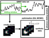 |
Fig. 5. Illustration of the movie scoring scheme. From the GRRT data, via a sliding window, we selected a set of images from which a movie was created. From this movie, complex visibilities were generated and the χ2 between the synthetic data was computed while allowing the movie to rotate and vary in source size and flux density. The χ2 were minimised either using an evolutionary algorithm (EA) or an MCMC scheme. After the optimisation, the sliding window was advanced until the entire GRRT data set was sampled. |
In Fig. 6 we show an example of movie scoring for Kerr a* = 0.94 synthetic data to the Kerr a* = 0.94 model. The obtained values for the mass, flux scaling, and position angle are indicated in the top panel. The recovered values are in good agreement with the injected values. A more detailed self-test of the movie scoring scheme is presented in Appendix C.
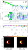 |
Fig. 6. Scoring result of the Kerr a* = 0.94 synthetic data to the Kerr a* = 0.94 model. The panels show from top to bottom the visibility amplitude, the closure phase, the calibrated gains, and the average image of the Kerr a* = 0.94 movie (GRRT left and convolved right). |
During our analysis, we fitted the synthetic data generated from the first 12 h of our GRRT data set to the entire data by advancing the sliding window with an increment of five frames. This allowed us to statistically quantify the difference between the synthetic data generated from the first 12 h to the entire GRRT data set including the source variability. In the next step, we kept the synthetic data and scored it against the GRRT images of the three different remaining spacetimes. Finally, we obtained the χ2-distribution for VA, CP, the position angle (measured from north to east), and the mass distribution for various combinations of synthetic data and the entire GRRT image sets for different spacetimes. Based on these distributions, we performed a Kolmogorov–Smirnov (K–S) test to determine if the synthetic data under investigation are in agreement with being drawn from one of the four spacetimes.
Here, we provide a short example which explains the generation of the violin plots and the obtained p-value from the K–S test. In assuming two normal distributions, one with a mean at 5.5 and a standard deviation of 0.25 and another one with a mean at 5.7 and a standard deviation of 0.35, then, one can draw 20 random numbers for the distribution and create a violin plot (the left half of the violin is the histogram for the first distributions and the right half corresponds to the second distribution). In this case, the violin looks nearly symmetrical with only a slight shift and the computed K–S test provides a p-value of 0.49. This value implies that the hypothesis that the values are from the same ‘overall’ distribution cannot be rejected or that the underlying model (spacetime) is the same (see left most violin in the top panel of Fig. 7). On the contrary, if the mean of the second distribution is located at 12, the two wings of the violin are disjoint and the K–S test provides a p-value of 5 × 10⁻¹⁰. This value indicates that the two distributions are not draw from the same ‘overall’ distributions. This would imply that the underlying model (spacetime) is not the same (see right most violin in Fig. 7).
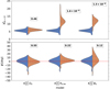 |
Fig. 7. Results for the Kerr a* = 0.6 test. The panels show the distribution of the total |


In the following, we label the different spacetimes by their first letter and a subscript indicates their spin, for example K0.6 for a Kerr black hole with spin a* = 0.6. We indicate the synthetic data by a superscript ‘syn’, for example  for the synthetic data of the Kerr black hole with spin a* = 0.6 generated from the first 12 h. Using this notation, scoring the synthetic data Kerr a* = 0.6 against the entire data set of Kerr a* = 0.94 is given by
  .
.
4.2.1. Application to Kerr a* = 0.6 (test 1)
In the first application of the movie scoring technique, we wanted to test whether we could distinguish the synthetic data for a Kerr black hole with spin a* = 0.6 from a Kerr black hole with spin a* = 0.94, a dilaton black hole, and from a boson star. Therefore, we scored the synthetic data for Kerr black with spin a* = 0.6 against the data set for the different spacetimes and performed the KS test. Given the known black hole mass for the black hole in Sgr A⋆ and its small uncertainty from the GRAVITY experiment (GRAVITY Collaboration 2019), we kept the black hole mass fixed for this first test and performed the K-S test only on the total  and the position angle.
Figure 7 shows the results for the Kerr a* = 0.6 test. For K0.6 − D0, the χ2 shows a very similar, only slightly shifted shape. In contrast to K0.6 − K0.94 and K0.6 − B0 where the distributions are only marginally overlapping. The distributions for the position angle ϕ overlap with the distribution of the truth model ( , blue violins) in all cases. This behaviour can be explained by the very similar source size for the Kerr a* = 0.6 and dilaton black hole in contrast to the Kerr black hole with spin a* = 0.94 and the boson star (see left column in Fig. 4). In order to improve the χ2 during the optimisation (or MCMC) step, the image was rotated a bit more in the case of the Kerr a* = 0.94 and the boson star data set. The results of the K–S test can be found in Table 7. The results of the movie scoring indicate that the space-EHT concept can clearly distinguish fast from slow spinning black holes as well as from boson stars.
Results of the K–S tests for Kerr a* = 0.6 and Kerr a* = 0.9 as truth images.
4.2.2. Application to Kerr a* = 0.94 (test 2)
For the second test, we used the synthetic data from the Kerr black hole with spin a* = 0.94 and we tested if it can be distinguished from either a Kerr black hole with spin a* = 0.6, a dilaton black hole, or a boson star. The following movie scorings were computed:  (synthetic data and GRRT data set are from the same spacetime),
  ,
,  , and
, and  . The χ2 and position angle distribution of all test pairs of models are clearly shifted (see Fig. 8). This behaviour is also reflected in the small numbers for the K–S test (see Table 7). The shift in the χ2 distributions can be explained by the difference in source size for the Kerr a* = 0.6 and dilaton black hole. In order to match the source size of the Kerr black hole with spin a* = 0.94, the dilaton and Kerr black hole with spin a* = 0.6 would require a smaller black hole mass mbh < 4.14 × 10⁶ M⊙. Since we did not allow the black hole mass to adjust, the only way to improve the χ2 would be to rotate the GRRT movies. An improved χ2 was obtained by rotating the GRRT movies and the mean of the ϕ distributions is located at −15° (Kerr black hole with spin a* = 0.6) and −25° (dilaton black hole). Similarly, the boson star would require a larger black hole mass to fit the Kerr a* = 0.94 synthetic data. Given the distributions and the result of the K–S test, the space-EHT concept can distinguish between all three models if the truth model is a Kerr black hole with spin a* = 0.94.
4.2.3. Application to Kerr a* = 0.6 with varying black hole mass (test 3)
In order to test the variations in the black hole mass required to make the Kerr a* = 0.6 indistinguishable for the space-EHT concept from the dilaton black hole, we performed a third test where we restricted ourselves to Kerr a* = 0.6 and dilaton black holes and allowed the black hole mass to adjust during the optimisation. The result for this test is presented in Fig. 9. As expected, the adjusted black hole mass for the dilaton black hole improved the p-values for the K–S test on all quantities ( , ϕ, and mbh). However, this would require a black hole mass of mbh = 4.05 × 10⁶ M⊙, which is not in agreement with the current measurements of GRAVITY (GRAVITY Collaboration 2019).
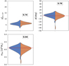 |
Fig. 9. Results for the Kerr a* = 0.6–dilaton black hole test with varying black hole mass. The panels show the distribution of the total |


5. Discussion and summary
In this exploratory paper, we address the question if an orbiting space antenna will improve the capabilities of the EHT to distinguish between different spacetimes around Sgr A*. Our proposed optimisation procedure has suggested an elliptical orbit with an eccentricity of e = 0.5 and a semi-major axis of a = 14 900 km. By including the suggested space antenna, the baselines of the EHT array could be extended beyond 10 000 km and thus increase the angular resolution and the imaging capabilities of the array considerably (see right column in Fig. 4). As can be seen in Table 6, the space-EHT is able to distinguish the spin of Kerr black holes (best image metrics can be found for equal image pairs). For example, the DSSIM for the Kerr a* = 0.6–Kerr a* = 0.6 dropped from 0.13 to 0.10, while the Kerr a* = 0.6–Kerr a* = 0.94 is 0.12. The improvement on the imaging capabilities of the space-EHT is also noticeable in the change of the computed nCCC: For Kerr a* = 0.6, the nCCC increased from 0.92 to 0.96; while for the Kerr a* = 0.94 case, the nCCC decreased from 0.94 to 0.91. A similar behaviour is found for the other equal image pairs Kerr a* = 0.94–Kerr a* = 0.94 as compared to the non-equal image pairs Kerr a* = 0.94–boson star (see last row in Table 6). For the a* = 0.6 Kerr black hole and the dilaton black hole comparison, the DSSIM value decreased from 0.13 to 0.10 and the nCCC increased from 0.92 to 0.96. Given the very similar numbers for Kerr a* = 0.6–Kerr a* = 0.6 and dilaton–dilaton it is currently not possible to distinguish between both spacetimes based solely on their reconstructed images.
To circumvent the limitations of reconstructed average images in distinguishing between different theories of gravity, we additionally performed a detailed comparison in Fourier space including the source variability. We created synthetic data from the first 12 h of the GRRT images of the two different Kerr black holes and scored them against 12 h movies created from the GRRT images of all four spacetimes. Fitting the synthetic data for the Kerr black hole with spin a* = 0.6 against its entire GRRT data set leads to a χ2 distribution with a mean value of 5.6 and a standard deviation of 0.5 (see blue violins in Fig. 7). The position angle distribution peaks at a value of ϕ = 0.7° ±4°. This value is close to the initial value we used for the creation of the synthetic data and can be regarded as a confirmation of the fitting routine.
We performed two-sided K–S tests to investigate the hypothesis that the synthetic data are drawn from a spacetime other than Kerr. The result for the Kerr a* = 0.6 tests reveal very small numbers for the synthetic data generated from Kerr a* = 0.9 and a boson star, both for the χ2 and for the position angle (see Fig. 7 and Table 7). Thus we could reject the null-hypothesis and conclude that Kerr a* = 0.9 and a boson star can be distinguished from an a* = 0.6 Kerr black hole. The K–S test between the a* = 0.6 Kerr and the dilaton black holes provides values that are significantly larger than for the Kerr a* = 0.94 and a boson star. The mean values of the dilaton distributions are shifted by roughly one standard deviation compared to the truth distribution (Kerr a* = 0.6). Given the obtained values, it is likely (54% level) that we can distinguish an a* = 0.6 Kerr black hole from a dilaton black hole. In an additional test, we allowed the black hole mass to adjust and in order to probe the mass variation which would lead to undistinguishable data sets, for example, we could not differentiate between a Kerr black hole with spin a* = 0.6 and a dilaton black hole. The shift between the χ2 and ϕ distribution decreased which leads to larger p-values for the K–S test (see Table 7 and Fig. 9). In addition to the previous test, we also obtain the distribution for the black hole mass. The obtained mean black hole mass for the Kerr black hole with spin a* = 0.6 is  , which is in good agreement with the black hole mass used during the radiative transport calculations and a confirmation of the movie scoring method. In order to make both theories of gravity undistinguishable to 74%, the mean black hole mass should decrease to mbh = 4.02 × 10⁶ M⊙. However, given the mass boundaries from the GRAVITY experiment, this black hole mass is outside the allowed range. Similar to the a* = 0.6 Kerr case, we performed K–S tests on the fast spinning Kerr black hole with a* = 0.94. Again, we obtain the distribution for the χ2 and the position angle ϕ and computed the K–S test. All distributions for this test are clearly offset from the truth distribution (see top panel in Fig. 8), which is also reflected in the very small numbers obtained for the p-value (see Table 7). However, given the small p-values, we conclude that the fast-spinning Kerr black hole can be clearly distinguished from the slower spinning Kerr black hole, the dilaton, and the boson star.
In summary, we have presented a future EHT concept which includes a space antenna and tested the capabilities of this new array to investigate the different possible spacetimes around Sgr A* via radio images and complex visibilities. The orbit of the satellite was computed from a non-linear optimisation using a genetic algorithm and constraints on the u − v-plane filling, observation time, and improved image metrics computed between the GRRT image and the reconstructed image. We generated synthetic data for three different theories of gravity, namely the following: a Kerr black hole (general relativity), a dilaton black hole, and a boson star. The synthetic data generated were created from 12 h of a GRRT movie in order to properly include the source variability, and a dynamical image reconstruction was applied following Johnson et al. (2017) using ehtim. From the dynamical reconstructed images, an average image was computed and compared to the average frame of the GRRT movies using DSSIM and nCCC metrics. The image plane comparison was accompanied by a more detailed and robust analysis in the Fourier plane using the newly developed movie scoring method in GENA. A K–S test was performed on the χ2 position angle and mass distributions in order to investigate the possibility of distinguishing between different spacetimes and therefore different theories of gravity. The space-EHT concept presented in this study has been shown to both improve the imaging capabilities, while including the source variability of the array, and improve our ability to distinguish between (and potentially exclude) certain solutions a nd theories of gravity.
Our ability to image time-variable sources and probe the underlying spacetime will be further improved by the addition of more ground antennas, for example the African Millimetre Telescope (ATM; Backes et al. 2016) or several telescopes placed at dedicated locations across the globe as planed by the next generation EHT (ngEHT; Doeleman et al. 2019). Extending the GRRT images series will allow us to address the source variability on larger non-overlapping time windows, improving the statistics. Increasing the observing frequency (ν > 500 GHz) will reduce the interstellar scattering and also allow us to study general relativistic effects on horizon scales more deeply since the obtained image is less affected by the properties of the accretion flow and the radiation microphysics. However, due to the opacity of Earth’s atmosphere, such a concept would require an entirely space-based VLBI concept (see Roelofs et al. 2019; van der Gucht et al. 2020).
In addition to horizon scale images of the EHT and future space-EHT concepts, further constraints on the properties of the spacetime around Sgr A* can be obtained from a pulsar in a tight orbit (orbital period ∼1 yr ) around the galactic centre (Liu et al. 2012). When combined, both measurements, for example of horizon scale images and pulsar timing, would allow tight constraints on the properties of spacetime around Sgr A* (Psaltis et al. 2016).
Typical duration for EHT observations of Sgr A* which allows European and American telescopes to participate in the observation.
Smaller values indicate a better image agreement.
The constraints are fulfilled if the gi < 0.
We define a flare as the doubling of the flux density from one frame to another.
In fact, we varied the plate scale, μ = mbh/dbh, during the scoring. Assuming a fixed distance dbh to Sgr A*, we computed the black hole mass, mbh, from μ.
We applied a circular Gaussian.
Acknowledgments
CMF thanks E. Ros, R. Porcas and D. Palumbo for fruitful discussion and comments on the manuscript. Support comes from the ERC Synergy Grant “BlackHoleCam – Imaging the Event Horizon of Black Holes” (Grant 610058). CMF is supported by the black hole Initiative at Harvard University, which is supported by a grant from the John Templeton Foundation. ZY acknowledges support from a Leverhulme Trust Early Career Fellowship.
References
- Backes, M., Müller, C., Conway, J. E., et al. 2016, in The 4th Annual Conference on High Energy Astrophysics in Southern Africa (HEASA 2016), 29 [Google Scholar]
- Bower, G. C., Markoff, S., Dexter, J., et al. 2015, ApJ, 802, 69 [NASA ADS] [CrossRef] [Google Scholar]
- Chael, A. A., Johnson, M. D., Narayan, R., et al. 2016, ApJ, 829, 11 [NASA ADS] [CrossRef] [Google Scholar]
- Chael, A. A., Johnson, M. D., Bouman, K. L., et al. 2018, ApJ, 857, 23 [Google Scholar]
- Davoudiasl, H., & Denton, P. B. 2019, Phys. Rev. Lett., 123, 021102 [Google Scholar]
- Deb, K., Pratap, A., Agarwal, S., & Meyarivan, T. 2002, Trans. Evol. Comp., 6, 182 [Google Scholar]
- Doeleman, S., Blackburn, L., Dexter, J., et al. 2019, BAAS, 51, 256 [Google Scholar]
- Event Horizon Telescope Collaboration (Akiyama, K., et al.) 2019a, ApJ, 875, L1 [NASA ADS] [CrossRef] [Google Scholar]
- Event Horizon Telescope Collaboration (Akiyama, K., et al.) 2019b, ApJ, 875, L2 [NASA ADS] [CrossRef] [Google Scholar]
- Event Horizon Telescope Collaboration (Akiyama, K., et al.) 2019c, ApJ, 875, L6 [Google Scholar]
- Event Horizon Telescope Collaboration (Akiyama, K., et al.) 2019d, ApJ, 875, L5 [Google Scholar]
- Fish, V. L., Shea, M., & Akiyama, K. 2020, AdSpR, 65, 821 [Google Scholar]
- Foreman-Mackey, D. 2016, J. Open Source Softw., 1, 24 [Google Scholar]
- Foreman-Mackey, D., Hogg, D. W., Lang, D., & Goodman, J. 2013, PASP, 125, 306 [Google Scholar]
- Fromm, C. M., Younsi, Z., Baczko, A., et al. 2019, A&A, 629, A4 [NASA ADS] [CrossRef] [EDP Sciences] [Google Scholar]
- García, A., Galtsov, D., & Kechkin, O. 1995, Phys. Rev. Lett., 74, 1276 [NASA ADS] [CrossRef] [Google Scholar]
- Gold, R., Broderick, A. E., Younsi, Z., et al. 2020, ApJ, 897, 148 [Google Scholar]
- Gómez, J. L., Lobanov, A. P., Bruni, G., et al. 2016, ApJ, 817, 96 [Google Scholar]
- GRAVITY Collaboration (Abuter, R., et al.) 2019, A&A, 625, L10 [NASA ADS] [CrossRef] [EDP Sciences] [Google Scholar]
- Hirabayashi, H., Hirosawa, H., Kobayashi, H., et al. 1998, Science, 281, 1825 [NASA ADS] [CrossRef] [PubMed] [Google Scholar]
- Johnson, M. D. 2016, ApJ, 833, 74 [NASA ADS] [CrossRef] [Google Scholar]
- Johnson, M. D., Bouman, K. L., Blackburn, L., et al. 2017, ApJ, 850, 172 [NASA ADS] [CrossRef] [Google Scholar]
- Kardashev, N. S., Khartov, V. V., Abramov, V. V., et al. 2013, Astron. Rep., 57, 153 [Google Scholar]
- Konoplya, R., Rezzolla, L., & Zhidenko, A. 2016, Phys. Rev. D, 93, 064015 [NASA ADS] [CrossRef] [Google Scholar]
- Lee, J.-W., & Koh, I.-G. 1996, Phys. Rev. D, 53, 2236 [NASA ADS] [CrossRef] [Google Scholar]
- Levkov, D. G., Panin, A. G., & Tkachev, I. I. 2018, Phys. Rev. Lett., 121, 151301 [Google Scholar]
- Liu, K., Wex, N., Kramer, M., Cordes, J. M., & Lazio, T. J. W. 2012, ApJ, 747, 1 [CrossRef] [Google Scholar]
- Lu, R.-S., Broderick, A. E., Baron, F., et al. 2014, ApJ, 788, 120 [NASA ADS] [CrossRef] [Google Scholar]
- Lu, R.-S., Roelofs, F., Fish, V. L., et al. 2016, ApJ, 817, 173 [NASA ADS] [CrossRef] [Google Scholar]
- Mizuno, Y., Younsi, Z., Fromm, C. M., et al. 2018, Nat. Astron., 2, 585 [Google Scholar]
- Okai, T. 1994, Progr. Theoret. Phys., 92, 47 [Google Scholar]
- Olivares, H., Porth, O., Davelaar, J., et al. 2019, A&A, 629, A61 [NASA ADS] [CrossRef] [EDP Sciences] [Google Scholar]
- Olivares, H., Younsi, Z., Fromm, C. M., et al. 2020, MNRAS, 497, 521 [CrossRef] [Google Scholar]
- Palumbo, D. C. M., Doeleman, S. S., Johnson, M. D., Bouman, K. L., & Chael, A. A. 2019, ApJ, 881, 62 [Google Scholar]
- Porth, O., Olivares, H., Mizuno, Y., et al. 2017, Comput. Astrophys. Cosmol., 4, 1 [Google Scholar]
- Psaltis, D., Wex, N., & Kramer, M. 2016, ApJ, 818, 121 [Google Scholar]
- Rezzolla, L., & Zhidenko, A. 2014, Phys. Rev. D, 90, 084009 [NASA ADS] [CrossRef] [MathSciNet] [Google Scholar]
- Roelofs, F., Falcke, H., Brinkerink, C., et al. 2019, A&A, 625, A124 [NASA ADS] [CrossRef] [EDP Sciences] [Google Scholar]
- Schilizzi, R. 2012, Resolving The Sky - Radio Interferometry: Past, Present and Future, 10 [Google Scholar]
- Schunck, F. E., & Liddle, A. R. 1997, Phys. Lett. B, 404, 25 [Google Scholar]
- van der Gucht, J., Davelaar, J., Hendriks, L., et al. 2020, A&A, 636, A94 [EDP Sciences] [Google Scholar]
- Wang, Z., Bovik, A. C., Sheikh, H. R., & Simoncelli, E. P. 2004, IEEE Trans. Image Proces., 13, 600 [Google Scholar]
- Younsi, Z., Wu, K., & Fuerst, S. V. 2012, A&A, 545, A13 [NASA ADS] [CrossRef] [EDP Sciences] [Google Scholar]
- Younsi, Z., Zhidenko, A., Rezzolla, L., Konoplya, R., & Mizuno, Y. 2016, Phys. Rev. D, 94, 084025 [NASA ADS] [CrossRef] [Google Scholar]
- Younsi, Z., Porth, O., Mizuno, Y., Fromm, C. M., & Olivares, H. 2020, in Perseus in Sicily: From Black Hole to Cluster Outskirts, eds. K. Asada, E. de Gouveia Dal Pino, M. Giroletti, H. Nagai, & R. Nemmen, 342, 9 [Google Scholar]
Appendix A: Influence of the orbital parameters on the imaging capabilities
In Fig. A.1 we illustrate the impact of the orbital parameters on the imaging capabilities of the space-EHT concept and the trade-offs between u − v coverage and array resolution. We kept the orientation parameters of the orbit fixed to the results of our orbit optimisation (see Table 5) and changed the semi-major axis, a, and eccentricity, e.
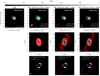 |
Fig. A.1. Reconstruction of a boson star image for Sgr A* (ground truth image in panel a) for the following three different satellite orbits: small orbit (second column), intermediate orbit (third column), and large orbit (fourth column). From top to bottom: reconstructed image convolved with 75% of the nominal array resolution, the uv-coverage (white: ground array baselines, red: space baselines), and the satellite orbit as seen from Sgr A*. |
An increase in the semi-major axis, a (see panel j in Fig. A.1), leads to higher resolution (see beam in panel d in Fig. A.1). At the same time, the larger semi-major axis, a, which corresponds to a larger orbital period  , reduces the u − v coverage (see panel g in in Fig. A.1). This leads to a worse image metric than a medium-sized orbit, for example (compare image metrics in panel c and d in Fig. A.1). On the other hand, a small semi-major axis (see panel h in Fig. A.1) leads to a dense u − v coverage (panel e in Fig. A.1), but it does not provide high angular resolution (see panel b in Fig. A.1). A trade-off between resolution and u − v coverage is an intermediate-sized semi-major axis (see third column in in Fig. A.1). For each of the three satellite orbits, the image metrics were calculated prioritising the orbit with the best image metrics, the orbit with a semi-major axis of a = 14 861 km, and an eccentricity of e = 0.5.
Appendix B: DSSIM and nCCC
In order to explore the variation of the DSSIM and the nCCC, we performed a small parameter space study using averaged GRRT images. The GRRT images are taken from Kerr BHs with spin a* = 0.6 and a* = 0.94 as well as from the dilaton black hole. To mimic different observing arrays with improved imaging capabilities, we convolved the average images with different beam sizes8 ranging from 30 μas to 1 μas. The convolved images were compared to the ground truth GRRT images and the DSSIM and the nCCC values were computed. In Fig. B.1 we show the results for this study. As expected, the DSSIM values decrease with smaller beam sizes, while the nCCC increases for all image pairs. However, at a beam size of ∼16 μas, the DSSIM values for the Kerr BH with a* = 0.94 increases and at the same time the nCCC decreases. This behaviour can be understood by the different source sizes of the ground truth images (see left most column in the top panel in Fig. B.1). The compact source structure of the Kerr BH with a* = 0.94 was smeared out to larger extents during the convolution with a beam with a size > 16 μas, which matches the ground truth structure better of the Kerr BH with a* = 0.6. Thus, the DSSIM decreases while the nCCC increases. However at a beam size of ∼16 μas, the behaviour is inverted. For the models with similar ground truth sizes, the DSSIM monotonically decreases while the nCCC continuously increases. If the size of the ground truth image is smaller than the intrinsic size of the models to which it is compared, for example for Kerr BH with a* = 0.94 and Kerr BH a* = 0.6, no change in the DSSIM and nCCC behaviour is found: the DSSIM is always decreasing and the nCCC is continuously increasing with decreasing beam size (see bottom panel in Fig. B.1).
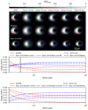 |
Fig. B.1. DSSIM and nCCC variation study. Top panel: ground truth images for Kerr a* = 0.6, Kerr a* = 0.94 and dilaton black holes (left most column) and convolved with decreasing beams (30 μas–1 μas). Middle panel: DSSIM and nCCC calculations using the average image of Kerr BH with a* = 0.6 as ground truth image. Bottom panel: DSSIM and nCCC calculations using the average image of Kerr BH with a* = 0.94 as ground truth image. |
Appendix C: Movie scoring self-test
To valid the developed movie scoring method, we performed a self-test. For the self-test, we generated synthetic visibilities from the Kerr black hole with spin a* = 0.94. The start frame for the synthetic data generation was shifted by 1.7 h (30 frames). During the generation of the synthetic data, we took interstellar scattering (including both diffractive and refractive scattering), thermal noise, and gain variations into account (see also Table 4). For a successful self-test, the movie scoring method should recover the correct starting frame, the black hole mass, and the orientation of the images used during the synthetic data generation. During the radiative transfer, we used a black hole mass of 4.14 × 10⁶ M⊙ and an orientation angle of ϕ = 0°. During the self-test, we allowed the black hole mass, mbh, the rotation angle, ϕ, and the flux normalisation, S, to adjust during the scoring. For the optimisation, we applied an MCMC method (Foreman-Mackey et al. 2013; Foreman-Mackey 2016) using 100 MCMC walkers for 500 iterations and performed gain-calibration.
The movie scoring method successfully recovered the start frame and in Fig. C.1 we present the posterior distribution for the black hole mass, the orientation angle, and the flux scaling for the GRRT movie starting at frame 30. The black hole mass and the orientation angle are recovered within 1σ proofing the applicability of the developed method to recover black hole parameters from a source with a varying flux density and structure. The posterior distribution of the flux scaling, Sscale, reflects the influence of interstellar scattering and antenna gain variations taken into account during the synthetic data generation. Interstellar scattering smears out the flux density, thus reducing the measured visibility amplitude as compared to an un-scattered case. In order to match the visibility amplitude during the scoring, the flux scaling factor is smaller than one. The additional variations due to the antenna gain variations are compensated for by the applied self-calibration. In addition, in Fig. C.2, we show the posterior distribution for the scaling parameters (mbh, ϕ and Sscale) obtained from the entire data set for the Kerr black with a* = 0.94. The posterior distribution for the black hole mass, mbh, and the flux scaling, Sscale, show a similar distribution as for the best starting frame model (see Fig. C.1), except for the three times larger uncertainties for the black hole mass. However, the distribution of the position angle, ϕ, shows a second local maximum around ϕ = 3°. This can be explained by the variability of the source or more precisely the variation of the position angle of the flux centroid. In Fig. C.3 we show the variation of the image centroid position angle relative to the data set used for the synthetic data. For sliding windows different that the one used for the data generation (indicated by the black arrow in Fig. C.3), the centroid position angle is the lager angle (see green dashed line in Fig. C.3). During the optimisation within the movie scoring method, this angle difference is compensated for by rotating the images which explains the second maximum in the position angle posterior distribution in Fig. C.2.
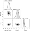 |
Fig. C.1. Posterior distributions for the black hole mass, mbh, the position angle, ϕ, and the flux scaling, Sscale. The sliding window is located at Δt = 1.7 h (30 frames) recovering the time range used for the synthetic data generation (see Text). |
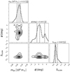 |
Fig. C.2. Posterior distributions for the black hole mass, mbh, the position angle, ϕ, and the flux scaling, Sscale, for the entire Kerr black hole a* = 0.94 data set. |
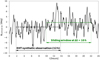 |
Fig. C.3. Variation of the image centroid position angle relative to the one from the sliding window used for the generation of the synthetic data (indicated by the black arrow). The mean centroid position angle for a second sliding window with a 10 h offset is indicated in green. |
All Tables
Effective antenna diameter d (for single telescopes this corresponds to the diameter of the dish) and system equivalent flux density (SEFD) used for the ground and space antennas (see Event Horizon Telescope Collaboration 2019b, for details).
Results of the cross-comparison of the synthetic images using the EHT 2017 and the advanced EHT configuration.
All Figures
|
Fig. 1. Top, panels A and B: GRRT images for a Kerr black hole with a* = 0.6 including scattering effects (diffractive and refractive scattering) for two selected times t = 12.6 h and t = 23.6 h (dash-dotted line in the bottom panel) at a frequency of 230 GHz. The average image for 24 h of observation is presented in panel C. Bottom: simulated total flux light curve at 230 GHz for 24 h of observations. A typical EHT observation with a duration of 12 h is indicated. |
| In the text | |
|
Fig. 2. Result of the orbit optimisation for 12 h of Sgr A* observations. Top row, from left to right: GRRT image (panel a), reconstructed image with interstellar scattering (including both diffractive and refractive scattering during the generation of the synthetic visibilities) using the EHT 2017 configuration convolved with 75% (red shading) of the nominal array resolution (light grey shading, panel b) and reconstructed image with interstellar scattering (including both diffractive and refractive scattering during the generation of the synthetic visibilities) using the space-EHT configuration convolved with 75% (red shading) of the nominal array resolution (light grey shading, panel c) for a dilaton black hole. Bottom row, from left to right: satellite orbit as seen from Sgr A* with orbital parameters and orbital period (panel d), satellite ground track (red lines for 12 h and grey ones for 24 h), ground array antennas (blue points, panel e), u − v sampling for the ground array (white points), and the baselines including the space antenna (red points, panel f). |
| In the text | |
|
Fig. 3. Comparison between synthetic data generation from a dynamical movie (blue lines) and from its static average frame (black lines) for the visibility amplitude (top) and closure phase (bottom) for Kerr black hole with a* = 0.6. |
| In the text | |
|
Fig. 4. Synthetic black hole images for Sgr A* for a Kerr black hole with a* = 0.94 (panels a–c), a Kerr black hole with a* = 0.6 (panels d–f), a non-rotating dilaton black hole (panels g–i), and for a stable, non-rotating boson star (panels j–l). From left to right and for all rows: GRRT image (panels a, d, g, j), dynamically reconstructed image with interstellar scattering (including both diffractive and refractive scattering during the generation of the synthetic visibilities) using the EHT 2017 configuration convolved with 75% (red shading) of the nominal beam size (light grey shading, panels b, e, h, k), and dynamically reconstructed image with interstellar scattering (including both diffractive and refractive scattering during the generation of the synthetic visibilities) using the space-EHT configuration convolved with 75% (red shading) of the nominal beam size (light grey shading, panels c, f, i, l). |
| In the text | |
|
Fig. 5. Illustration of the movie scoring scheme. From the GRRT data, via a sliding window, we selected a set of images from which a movie was created. From this movie, complex visibilities were generated and the χ2 between the synthetic data was computed while allowing the movie to rotate and vary in source size and flux density. The χ2 were minimised either using an evolutionary algorithm (EA) or an MCMC scheme. After the optimisation, the sliding window was advanced until the entire GRRT data set was sampled. |
| In the text | |
|
Fig. 6. Scoring result of the Kerr a* = 0.94 synthetic data to the Kerr a* = 0.94 model. The panels show from top to bottom the visibility amplitude, the closure phase, the calibrated gains, and the average image of the Kerr a* = 0.94 movie (GRRT left and convolved right). |
| In the text | |
|
Fig. 7. Results for the Kerr a* = 0.6 test. The panels show the distribution of the total |
| In the text | |
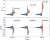 |
Fig. 8. Same as in Fig. 7, but for the Kerr a* = 0.94 test. |
| In the text | |
|
Fig. 9. Results for the Kerr a* = 0.6–dilaton black hole test with varying black hole mass. The panels show the distribution of the total |
| In the text | |
|
Fig. A.1. Reconstruction of a boson star image for Sgr A* (ground truth image in panel a) for the following three different satellite orbits: small orbit (second column), intermediate orbit (third column), and large orbit (fourth column). From top to bottom: reconstructed image convolved with 75% of the nominal array resolution, the uv-coverage (white: ground array baselines, red: space baselines), and the satellite orbit as seen from Sgr A*. |
| In the text | |
|
Fig. B.1. DSSIM and nCCC variation study. Top panel: ground truth images for Kerr a* = 0.6, Kerr a* = 0.94 and dilaton black holes (left most column) and convolved with decreasing beams (30 μas–1 μas). Middle panel: DSSIM and nCCC calculations using the average image of Kerr BH with a* = 0.6 as ground truth image. Bottom panel: DSSIM and nCCC calculations using the average image of Kerr BH with a* = 0.94 as ground truth image. |
| In the text | |
|
Fig. C.1. Posterior distributions for the black hole mass, mbh, the position angle, ϕ, and the flux scaling, Sscale. The sliding window is located at Δt = 1.7 h (30 frames) recovering the time range used for the synthetic data generation (see Text). |
| In the text | |
|
Fig. C.2. Posterior distributions for the black hole mass, mbh, the position angle, ϕ, and the flux scaling, Sscale, for the entire Kerr black hole a* = 0.94 data set. |
| In the text | |
|
Fig. C.3. Variation of the image centroid position angle relative to the one from the sliding window used for the generation of the synthetic data (indicated by the black arrow). The mean centroid position angle for a second sliding window with a 10 h offset is indicated in green. |
| In the text | |
Current usage metrics show cumulative count of Article Views (full-text article views including HTML views, PDF and ePub downloads, according to the available data) and Abstracts Views on Vision4Press platform.
Data correspond to usage on the plateform after 2015. The current usage metrics is available 48-96 hours after online publication and is updated daily on week days.
Initial download of the metrics may take a while.