| Issue |
A&A
Volume 648, April 2021
|
|
|---|---|---|
| Article Number | A118 | |
| Number of page(s) | 13 | |
| Section | Interstellar and circumstellar matter | |
| DOI | https://doi.org/10.1051/0004-6361/202140385 | |
| Published online | 26 April 2021 | |
Observations of 12.2 GHz methanol masers towards northern high-mass protostellar objects
Institute of Astronomy, Faculty of Physics, Astronomy and Informatics, Nicolaus Copernicus University,
Grudziadzka 5,
87-100
Torun, Poland
e-mail: This email address is being protected from spambots. You need JavaScript enabled to view it.
Received:
20
January
2021
Accepted:
12
March
2021
Abstract
Context. Class II methanol masers at 6.7 and 12.2 GHz occur close to high-mass young stellar objects (HMYSOs). When they are observed simultaneously, such studies may contribute to refining the characterisation of local physical conditions.
Aims. We aim to search for the 12.2 GHz methanol emission in 6.7 GHz methanol masers that might have gone undetected in previous surveys of northern sky HMYSOs, mainly due to their variability. Contemporaneous observations of both transitions are used to refine the flux density ratio and examine the physical parameters.
Methods. We observed a sample of 153 sites of 6.7 GHz methanol maser emission in the 12.2 GHz methanol line with the Torun 32 m radio telescope, using the newly built X-band receiver.
Results. The 12.2 GHz methanol maser emission was detected in 36 HMYSOs, with 4 of them detected for the first time. The 6.7–12.2 GHz flux density ratio for spectral features of the contemporaneously observed sources has a median value of 5.1, which is in agreement with earlier reports. The ratio differs significantly among the sources and for the periodic source G107.298+5.639 specifically, the ratio is weakly recurrent from cycle to cycle, but it generally reaches a minimum around the flare peak. This is consistent with the stochastic maser process, where small variations in the physical parameters along the maser path can significantly affect the ratio. A comparison of our data with historical results (from about ten years ago) implies significant (>50%) variability for about 47 and 14% at 12.2 and 6.7 GHz, respectively. This difference can be explained via the standard model of methanol masers.
Key words: masers / stars: massive / stars: formation / ISM: molecules / radio lines: ISM
© ESO 2021
1 Introduction
Masers play a significant role in the study of the interstellar medium. The methanol molecule has attracted much attention, from its first detection half a century ago (Barrett et al. 1971) to the present, given the multitude of observed transitions. One of the breakthroughs in the field came with the detection of the strongest, and most pervasive, lines at 12.2 (Batrla et al. 1987) and 6.7 GHz (Menten 1991), which provided powerful tools for identifying high-mass young stellar objects (HMYSOs) and exploring the physical conditions and gas kinematics of their surroundings. A number of new methanol transitions in the centimetre (Breen et al. 2019; MacLeod et al. 2019) and millimetre (Brogan et al. 2019) ranges have been discovered very recently in objects that have undergone major accretion events.
The 6.7 and 12.2 GHz lines are referred to as class II methanol maser transitions (Batrla et al. 1987; Menten 1991) that are characterised by radiative pumping (Cragg et al. 2005) and a close association with sources of strong radiation. They are usually found in the vicinity of HYMSOs, as revealed by several surveys at 6.7 GHz (e.g. Caswell et al. 1995b; Ellingsen et al. 1996; Pandian et al. 2007; Szymczak et al. 2012; Green et al. 2010; Breen et al. 2015). Several searches for the 12.2 GHz methanol maser emission were carried out prior to the discovery of the 6.7 GHz line, mainly towards OH maser sites (Norris et al. 1987; Koo et al. 1988; Kemball et al. 1988; Caswell et al. 1993; MacLeod et al. 1993). Thereafter, all the 12.2 GHz surveys were done towards the 6.7 GHz sources (Gaylard et al. 1994; Caswell et al. 1995a; Błaszkiewicz & Kus 2004; Breen et al. 2010, 2012a,b, 2014, 2015), as the 12.2 GHz line excitation conditions closely follow those at 6.7 GHz (Cragg et al. 2002). Almost all of these surveys did not cover the entire northern sky, thus, in this study, we attempt to supplement the observations with objects of the northern hemisphere.
No conclusive data is available on the variability patterns of the 12.2 GHz methanol masers. Little or no variability was noticed on a timescale of seven months in eight bright (>100 Jy) 12.2 GHz maser sources (McCutcheon et al. 1988), whereas in the other five bright sources, the emission varied internally by less than 15–20% over a four-year period with the exception of single weak features in two sources (MacLeod et al. 1993). In turn, Caswell et al. (1993) reported the 12.2 GHz flux density variations on a timescale of weeks and later found that at least a quarter of the features exhibit intensity variations larger than 10% on a timescale of 4 yr (Caswell et al. 1995a) suggesting that most quiescent 12.2 GHz masers are saturated. In this paper, we present the results of multi-epoch 12.2 GHz observations, along with a comparison to historical observations, for 153 sources. We include several contemporaneously monitored 6.7 GHz methanol maser counterparts.
2 Observations
Observations were carried out in the period from 2019 August to 2020 February using the Torun 32 m radio telescope. The telescope has a half-power beam width of about 3′ at 12.2 GHz and rms pointing errors of about 10′′. The adopted rest frequency was 12.178597 GHz (Müller et al. 2004). We used the newly built X-band receiver (Pazderski 2018), which is a dual-polarisation cooled receiver with amplifiers of typical noise temperatureof 5 K. Here, the system temperature was about 30 K. The antenna gain was estimated to be about 0.06 K Jy−1 from observations of calibrators DR21 and 3C123 adopting flux densities of 20.0 and 6.3 Jy, respectively (Ott et al. 1994). No gain elevation correction was applied; this can contribute less than 4% to the error budget of the flux density. The uncertainty in the flux density scale is about 15%.
The observations were made in frequency-switching mode. An autocorrelation spectrometer was configured to record 4096 channels either with 4 MHz or 8 MHz bandwidth for each circularly polarised signal yielding the channel spacing of 0.024 or 0.048 km s−1, respectively. The velocity extent of each observation is ±45 or ±90 km s−1 with respect to the local standard of rest. A typical 3σ noise level in the final spectra with the higher spectral resolution was 1.5 Jy. The stability of the system was regularly checked with observations of G188.946+0.886 that show no variability to a limit of 15% during our observing interval, while its 12.2 GHz spectrum shape remained almost unchanged after ⪞ 10 yr when observed by Breen et al. (2012a). Observations of G188.946+0.886 during the 2000–2008 revealed periodic (395±8 d) variability with relative amplitudes of 0.5 and 0.7 at 6.7 and 12.2 GHz, respectively, but periodic changes at 12.2 GHz were barely visible prior to 2005 (Goedhart et al. 2014, their Figs. 9 and 10). In the period from 2009 to 2013, the relative amplitude of periodic variations at 6.7 GHz decreased to about 0.2 (Szymczak et al. 2018), whereas our unpublished 6.7 GHz observations, carried out contemporaneously with the present 12.2 GHz survey, show a variability that is lower than 10% We argue that the variability of this object at 12 GHz does not exceed the uncertainty of our measurements. For selected sources, contemporaneous (≤ ±7 d) observations were carried out in the 6.7 GHz methanol transition following the procedure described in Szymczak et al. (2018).
We selected bright 6.7 GHz sources (Breen et al. 2015; Szymczak et al. 2012; Hu et al. 2016; Green et al. 2010) that are observable from the northern hemisphere and mostly with a declination of > 0° to avoid a degradation of the telescope sensitivity due to radio frequency interference from commercial satellites. The final sample consists of 153 sources.
3 Results
The 12.2 GHz maser emission was detected in 36 objects (Table 1), including four new sources. Figures 1 and A.1 present the spectra of newly detected and previously known sources, respectively. The list of non-detections is also given in Table A.1.
3.1 Newly detected 12.2 GHz sources
G50.035+0.582
This source has a single 12.2 GHz feature at −5.1 km s−1, with S12.2 = 1.1 Jy, which coincides with the strongest feature of the 6.7 GHz methanol maser (Szymczak et al. 2012; Breen et al. 2015). There was no 12.2 GHz maser emission detected in 2010 March with the 5σ sensitivity of 0.84 Jy (Breen et al. 2016). This implies a variability of ≥30% on a timescale of 9.5 yr.
G85.410+0.003
The 12.2 GHz spectrum is comprised of three features at −31.5, −29.5, and −28.6 km s−1. These are coincident with their 6.7 GHz maser counterparts, within 0.1 km s−1, observed in the same epoch. In instances where a single bright feature at V12.2 = −29.5 km s−1 was originally detected, we now report two features separated by 0.3 km s−1. A comparison with the Effelsberg 100 m spectrum taken on May 19, 2020 (Yen & Menten, priv. comm. at M2O1) implies significant changes in the profile shape and flux density of individual features by a factor of 2−3 over four months.
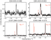 |
Fig. 1 Spectra of the newly detected 12.2 GHz methanol maser sources. Spectra of 6.7 GHz methanol masers (red) are also shown when taken on the same day, with exception of G183.348−0.575, where the interval between observations was 41 d. For comparison purposes, the scale of 6.7 GHz flux density was reduced by the factor given in the upper right corner. |
G107.298+5.639
The single velocity feature is matched in velocity to the strongest 6.7 GHz feature at −7.35 km s−1 (Olech et al. 2020) during all three observed cycles, which are discussed in detail in Sect. 3.2. Hereafter, G107.298+5.639 is referred to as G107.
G183.348−0.575
The 12.2 GHz maser emission consists of a single feature at −4.9 km s−1 with a peak flux density of 2.5 Jy, which coincides in velocity with the 6.7 GHz maser feature. There was no 12.2 GHz maser emission seen for the blueshifted component of the 6.7 GHz emission near −15 km s−1.
3.2 Case of G107
The 12.2 GHz maser emission follows periodic variations observed in the methanol 6.7 GHz and hydroxyl (1.665/1.667 GHz) maser lines (Szymczak et al. 2016; Olech et al. 2020). The upper panel in Fig. 2 presents the light curves of both methanol transitions. In order to estimate the parameters of flare profiles, we fitted an asymmetric power function (David et al. 1996; Szymczak et al. 2011), Gaussian function, and second-order polynomial to the 6.7 and 12.2 GHz data. The flare maximum and timescale of variability FWHM of the flare are listed in Table 2 for each transition and three cycles. For the asymmetric function fitting we get, in addition, the ratio of rise to decay time of the flare, which ranges from 0.8 to 1.1 and 0.7 to 0.9 for the 12.2 and 6.7 GHz lines, respectively. This suggests that the flare profile at 12.2 GHz is slightly more symmetric than the one at 6.7 GHz. The full width at half maximum (FWHM) values of 12.2 GHz flares (1.8−4.5 d) vary from cycle to cycle much more than those of 6.7 GHz flares (4.4−5.8 d), suggesting agreater variability of the 12.2 GHz emission.
There is a systematic delay between 6.7 and 12.2 GHz flare peaks (Table 2) for each of the three cycles (lower panel in Fig. 2). The average delay obtained from the results of the three fits is 0.9±0.3 d. The VLBI maps indicate that the 6.7 GHz emission near −7.35 km s−1 comes from clouds located ~150 au from the putative position of the central star (Olech et al. 2020). Thus, if the 6.7 and 12.2 GHz maser coexist, then the observed delay cannot be explained by a simple geometrical effect. We may speculate that the actual size of the region conducive for 6.7 GHz maser emission is more extended than it would be for 12.2 GHz maser emission and both maser regions may not coincide precisely. Further interferometric studies are needed to verify this possibility.
The lower part of Fig. 2 shows variations in the 6.7 to 12.2 GHz flux density ratio (R6∕12) over the cycles. There are significant differences in the temporal behaviour of R6∕12 over the flare profile from cycle to cycle. For the best sampled observations of the second cycle, with a peak around MJD 58 714, R6∕12 falls from 22 at flare onset to 10.4 at flare maximum and then increases to 32 as the flare decays. The average value of R6∕12 for the three cycles around the flare peaks is 8.1 which is very close to the median ratio reported in Caswell et al. (1995b) and Breen et al. (2014).
Detected 12.2 GHz methanol maser sources.
4 Comments on previously known sources
In this section, we provide commentary on our observational data with the aim of providing useful information on the 6.7 to 12.2 GHz flux density ratio. Taken together with results of previous surveys given in Table 1, it is possible to estimate thedegree and timescale of variability.
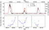 |
Fig. 2 Light curves of the −7.4 km s−1 methanol maser feature at 12.2 (black) and 6.7 GHz (red) for G107.298+5.639 (upper panel). Temporal changes in the 6.7–12.2 GHz flux density ratio are plotted (blue) (lower panel). The thick vertical error bars denote the flare maxima at 12.2 (black) and 6.7 GHz (red) calculated as the average value of the peak times obtained with the use of three methods (Table 2), whereas the thin horizontal error bars mark the corresponding standard errors. |
Flare parameters retrieved from the three model fitting.
G30.225−0.180
The 12.2 GHz maser spectrum detected in September and December 1992 by Caswell et al. (1995a) was composed of two features at V12.2 = 112.8 and 113.6 km s−1, with a peak flux density S12.2 ~ 2.8 and 1.2 Jy, respectively. Our observations reveal the spectrum of different shape with a peak flux density of S12.2 = 6.7 Jy at V12.2 = 113.3 km s−1. There was no emission found, with a 5σ sensitivity level of 1.8 Jy, in March 2010 (Breen et al. 2016). This implies significant variability on timescales of 9–27 yr. The emission at a velocity lower than 111 km s−1 (Fig. A.1) comes from another source, namely, G30.198−0.169 (Caswell et al. 1995a; Breen et al. 2016), which was detected in the beam sidelobe.
G32.744−0.075
A comparison of our observations with those in the literature suggests that the overall spectral profile of the 12.2 GHz maser emission has been unchanged over more than 40 yr (Caswell et al. 1993). The peak flux density of individual features differ by ≤40% on timescales of 9–27 yr (Caswell et al. 1993, 1995a; Breen et al. 2016), suggesting only modest variability.
G33.641−0.228
The brightest features in our spectrum have similar velocities to those reported in Breen et al. (2016), but their flux densities differ by a factor of 0.3–2.3. Furthermore, the emission at V12.2 = 58.8 km s−1 decreased by an order of magnitude as compared to that observed in 2002 by Błaszkiewicz & Kus (2004). This implies significant variability on timescales of 9–18 yr. The source also shows a variety of variability patterns in the 6.7 GHz methanol maser emission from short (2–5 d) flares, with a seven-fold rise within 24 hr (Fujisawa et al. 2012, 2014), up to quasi-periodic (>500 d) variations of low amplitude (Olech et al. 2019).
G35.132−0.744
The strongest feature at V12.2 = 31.2 km s−1 that was observed by Breen et al. (2016) increased by a factor of 2, whereas the feature at V12.2 = 29.7 km s−1 increased by one order of magnitude. This implies strong variability on a timescale of 9 yr.
G35.197−0.743
The spectrum observed in April 1988 (Caswell et al. 1993) is complex, with a prominent feature at V12.2 = 30.5 km s−1, with a peak flux of S12.2 = 44 Jy. The intensity of this feature decreased by ~30%, while the emission peak at V12.2 = 28.5 km s−1 increased by the same amount after ~4.5 yr (Caswell et al. 1995a). MacLeod et al. (1993) and Błaszkiewicz & Kus (2004) reported the spectrum similar to that observed in December 1992 by Caswell et al. (1995a), while the Breen et al. (2016) spectrum is similar to that presented in Caswell et al. (1993). Thus, from the data reported in the literature we infer a variability of 30–40% on a timescale of 4–20 yr. Our survey suggests that this level of variability remains on timescale of ≥30 yr for the redshifted emission (30.5 km s−1) but the feature at V12.2 = 28.2 km s−1 increased bya factor of 4 as compared to the spectrum from Breen et al. (2016).
G35.200−1.736
Norris et al. (1987) reported the spectrum, consisting of two features at V12.2 = 41.5 and 45.0 km s−1 with peak flux densities of S12.2 = 100 and 146 Jy, respectively. A similar spectrum was seen after 1–5 yr with slight (≤15%) decreases of peak intensity (Caswell et al. 1993, 1995a; Catarzi et al. 1993). Observations in 2002 (Błaszkiewicz & Kus 2004) and 2010 (Breen et al. 2016) displayed an ongoing complex spectrum with two prominent features but with the flux density of the strongest feature at V12.2 = 45.0 km s−1 decreasing to S12.2 = ~80 Jy in 2002 and S12.2 = 46 Jy in 2010. We report only a single feature with a peak of S12.2 = 12 Jy at V12.2 = 45.2 km s−1. We conclude that the 12.2 GHz line intensity declined by an order of magnitude within 32 yr.
G37.430+1.518
Our spectrum, with a single feature of S12.2 = 74 Jy at V12.2 = 41.3 km s−1, is very similar to that reported by Błaszkiewicz & Kus (2004) and Breen et al. (2016), implying a variability lower than 20% on a timescale of 17 yr. The emission observed 26 yr ago (Gaylard et al. 1994) was a factor of 6 weaker, suggesting significant variability on longer timescales.
G40.282−0.219
The three-feature spectrum is similar to that observed nine years ago (Breen et al. 2016) but the flux density of the primary feature at V12.2 = 74.3 km s−1 decreased by ~50%.
G42.034+0.190
We detected a weak and complex 12.2 GHz spectrum of similar shape to that shown in Breen et al. (2016). In general, the intensity of features increased by a factor of 1.8–4.5 after nine years.
G43.149+0.013
The 12.2 GHz spectrum consisted of a single feature at V12.2 = 13.6 km s−1. Its intensity declined by 35% over 26 yr (Caswell et al. 1995a; Breen et al. 2016).
G43.890−0.784
Little variability is visible in the two features at V12.2 = 47.4 and 51.8 km s−1 when compared to spectra from 2002 (Błaszkiewicz & Kus 2004) an 2010 (Breen et al. 2016). From our observations, it can be seen that the emission at V12.2 = 51.8 km s−1 decreased by a factor of 2. There was no emission detected at V12.2 = 47.7 km s−1, whereas a new feature appeared at V12.2 = 45.3 km s−1, indicating significant variability.
G49.043−1.079
Nine years ago, this 12.2 GHz source had a complex spectra (Breen et al. 2016). In our observations, the strongest feature they detected (S12.2 = 7.1 Jy at V12.2 = 37.4 km s−1) is now only ~1 Jy. This suggests strong variability on this timescale.
G49.416+0.326
The spectrum is similar to that presented in Breen et al. (2016), with little variability above the noise level.
G49.490−0.388
The spectrum is composed of the emission from G49.489−0.369 and G49.490−0.388 as part of the W51 complex. Batrla et al. (1987) discovered a single feature, with a peak flux density of S12.2 = 8 Jy at V12.2 ~ 56 km s−1, and a broad absorption feature (from 60 to 75 km s−1). Catarzi et al. (1993) observed a similar spectrum with a peak flux density of S12.2 = 20 Jy without absorption. Caswell et al. (1993, 1995a) also reported one feature with the peak flux density of S12.2 = 14 and 21 Jy, respectively with barely visible absorption. A simple spectrum with a single feature at V12.2 = 56.2 km s−1 with S12.2 = 13.8 Jy was also observed by Błaszkiewicz & Kus (2004). The flux density of this feature dropped to 4.5–5.5 Jy (in 2008 and 2010, Breen et al. 2016) and increased to ~10 Jy during our observations. This suggests that the emission towards G49.490−0.388 shows significant and complicated temporal changes. Features at velocity >56.6 km s−1 were also visible only in 2010 (Breen et al. 2016) that might suggest variability of G49.489−0.369. It is difficult, given our beam size, to distinguish unequivocally which spectral feature comes from which object; hence, the velocity ranges marked in Fig. A.1 are taken from Breen et al. (2016).
G49.599−0.249
The spectrum is almost the same as the one seen in Breen et al. (2016), with the exception of the 63.0 km s−1 feature, which decreased by a factor of 2 after 9 yr.
G59.783+0.065
The feature at V12.2 = 27.1 km s−1 declined from S12.2 = 15.8 Jy in 1992 (Caswell et al. 1995a) to S12.2 = 9.2 Jy in 2002 (Błaszkiewicz & Kus 2004) and S12.2 = 4.3 Jy during our observations. The second feature at V12.2 = 17.0 km s−1, with a peak flux of S12.2 = 4 Jy (Caswell et al. 1995a) increased by ~50% (Błaszkiewicz & Kus 2004) and decreased below our sensitivity limit of ~1 Jy.
G109.871+2.114
Observations made in 1990 (Catarzi et al. 1993), with a peak flux density of S12.2 = 128.8 Jy at V12.2 = −4.15 km s−1, found a similar spectral profile shape to that seen in 1987 (Koo et al. 1988), but with flux density that was a factor of ~2 lower. Błaszkiewicz & Kus (2004) revealed a similar profile but with peak flux densities that were a factor of 3 lower than Koo et al. (1988). We detected a complex spectrum with the emission from V12.2 = −5 to −1 km s−1 and a peak flux density of S12.2 = 45 Jy at V12.2 = −4.1 km s−1. Thus, the source is significantly variable, namely, by a factor of 7 on a timescale of ~30 yr.
G111.542+0.777
Batrla et al. (1987) discovered a double peaked spectrum, the brightest feature at V12.2 = −56.3 km s−1, with S12.2 ~200 Jy remained stable within 15% over 1–3 yr (Koo et al. 1988; Catarzi et al. 1993). The spectral shape was found to be unchanged in 2002 (Błaszkiewicz & Kus 2004) but the peak flux density decreased by a factor of 2. Here, we present a very different spectrum with several blended features from −62 to −55 km s−1. The feature at V12.2 = −56.3 km s−1 dimmed by a factor of 20 compared to that reported by Batrla et al. (1987), whereas the feature near V12.2 = −61.5 km s−1 increased by a factor of less than 2. This suggests strong variability on a timescale of ≥20 yr.
G188.946+0.886
The flux density of the strongest feature at V12.2 = 10.4 km s−1 increased by ~30% between 1987 and 1992 (Koo et al. 1988; Kemball et al. 1988; Caswell et al. 1993, 1995a; Catarzi et al. 1993). The profile of the spectrum significantly transformed in 2008 (Breen et al. 2012a) but the intensity remained unchanged within 10%.We found spectra similar to those reported in Breen et al. (2012a), and the peak flux of feature at V12.2 = 10.8 km s−1 increased by ~15%. More information on the variability of this object is provided in Sect. 2.
G192.600−0.048
A faint (0.5–0.6 Jy) feature at V12.2 = 3.6 km s−1 was detected in June and December 2008 (Breen et al. 2012a). Our observations revealed a complex spectrum with the strongest feature of S12.2 = 26 Jy at V12.2 = 5.8 km s−1. Significant change in the spectral profile and intensity is likely related to a significant outburst of a 6.7 GHz maser that occurred in mid-2015 (Moscadelli et al. 2017; Szymczak et al. 2018).
There is a group of 12.2 GHz masers that have gone undetected in the present survey (Table A.1) and 13 out of those 17 masers were observed with a 5σ sensitivity of 0.7–4.2 Jy, that is, lower than the peak flux densities at the time of their detection from the literature. We failed to detect, with 5σ sensitivity of 0.6–0.9 Jy, the following objects: G42.698−0.147, G45.467+0.053, G94.602−1.796, and G196.454−1.677, with a peak flux density of 1.2–12.3 Jy in earlier observations (Caswell et al. 1995a; Błaszkiewicz & Kus 2004; Breen et al. 2012a, 2016). These four sources may be variable on timescales smaller than 9–28 yr.
5 Discussion
5.1 Detection rate
The present observations of our sample of 153 6.7 GHz masers resulted in the detection of 36 12.2 GHz methanol maser sources, corresponding to a ~24% detection rate. This is about a factor of 2 lower than the overall detection rate of 43% in the Galactic longitude range of 290° ≤ l ≤ 60° (Breen et al. 2016). We compared our detection rate with the rates from Breen et al. (2016) as a function of 10° longitude bins. For the 30° −40°, 40° −50°, and 50° −60° longitude bins, our detection rates are lower by 20, 9, and 2%, respectively, than those reported in Breen et al. (2016). This confirms a significant lowering of our sensitivity for low declination sources as shown in Table A.1. The reason for this is a degradation of sensitivity due to interference from geostationary satellites or imperfect removal of some corrupted scans during the edition of spectra. The detection rate in the range of 70° ≤ l ≤ 90° decreases to ~16% and shows a statistically significant difference from that for the neighbouring range of 50° −60° (23.5%).
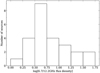 |
Fig. 3 Histogram of the 6.7–12.2 GHz peak flux density ratio. |
5.2 Flux density ratio
Our survey indicates that the flux density of individual features and integrated flux density of the 6.7 GHz maser sources are all greater thanthose of their 12.2 GHz counterparts. This is consistent with conclusions inferred from more comprehensive statistical analysis based on a large sample (Breen et al. 2011). In the following, we confine discussion to the flux density ratio R6∕12 for the spectral features with the same velocity in both transitions contemporaneously observed in order to exclude the possible effect of variability. There is strong observational evidence of spatial coincidence of the 6.7 and 12.2 GHz masers to within a few milliarcseconds, especially when the spectral profiles of both transitions are similar (Menten et al. 1992; Norris et al. 1993; Minier et al. 2000; Moscadelli et al. 2002). Thus, it is suggestive that the flux density comparison can be meaningful in the absence of high angular resolution maps. We found 70% of the detected 12.2 GHz methanol maser peaks are coincident in velocity with the 6.7 GHz maser peak.
For the 6.7 and 12.2 GHz spectra of nine sources taken within 7 days of each other, we performed Gaussian function fitsto obtain the velocity and flux density of feature peaks. For all features with the same peak velocity (± 0.1 km s−1) at both transitions, the flux density ratio, R6∕12, was determined (Table 3). The range of R6∕12 is 1.5 to 50.9, with a median value of 5.1 (Fig. 3). Our median is comparable to that determined by Caswell et al. (1995b). The analysis by Breen et al. (2011) of the statistical properties of 580 southern sources found a median peak-to-peak ratio of 4.3. Although their samples are more numerous, with little overlap with ours, the median ratios are similar. This suggests that each of these samples come from a similar population of HMYSOs.
There is a significant dispersion of R6∕12 for spectral features of some sources (e.g. G111.524+0.777, Table 3). Furthermore, our observations of G107 reveal that around the flare maxima, R6∕12 varies by up to 50% between two consecutive cycles. In addition, the temporal behaviour of R6∕12 is poorly repeated from cycle to cycle, even though a general trend remains, that is, the ratio reaches a minimum around the flare peak and is larger at the onset and final stages of the flare profile. This could be caused by variations in the physical conditions along the maser path length of 1016 cm (Moscadelli et al. 2002) for individual features on different timescales.
In G107, the maser intensity varies with a period of 34.4 days, perhaps due to changes of infrared emission (Olech et al. 2020); it is difficult to identify processes that can significantly change the gas density, molecule abundance, and kinetic temperature in the maser regions on such a short timescale. Since the heating and cooling times of dust grains are less than a few minutes and one day, respectively, for the optically thick case (van der Walt et al. 2009; Johnstone et al. 2013), rapid changes in the maser intensity may be related to variations in the dust temperature (Td). Timescales of gas heating and cooling are 2–3 orders of magnitude greater than those of dust grains (e.g. Johnstone et al. 2013); thus, the gas temperature variation can affect the maser emission in G107 on timescales of several months.
Numerical models of infrared pumping indicate that the 6.7 and 12.2 GHz methanol masers over a wide range of the gas densities and kinetic temperatures (Cragg et al. 2002, 2005), but there is a narrow range of dust temperature, Td, for which the flux ratio varies quite rapidly (Cragg et al. 2005, their Fig. 2). When the dust temperature increases from ~130 to ~170 K, R6∕12 decreases by a factor of 2 and vice versa. Therefore, the variations in Td qualitatively explain the observed change in the flux ratio during the flare of G107. However, it should be noted that the temporal behaviour of R6∕12 varies considerably from cycle to cycle, which is possibly the result of small variations in the physical conditions along the maser path and the degree of saturation (e.g. Breen et al. 2012b). High-cadence monitoring observations combined with a high angular resolution are required to resolve this discrepancy.
5.3 Variability
There are 24 detected sources in our sample that are in common with those observed by Breen et al. (2016) at 12.2 GHz and Breen et al. (2015) at 6.7 GHz, providing an opportunity to study variations on a timescale of ~10 yr. Seven objects with spectra comprised of multiple sources were not considered. In Fig. 4, we present the relative changes in the integrated flux density (Sint) between the two methanol maser transitions. In Fig. 5, the same analysis is presented, but for peak flux densities (Table A.2 shows exact values). Among 17 sources detected in two epochs, only two show Sint variability of more than 50% in both transitions, these are: G35.200−1.736 and G49.043−1.079. The first object dimmed by a factor of 14.5 and 8.2 at 12.2 GHz and
6.7 GHz, respectively. The second object weakened by a factor of 12.7 at 12.2 GHz but only a factor of 2.3at 6.7 GHz. G36.115+0.552 decreased by a factor of 2.2 at both lines. Two other objects (G45.804−0.356 and G49.265+0.311) varied by slightly more than 50% at 12.2 GHz but did not show significant variability at 6.7 GHz. For the subsample of 17 sources, the median value of relative changes in Sint is 1.19 and 1.33 for the 6.7 and 12.2 GHz lines, respectively. This general trend of a larger level of variability at 12.2 GHz than that at 6.7 GHz is more pronounced for the entire sample (Figs. 4 and 5) and is consistent with the standard model of methanol masers (Cragg et al. 2002, 2005). They demonstrated that both masers operate in a wide range of gas density (104 –108 cm−3), gas temperature (30–200 K), and dust temperature (130–350 K) but we can see that the slopes of the intensity versus these parameters are more flat at 6.7 GHz than at 12.2 GHz (Cragg et al. 2005). Thus, long-term (9–10 yr) changes of the parameters may lead to higher variability in the 12.2 GHz line. Since high angular resolution interferometric studies have revealed that the 6.7 and 12.2 GHz emission is spatially coincident, the effect of turbulence or changes in velocity coherence should be the same for both transitions. Table A.2 also presents comparison of the number of the features visible in 12.2 GHz spectra among the literature data (Breen et al. 2016) and this survey. Many of the features generally remain unchanged (±1 feature), with the exception of G35.200−1.736, for which a significant decrease of luminosity is observed in both 6.7 and 12.2 GHz lines.
6.7–12.2 GHz flux density ratio (R6∕12) for the Gaussian fitted features for all the sources contemporaneously observed at both maser transitions.
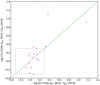 |
Fig. 4 Relative change in the integrated flux density, Sint at 6.7 and 12.2 GHz between 2010 (Breen et al. 2015, 2016) and 2019 (this survey). The square marks 50% level of variability. |
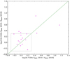 |
Fig. 5 Relative change in the peak flux density, Speak at 6.7 and 12.2 GHz between 2010 (Breen et al. 2015, 2016) and 2019 (this survey). The square marks 50% level of variability. Data used to create this graph is presented in Table A.2. |
6 Conclusions
We report that we detected 36 12.2 GHz methanol masers in our sample of 153, of which 4 are new detections, corresponding to detection rate of 24%.
Values of the 6.7–12.2 GHz flux density ratio for spectral features at the same velocity, when both transitions are observed contemporaneously, are within the range from 1.5 to 51. The median value of 5.1 is similar to that reported for other large samples of HYMSOs. This ratio in the periodic source G107.298+5.639 is smallest when the flare reaches its maximum, but it varies considerably from cycle to cycle. It decreases from its maximum value at the onset through its minimum at the peak of the flare and then increases during the decay phase of the flare. This temporal behaviour appears to be consistent with the standard model of methanol masers when the dust temperature varies in the narrow range of 130–170 K.
A minority (14%) of the objects that we observed show strong (>50%) variability at 6.7 GHz over a timescale of 9–10 yr, but at 12.2 GHz, nearly half of the observed sources experienced strong variability. These results appear to be compatible with maser model predictions.
Acknowledgements
We thank the staff of the 32 m telescope for assistance with the observations. We also thank the referee for the careful reading of the manuscript and recommendations. The research has made use of the SIMBAD data base, operated at CDS (Strasbourg, France), as well as NASA’s Astrophysics Data System Bibliographic Services. The 32 m telescope is operated by the Institute of Astronomy, Nicolaus Copernicus University and supported by the Polish Ministry of Science and Higher Education SpUB grant.
Appendix A Additional material
Targets towards which no 12.2 GHz emission was detected in the survey.
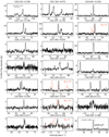 |
Fig. A.1 Spectra of 12.2 (black) and 6.7 GHz (red) methanol maser lines for previously known sources. The 6.7 GHz spectrum is shown only if taken contemporaneously with that at 12.2 GHz. The flux density of 6.7 GHz line is scaled by the factor given in the upper right corner. |
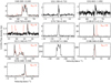 |
Fig. A.1 continued. |
References
- Barrett, A. H., Schwartz, P. R., & Waters, J. W. 1971, ApJ, 168, L101 [Google Scholar]
- Batrla, W., Matthews, H. E., Menten, K. M., & Walmsley, C. M. 1987, Nature, 326, 49 [Google Scholar]
- Błaszkiewicz, L., & Kus, A. J. 2004, A&A, 413, 233 [NASA ADS] [CrossRef] [EDP Sciences] [Google Scholar]
- Breen, S. L., Ellingsen, S. P., Caswell, J. L., & Lewis, B. E. 2010, MNRAS, 401, 2219 [Google Scholar]
- Breen, S. L., Ellingsen, S. P., Caswell, J. L., et al. 2011, ApJ, 733, 80 [Google Scholar]
- Breen, S. L., Ellingsen, S. P., Caswell, J. L., et al. 2012a, MNRAS, 426, 2189 [Google Scholar]
- Breen, S. L., Ellingsen, S. P., Caswell, J. L., et al. 2012b, MNRAS, 421, 1703 [Google Scholar]
- Breen, S. L., Ellingsen, S. P., Caswell, J. L., et al. 2014, MNRAS, 438, 3368 [Google Scholar]
- Breen, S. L., Fuller, G. A., Caswell, J. L., et al. 2015, MNRAS, 450, 4109 [Google Scholar]
- Breen, S. L., Ellingsen, S. P., Caswell, J. L., et al. 2016, MNRAS, 459, 4066 [Google Scholar]
- Breen, S. L., Sobolev, A. M., Kaczmarek, J. F., et al. 2019, ApJ, 876, L25 [CrossRef] [Google Scholar]
- Brogan, C. L., Hunter, T. R., Towner, A. P. M., et al. 2019, ApJ, 881, L39 [CrossRef] [Google Scholar]
- Caswell, J. L., Gardner, F. F., Norris, R. P., et al. 1993, MNRAS, 260, 425 [Google Scholar]
- Caswell, J. L., Vaile, R. A., Ellingsen, S. P., & Norris, R. P. 1995a, MNRAS, 274, 1126 [NASA ADS] [Google Scholar]
- Caswell, J. L., Vaile, R. A., Ellingsen, S. P., Whiteoak, J. B., & Norris, R. P. 1995b, MNRAS, 272, 96 [Google Scholar]
- Catarzi, M., Moscadelli, L., & Panella, D. 1993, A&AS, 98, 127 [NASA ADS] [Google Scholar]
- Cragg, D. M., Sobolev, A. M., & Godfrey, P. D. 2002, MNRAS, 331, 521 [Google Scholar]
- Cragg, D. M., Sobolev, A. M., & Godfrey, P. D. 2005, MNRAS, 360, 533 [NASA ADS] [CrossRef] [Google Scholar]
- David, P., Etoka, S., & Le Squeren, A. M. 1996, A&AS, 115, 387 [Google Scholar]
- Ellingsen, S. P., von Bibra, M. L., McCulloch, P. M., et al. 1996, MNRAS, 280, 378 [Google Scholar]
- Fujisawa, K., Sugiyama, K., Aoki, N., et al. 2012, PASJ, 64, 17 [Google Scholar]
- Fujisawa, K., Aoki, N., Nagadomi, Y., et al. 2014, PASJ, 66, 109 [Google Scholar]
- Gaylard, M. J., MacLeod, G. C., & van der Walt, D. J. 1994, MNRAS, 269, 257 [Google Scholar]
- Goedhart, S., Maswanganye, J. P., Gaylard, M. J., & van der Walt, D. J. 2014, MNRAS, 437, 1808 [Google Scholar]
- Green, J. A., Caswell, J. L., Fuller, G. A., et al. 2010, MNRAS, 409, 913 [Google Scholar]
- Hu, B., Menten, K. M., Wu, Y., et al. 2016, ApJ, 833, 18 [NASA ADS] [CrossRef] [Google Scholar]
- Johnstone, D., Hendricks, B., Herczeg, G. J., & Bruderer, S. 2013, ApJ, 765, 133 [NASA ADS] [CrossRef] [Google Scholar]
- Kemball, A. J., Gaylard, M. J., & Nicolson, G. D. 1988, ApJ, 331, L37 [Google Scholar]
- Koo, B.-C., Williams, D. R. D., Heiles, C., & Backer, D. C. 1988, ApJ, 326, 931 [Google Scholar]
- MacLeod, G. C., Gaylard, M. J., & Kemball, A. J. 1993, MNRAS, 262, 343 [Google Scholar]
- MacLeod, G. C., Sugiyama, K., Hunter, T. R., et al. 2019, MNRAS, 489, 3981 [CrossRef] [Google Scholar]
- McCutcheon, W. H., Wellington, K. J., Norris, R. P., et al. 1988, ApJ, 333, L79 [Google Scholar]
- Menten, K. M. 1991, ApJ, 380, L75 [NASA ADS] [CrossRef] [Google Scholar]
- Menten, K. M., Reid, M. J., Pratap, P., Moran, J. M., & Wilson, T. L. 1992, ApJ, 401, L39 [Google Scholar]
- Minier, V., Booth, R. S., & Conway, J. E. 2000, A&A, 362, 1093 [NASA ADS] [Google Scholar]
- Moscadelli, L., & Catarzi, M. 1996, A&AS, 116, 211 [NASA ADS] [CrossRef] [EDP Sciences] [Google Scholar]
- Moscadelli, L., Menten, K. M., Walmsley, C. M., & Reid, M. J. 2002, ApJ, 564, 813 [Google Scholar]
- Moscadelli, L., Sanna, A., Goddi, C., et al. 2017, A&A, 600, L8 [NASA ADS] [CrossRef] [EDP Sciences] [Google Scholar]
- Müller, H. S. P., Menten, K. M., & Mäder, H. 2004, A&A, 428, 1019 [NASA ADS] [CrossRef] [EDP Sciences] [Google Scholar]
- Norris, R. P., Caswell, J. L., Gardner, F. F., & Wellington, K. J. 1987, ApJ, 321, L159 [Google Scholar]
- Norris, R. P., Whiteoak, J. B., Caswell, J. L., Wieringa, M. H., & Gough, R. G. 1993, ApJ, 412, 222 [Google Scholar]
- Olech, M., Szymczak, M., Wolak, P., Sarniak, R., & Bartkiewicz, A. 2019, MNRAS, 486, 1236 [Google Scholar]
- Olech, M., Szymczak, M., Wolak, P., Gérard, E., & Bartkiewicz, A. 2020, A&A, 634, A41 [Google Scholar]
- Ott, M., Witzel, A., Quirrenbach, A., et al. 1994, A&A, 284, 331 [NASA ADS] [Google Scholar]
- Pandian, J. D., Goldsmith, P. F., & Deshpande, A. A. 2007, ApJ, 656, 255 [Google Scholar]
- Pazderski, E. 2018, Balt. URSI Symp., 33 [Google Scholar]
- Szymczak, M., Wolak, P., Bartkiewicz, A., & van Langevelde, H. J. 2011, A&A, 531, L3 [NASA ADS] [CrossRef] [EDP Sciences] [Google Scholar]
- Szymczak, M., Wolak, P., Bartkiewicz, A., & Borkowski, K. M. 2012, Astron. Nachr., 333, 634 [Google Scholar]
- Szymczak, M., Olech, M., Wolak, P., Bartkiewicz, A., & Gawroński, M. 2016, MNRAS, 459, L56 [Google Scholar]
- Szymczak, M., Olech, M., Sarniak, R., Wolak, P., & Bartkiewicz, A. 2018, MNRAS, 474, 219 [NASA ADS] [CrossRef] [Google Scholar]
- van der Walt, D. J., Goedhart, S., & Gaylard, M. J. 2009, MNRAS, 398, 961 [Google Scholar]
All Tables
6.7–12.2 GHz flux density ratio (R6∕12) for the Gaussian fitted features for all the sources contemporaneously observed at both maser transitions.
All Figures
|
Fig. 1 Spectra of the newly detected 12.2 GHz methanol maser sources. Spectra of 6.7 GHz methanol masers (red) are also shown when taken on the same day, with exception of G183.348−0.575, where the interval between observations was 41 d. For comparison purposes, the scale of 6.7 GHz flux density was reduced by the factor given in the upper right corner. |
| In the text | |
|
Fig. 2 Light curves of the −7.4 km s−1 methanol maser feature at 12.2 (black) and 6.7 GHz (red) for G107.298+5.639 (upper panel). Temporal changes in the 6.7–12.2 GHz flux density ratio are plotted (blue) (lower panel). The thick vertical error bars denote the flare maxima at 12.2 (black) and 6.7 GHz (red) calculated as the average value of the peak times obtained with the use of three methods (Table 2), whereas the thin horizontal error bars mark the corresponding standard errors. |
| In the text | |
|
Fig. 3 Histogram of the 6.7–12.2 GHz peak flux density ratio. |
| In the text | |
|
Fig. 4 Relative change in the integrated flux density, Sint at 6.7 and 12.2 GHz between 2010 (Breen et al. 2015, 2016) and 2019 (this survey). The square marks 50% level of variability. |
| In the text | |
|
Fig. 5 Relative change in the peak flux density, Speak at 6.7 and 12.2 GHz between 2010 (Breen et al. 2015, 2016) and 2019 (this survey). The square marks 50% level of variability. Data used to create this graph is presented in Table A.2. |
| In the text | |
|
Fig. A.1 Spectra of 12.2 (black) and 6.7 GHz (red) methanol maser lines for previously known sources. The 6.7 GHz spectrum is shown only if taken contemporaneously with that at 12.2 GHz. The flux density of 6.7 GHz line is scaled by the factor given in the upper right corner. |
| In the text | |
|
Fig. A.1 continued. |
| In the text | |
Current usage metrics show cumulative count of Article Views (full-text article views including HTML views, PDF and ePub downloads, according to the available data) and Abstracts Views on Vision4Press platform.
Data correspond to usage on the plateform after 2015. The current usage metrics is available 48-96 hours after online publication and is updated daily on week days.
Initial download of the metrics may take a while.