| Issue |
A&A
Volume 648, April 2021
|
|
|---|---|---|
| Article Number | A16 | |
| Number of page(s) | 13 | |
| Section | Stellar atmospheres | |
| DOI | https://doi.org/10.1051/0004-6361/202039761 | |
| Published online | 07 April 2021 | |
Gemini/Phoenix H-band analysis of the globular cluster AL 3★
1
Universidade de São Paulo, IAG, Rua do Matão 1226, Cidade Universitária,
São Paulo
05508-900, Brazil
e-mail: This email address is being protected from spambots. You need JavaScript enabled to view it.
2
UK Astronomy Technology Centre, Royal Observatory, Blackford Hill,
Edinburgh,
EH9 3HJ, UK
3
IfA, University of Edinburgh, Royal Observatory, Blackford Hill,
Edinburgh,
EH9 3HJ, UK
4
Instituto de Astronomía, Universidad Nacional Autónoma de México, A. P. 106,
22800, Ensenada, B. C., Mexico
5
Instituto de Astrofísica, Pontificia Universidad Católica de Chile,
Av. Vicuña Mackenna 4860, Santiago, Chile
6
Millennium Institute of Astrophysics,
Av. Vicuña Mackenna 4860,
782-0436 Macul, Santiago, Chile
7
Departamento de Ciencias Fisicas, Facultad de Ciencias Exactas, Universidad Andrés Bello,
Av. Fernandez Concha 700,
Las Condes, Santiago, Chile
8
Vatican Observatory, 00120 Vatican City State, Italy
9
Instituto de Alta Investigación, Sede Esmeralda, Universidad de Tarapacá,
Av. Luis Emilio Recabarren 2477, Iquique, Chile
10
Università di Padova, Dipartimento di Fisica e Astronomia, Vicolo dell’Osservatorio 2,
35122
Padova, Italy
11
INAF-Osservatorio Astronomico di Padova,
Vicolo dell’Osservatorio 5,
35122
Padova, Italy
12
Universidade Federal do Rio Grande do Sul, Departamento de Astronomia, 15051,
Porto Alegre
91501-970, Brazil
Received:
26
October
2020
Accepted:
9
February
2021
Abstract
Context. The globular cluster AL 3 is old and located in the inner bulge. Three individual stars were observed with the Phoenix spectrograph at the Gemini South telescope. The wavelength region contains prominent lines of CN, OH, and CO, allowing the derivation of C, N, and O abundances of cool stars.
Aims. We aim to derive C, N, O abundances of three stars in the bulge globular cluster AL 3, and additionally in stars of NGC 6558 and HP 1. The spectra of AL 3 allows us to derive the cluster’s radial velocity.
Methods. For AL 3, we applied a new code to analyse its colour-magnitude diagram. Synthetic spectra were computed and compared to observed spectra for the three clusters.
Results. We present a detailed identification of lines in the spectral region centred at 15 555 Å, covering the wavelength range 15 525–15 590 Å. C, N, and O abundances are tentatively derived for the sample stars.
Key words: stars: abundances / stars: atmospheres / Galaxy: bulge / globular clusters: individual: NGC 6558 / globular clusters: individual: AL 3 / globular clusters: individual: HP 1
Observations collected at the Gemini Observatory, Proposals GS-2006A-C9 and GS-2008A-Q-23-5, and at the European Southern Observatory (ESO), Proposal 64L-0212(A).
© ESO 2021
1 Introduction
The globular clusters AL 3, NGC 6558, and HP 1 share the characteristics of having a metallicity of [Fe/H] ~−1.0 and of being located in the Galactic bulge. They are old and could represent the earliest stellar populations in the Galaxy (Ortolani et al. 2006; Barbuy et al. 2018a; Kerber et al. 2019).
The star cluster AL 3 was discovered by Andrews & Lindsay (1967) and was also cataloged as BH 261 by van den Bergh & Hagen (1975), reported as a faint open cluster. It is reported in the ESO/Uppsala catalogue (Lauberts 1982) as ESO 456-SC78. Ortolani et al. (2006) showed that the star cluster shows B, V, I colour-magnitude diagrams (CMD) typical of a globular cluster. It is centred at J2000 α = 18h14m06.6s, δ = −28° 38′06″, with Galactic coordinates l = 3.36°, b = −5.27°, and located at 6. °25 and 2 kpc from the Galactic centre, hence in the inner bulge volume. The cluster has a depleted red giant branch (RGB), similarly to low-mass Palomar clusters, indicating it to have been stripped along its lifetime. This cluster has not been further observed so far.
The NGC 6558 cluster is located in a window, identified by Blanco (1988), with equatorial coordinates (J2000) α = 18h 10m 18.4s, δ = −31°45′49″ and Galactic coordinates l = 0.201°, b = −6.025°. It was analysed in terms of CMD by Rich et al. (1998). Rossi (2015) obtained a proper-motion-cleaned CMD and presented a proper motion analysis, from which a study of its orbits was given in Pérez-Villegas et al. (2018) and revised in Pérez-Villegas et al. (2020) using results from Baumgardt et al. (2019).
The globular cluster Cl Haute-Provence 1 or HP 1, also designated BH 229 and ESO 455-SC11, was discovered by Dufay et al. (1954). It is located at J2000 α = 17h31m05.2s, δ = −29° 58′ 54″, with Galactic coordinates l = 357.42°, b = 2.12°.
In the present work, we studied individual stars of these clusters in a limited region of the spectrum in the H-band corresponding to the wavelength region of the Phoenix spectrograph at the Gemini South telescope, centred at 15 555 Å, and covering 15 520–15 590 Å, with a high spectral resolution of R ~75 000. This region was chosen for containing prominent lines of CN, CO, and OH.
In Sect. 2, we examine the list of atomic and molecular lines in the region. In Sect. 4, the observationsare described. In Sect. 5, the CMD is analysed. In Sect. 6, the stellar parameters are given. In Sect. 7, the C, N, O abundances are derived. Conclusions are drawn in Sect. 7.
2 Spectroscopy in the H-band: atomic and molecular lines
The H-band will be intensely observed in the near future, given the new instruments placing emphasis on the near-infrared region, such as the James Webb Space Telescope (JWST), and new spectrographs on ground-based telescopes such as MOONS at VLT (presently CRIRES at VLT is available) and MOSAIC at ELT. The project APOGEE (Apache Point Observatory Galactic Evolution Experiment), with observations at a resolution of R ~ 22 000 carried out at the 2.5-m Sloan Foundation Telescope at the Apache Point Observatory in New Mexico (APOGEE-2N), and the 2.5-m du Pont Telescope at Las Campanas Observatory in Chile (APOGEE-2S), as described in Majewski et al. (2017) has shown the power of the H-band.
Given the short wavelength range covering only 70 Å of the Phoenix spectrograph, we faced the challenge of identifying the lines in moderately metal-poor stars of the Galactic bulge, for which only a few lines are available. Because the available lamps did not include lines in this region, and experience proved that sky lines yielded a better wavelength calibration, and given the short wavelength range, it is not straightforward to identify the lines.
For this reason, we proceeded to a line identification, in the spectra of the reference stars Arcturus and μ Leo, and created a shortened version of a line list, containing only detectable lines.
Meléndez & Barbuy (1999, hereafter MB99) worked on a list of atomic lines in the J and H bands. The list of lines mostly corresponded to the detectable lines. That previous line list needed to be largely completed. Upon checking the lines detectable in the wavelength range 15 520–16 000 Å, this was done by verifying the line lists from APOGEE (Shetrone et al. 2015) and VALD (Piskunov et al. 1995, Ryabchikova et al. 2015). We note that astrophysical oscillator log gf strengths were applied to the APOGEE line list, and these should be suitable for abundance derivation. Through a line-by-line check of its detectability in the Arcturus spectrum, we identified lines of Mg I, Si I, Ca I, Ti I, Mn I, and Ni I, and we were not able to find detectable lines from the species C I, O I, Sc I, V I, Cr I, Co I, Cu I, Y I, and Y II. The spectra computed including all lines of all these elements are entirely equivalent to the one computed with the shortened line list, therefore to ensure practicality when identifying which lines really contribute to a feature, we created a table containing the detectable lines only. In this table, available upon request, we report the oscillator strengths from MB99, APOGEE, VALD, and adopted values, where in order of preference we adopted NIST and MB99.
Molecular electronic transition lines of CN A2 Π-X2Σ, and vibration-rotation CO X1Σ+, OH X2Π lines were included in the synthetic spectra calculations. The line lists for CN were made available by S. P. Davis, the CO line lists were adopted from Goorvitch (1994), and the OH line list was made available by S. P. Davis and A. Goldman (Goldman et al. 1998). For more details on CN, CO, and OH molecular lines, we refer the reader to Meléndez & Barbuy (1999, 2002) and Meléndez et al. (2001). TiO ϕ-system b1 Π-d1 Σ lines are also present in the region. The line list by Jorgensen (1994) is included in the calculations as described in Schiavon & Barbuy (1999) and Barbuy et al. (2018a). The adopted dissociation potential of OH is 4.392 eV, D0 = 11.092 eV for CO and D0 = 7.65 eV for CN (Huber & Herzberg 1979). The PFANT code employed here for calculations of synthetic spectra is described in Barbuy et al. (2018b), and it is available together with the atomic and molecular line lists1.
We identified the lines in the reference stars Arcturus and μ Leo. For the reference star Arcturus, the spectrum atlas from Hinkle et al. (1995) is used, and for the metal-rich reference giant star μ Leo, APOGEE spectra are used, and their studies will be presented elsewhere.
The adopted stellar parameters for Arcturus and μ Leo are from Meléndez et al. (2003) and Lecureur et al. (2007), and they are reported in Sect. 5.
Log book of observations.
3 Observations
The spectra of red giant stars of the bulge globular clusters NGC 6558, AL 3, and HP 1 were observed with the Phoenix spectrograph installed on the 8m Gemini South telescope. The program was tri-national from Brazil (PI: B. Barbuy), Chile (PI: M. Zoccali),and Australia (PI: J. Meléndez).
The final suitable spectra include three stars of AL 3, two stars of NGC 6558, and one star of HP 1, centred at 1.555 μm in the H band. Another three stars in NGC 6558, and three in HP 1 were also observed; however, these showed a low signal-to-noise (S/N), due to clouds or high airmass. The log of observations is provided in Table 1.
This is the first spectroscopic work on AL 3, except for Gaia data (Gaia Collaboration 2021). In Fig. 1, a 3 min B exposure of AL 3 is shown for a field extraction of 3.3′ × 3.3′ (510 × 510 pixels). The sample stars of AL 3 are identified in the chart. Charts and identifications of the observed stars in NGC 6558 and HP 1 are given in Barbuy et al. (2007, 2018c) and Barbuy et al. (2006, 2016), respectively.
3.1 Gaia cross-check
In order to verify the corresponding membership probability of observed stars in AL 3, we performed the cross-match with Gaia Early Data Release 3 (EDR3; Gaia Collaboration 2021). We selected stars within 20′ from the cluster centre and used the renormalised unit weight error (RUWE) ≤ 2.4 to ensure the kinematics precision and the minimum match separation.
Having the high-precision EDR3 proper motions ( = μα cosδ and μδ), we obtain the mean proper motions for the cluster of
  mas yr−1 and μδ = − 3.54 ± 0.04 mas yr−1. These values are compatible with those given in Baumgardt et al. (2019). We also computed the Gaussian membership probability distribution of AL 3. We found that the stars AL3-6 and AL3-7 have membershipprobabilities of 100%. Finally, the star AL3-3 has a relatively low membership probability of ~ 60%, but still, it could be considered a member. Therefore, all three observed stars are probable members of AL 3. Table 2 provides the Gaia EDR3 cross-match and the membership probabilities.
Gaia magnitudes, proper motions and membership probability.
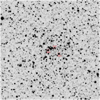 |
Fig. 1 AL 3: 3 min B image with the three sample stars identified. Extraction of 3′ × 3′. North is up and east is left. |
3.2 Radial velocity of AL 3
We were able to derive radial velocities for the sample stars. We used the low S/N individual observations of each star (S∕N ~ 10.0) combined to increase the signal-to-noise to S∕N ~18.0, and S∕N ~22.0 for AL3-3 and AL3-7, respectively. Due to the stacking process, the most prominent features identified are FeI 15 534.26, OH 15 542.10, TiI 15 543.758, TiO/NiI 15 55.25 blend, CN 15 555.25, and FeI 15 591.49. We also used the OH sky lines, as listed in Table 2 by Meléndez et al. (2003). These features were used for AL3-3, giving a radial velocity of −67.65 ± 3.65 kms−1. In the combined spectrum of AL3-7, the same features result in a radial velocity of −68.93 ± 4.83 kms−1. The corresponding heliocentric velocities of −57.29 km s−1 and −58 57 km s−1 lead to a final mean heliocentric velocity of −57.93 km s−1 ± 4.28 for AL 3. Figures 2 and 3 show the line identification and radial velocity derivation.
The star AL3-6 shows a very noisy spectrum, and we verified that it was observed under a high airmass of over 1.3, which also explains that it is plagued with telluric features. For AL3-6, we obtained a different heliocentric radial velocity, as shown in Fig. 4, of −29.57 ± 5.85 km s−1, compatible with the value given by Baumgardt et al. (2019) of −29.38 ± 0.60 km s−1.
The derived radial velocity is of crucial importance for the computation of the cluster’s orbits – see Sect. 5. However, we obtained two different figures:  = −57.93 and −29.57 km s−1. In Fig. 4, we show the spectrum of AL3-6 compared with that of AL3-7. Therefore, we obtained two different radial velocities for AL 3, and consequently we considered both of them for the calculation of orbits. Since we had already computed the orbits for the lower value (from Baumgardt et al. 2019), we show the orbits for the higher value here. Clearly, new observations of these stars in a more extended wavelength range and with a higher S/N would be of great interest.
4 Colour-magnitude diagram of AL 3
Ortolani et al. (2006) presented B, V, and Cousins I images of AL 3, observed on 2000 March 6 using the 1.54m Danish telescope at the European Southern Observatory (ESO) at La Silla. They derived a reddening of E(B–V) = 0.36 ± 0.03 and a distance of 6.0 ± 0.5 kpc, based on the magnitude of the horizontal branch (HB) of AL 3, and suggested a metallicity of [Fe/H] = − 1.3 ± 0.3 from a comparison of the CMD with the mean locus of the cluster M5.
Rossi (2015) described the observations with EFOSC at the NTT (ESO), La Silla in May 2012. They reported a distance of ~6.5 kpc, in agreement with (Harris 1996, edition of 2010). Pérez-Villegas et al. (2020) adopted both distances of 6.0 and 6.5 kpc and the radial velocity from Baumgardt et al. (2019) for the calculation of orbits.
We carried out the isochrone fitting using the SIRIUS code (Souza et al. 2020) on the same AL 3 data presented in Ortolani et al. (2006). The metallicity was limited by using a Gaussian prior with the value of Ortolani et al. (2006). We adopted the Dartmouth Stellar Evolution Database (DSED – Dotter et al. 2008), with [α/Fe] = 0.4 and primordial helium. The asymptotic giant branch (AGB) is also shown, based on BaSTI isochrones (Pietrinferni et al. 2006), since they are not available in DSED. The result is in very good agreement with results from Ortolani et al. (2006) within 1 − σ. We obtain a reddening of E(B − V) = 0.38 ± 0.04, a distance of d⊙ = 6.0 ± 0.6 kpc, and a metallicity of [Fe/H] = − 1.34 ± 0.18. Our age determination indicates an old age of  Gyr, indicating that AL 3 is another relic fossil. It is important to stress that our distance of 6.0 kpc is also in agreement, within 1 − σ, with the value of 6.5 kpc from Harris (1996), Rossi (2015), and Baumgardt et al. (2019).
Finally, we note that the dispersion of the data could be due to differential reddening, together with contamination and blends. The reddening of AL 3 is relatively high, and the differential reddening is certainly an issue, as it is in other bulge globular clusters with similar reddening. We expect an amount of about 20% of differential reddening. In principle it can be corrected, but the standard procedures for differential reddening correction in this cluster cannot be applied due to the few bona fide reference stars in the CMDs.
Figure 5 shows the solution of isochrone fitting. The solid blue line represents the median solution, while the shaded regions indicate the solutions within 1 − σ. The red stars are the three sample stars. Finally, Fig. A.1 exhibits the corner plots showing the (anti)correlations between the parameters.
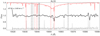 |
Fig. 2 AL 3-3: radial velocity derivation. The solid black line is the observed spectrum, the solid grey line is the noise spectrum, the solid red line is the synthetic spectrum, the dashed red lines are those used to derive the radial velocity, and the dashed black lines are the OH sky lines. |
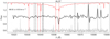 |
Fig. 3 AL 3-7: radial velocity derivation. The solid black line is the observed spectrum, the solid grey line is the noise spectrum, the solid red line is the synthetic spectrum, the dashed red lines are those used to derive the radial velocity, and the dashed black lines are the OH sky lines. |
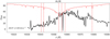 |
Fig. 4 AL 3-6: radial velocity derivation. The solid black line is the observed spectrum, the solid grey line is the spectrum of star AL3-7, the dashed red lines are those used to derive the radial velocity, and the dashed black lines are the OH sky lines. |
5 Stellar parameters
5.1 NGC6558 and HP 1
Individual stars of NGC 6558 were analysed with high-resolution spectroscopy by Barbuy et al. (2007, 2018c) and with moderate-resolution spectroscopy by Dias et al. (2015). The stars NGC 6558-42 and NGC 6558-64 are studied here.
Similar studies of HP 1 were carried out in Barbuy et al. (2006, 2016) and Dias et al. (2016). In the 2006 article, the bright red giants were labelled with numbers 1 to 6, for the purpose of identifying them in the cluster chart. In 2016, we adopted the identification numbers corresponding to the photometric reductions relative to observations obtained at the New Technology Telescope (NTT) at ESO, in 1994, as described in Ortolani et al. (1997). HP1-4 and HP1-5 are stars 2115 and 2939 in Barbuy et al. (2016). HP1-2 is the same as in Barbuy et al. (2016). In our study, we only analysed HP1-5.
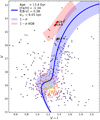 |
Fig. 5 AL 3 V vs. V − I CMD. The black dots are the stars within 120 pixels from the cluster centre (see Ortolani et al. 2006). The red stars are the observed stars of the present work. The solid blue line represents the median solution of the isochrone fitting, while the blue region reveals the solutions within 1 − σ from Dartmouth isochrones, and the rose region corresponds to BaSTI solutions for the AGB. |
5.2 AL 3
The magnitudes and colours as follows are indicated in Table 3: B, V from Ortolani et al. (2006), V, I from Rossi (2015), JHK from the 2MASS catalogue (Skrutskie et al. 2006)2, and JHK from the VVV survey (VVV Collaboration 2012)3.
Effective temperatures were initially derived from B−V, V − I, V − K, and J− K using the colour-temperature calibrations of Alonso et al. (1999). V,I Cousins were transformed to V,I Johnson using (V −I)C = 0.778(V −I)J (Bessell 1979). The J, H, KS magnitudes and colours were transformed from the 2MASS system to California Institute of Technology (CIT), and from this to Telescopio Carlos Sánchez (TCS), using the relations established by Carpenter (2001) and Alonso et al. (1998). The conversion of JHK VVV colours to the JHK 2MASS system was done using relations by Soto et al. (2013).
The temperatures resulting from photometry are of the order of 5000 K for the three stars. These temperatures, however, are not compatible with another indicator, which is the Hydrogen Brackett 16 line, centred at 15 556.457 Å. A fit of this line for both AL 3 stars was carried out iteratively, after deriving their CNO abundances. The resulting temperatures, adopted in the following analysis, are 4250 and 4500 K for AL3-3 and AL3-7, respectively. The fits to the hydrogen line are shown in Fig. 6. For AL3-6, the low quality of the spectrum does not allow the fit of the hydrogen line, in particular due to strong telluric absorptions in the region. It appears to be cooler and compatible with 4150 K. This incompatibly between photometric and hydrogen-wing-derived temperatures is a main source of uncertainty in the present study.
To derive the gravity, we used the PARSEC isochrones (Bressan et al. 2012)4. To inspect the isochrones, we adopted a metallicity of [Fe/H] = − 1.0, or overall metallicity Z = 0.00152 (10 times below solar), and an age of 12 Gyr. Assuming a reddening of E(B − V) = 0.36 (Ortolani et al. 2006, and present results), leading to E(V − I) = 0.478 and AV = 1.12, we transformed the apparent magnitudes to absolute magnitudes, as well as the colours (V − Icorr = V − I-E(V − I)), and we identified the correspondence of the observed stars to the theoretical isochrone.
The metallicity resulting from the CMD fitting is [Fe/H] = −1.34, which was imposed as a prior. We inspected individual lines of Fe in the AL3-3 spectrum and the fits are more compatible with [Fe/H] = −1.0. There is also the evidence from other similar bulge globular clusters such as NGC 6558, NGC 6522, HP 1, and Terzan 9, which are found to have [Fe/H] ~ −1.0 from high-resolution spectroscopy. Bica et al. (2016) showed that there is a peak in metallicity at [Fe/H] ~ −1.0 in the bulge, which we also adopted for AL 3. An isochrone fitting with this higher metallicity was tried, but appeared difficult to converge. This is a second source of uncertainty of the present study. Final adopted stellar parameters for program stars are reported in Table 4, where the stellar parameters for the Sun, Arcturus (Meléndez et al. 2003), and μ Leo (Lecureur et al. 2007) are also included.
6 CNO abundances
The atmospheric models were interpolated in the grid of models by Gustafsson et al. (2008). The synthetic spectra were computed employing the PFANT code described in Barbuy et al. (2018b). In order to derive the C, N, O abundances, we fitted the CN, OH, and CO lines iteratively.
6.1 The cool red giant N6558-42
The cool red giant, NGC 6558-42, shows strong lines and is a typical red giant. For this reason, we show the fits to the spectrum of this star in detail in Figs. 8 and 9.
The star NGC 6558-64 instead, which would have an effective temperature of 4850 K according to the analysis from optical spectra by Barbuy et al. (2018b), could be as hot as 5500 K. This is seen from the profile of its Hydrogen Brackett 16 line; however, this should be taken with caution due to defects in the observed spectrum. For this reason, we could not converge on CNO abundances for this star.
AL 3: coordinates, magnitudes, and colours of sample stars.
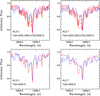 |
Fig. 6 AL 3-3 and AL 3-7: hydrogen Brackett 16 line computed for Teff = 4250, 4500, 4750, 5000 K (upper panels) and adopted values of 4250 and 4750 K, respectively (lower panels). The dashed line is the observed spectrum. |
Adopted stellar parameters for individual stars in NGC 6558, AL 3, and HP 1, and resulting C, N, O abundances.
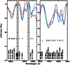 |
Fig. 7 AL 3-6: tentative fit to this low S/N spectrum, showing that it is compatible with a high CNO abundance. Blue and black lines: same observed spectrum normalized in two different ways. Red and cyan lines: synthetic spectra computed with [C/Fe] = 0.7 (red), 0.8 (cyan), [N/Fe] = +1.0, [O/Fe] = +0.8. |
6.2 AL-3and HP 1
There is a clear contrast between the spectra of HP1-5, AL3-3, and AL3-7, that have shallow lines, and AL3-6 and NGC 6558-42, that show strong lines. Whereas NGC 6558-42 is a typical red giant, the stars AL3-3, AL3-7, and HP1-5 show weak molecular lines. From the location of stars AL3-3 and AL3-7 in the CMD of Fig. 5, they should be AGB stars. In Fig. 10, we show the observed spectrum in the selected wavelength regions containing CN, OH lines, and the CO bandhead at 15 578 Å for stars AL3-3, AL3-7, and HP1-5. The molecular lines are very shallow, due to a combinationof warm temperatures and low metallicities. Clearly, the CNO abundances derived for these stars are less reliable than for the cool star NGC 6558-F42. Their CNO abundances are compatible with being close to solar, but given the shallowness of the lines, it is clear that the molecular lines are not reliable for abundance measurements.
AL3-6 instead shows very strong CNO lines. Figure 7 indicates that [C/Fe] = +0.7, 0.8, [N/Fe] = +1.0, [O/Fe] = +0.8 for this star. We show two different renormalisations to illustrate the difficulty in analysing this spectrum. Additionally, the computations with two different carbon abundances illustrate the extreme sensitivity of the lines. Clearly, however, there is an urgent need to observe this star in the optical and/or in a more extended wavelength region in the H-band to obtain firm conclusions on the CNO abundances of AL 3.
6.3 Errors
The main uncertainty in the derivation of CNO abundances in AL 3 stems from the effective temperatures. Adopting a colour excess E(B–V) = 0.36 the photometric magnitudes results in temperatures of ~5000 K. In order to be compatible with the wings of hydrogen lines, we would have to adopt E(B–V) = 0.2, but the present fit of the CMD confirms the high reddening value.
Hydrogen line wings that we adopted are a very good temperature indicator, and the temperatures can be roughly derived for the two stars showing the line, whereas for the cooler star AL3-6, the H line is not strong, indicating that it is cooler than the other two stars. For this star, we adopted Teff = 4150 K, compatible with its almost absent hydrogen-profile and a temperature compatible with its location in the RGB. With this temperature, we obtained high CNO values and could not converge with lower values. We note that the CN, CO, and OH dissociation equilibrium interplay gives a strong constraint on the result, but at the same time, these are very sensitive to abundance variations. We adopted effective temperature errors of ± 250 K for AL3-6, and ± 150 K for AL3-3 and AL3-7, errors of ±0.8 for the gravity, and ±0.3 for metallicity.
6.4 Orbits of AL 3
In order to investigate whether AL 3 belongs to the bulge, thick disc, or halo, given its solar CNO abundances, we carried out the calculations of orbits for the cluster. We have found two discrepant values of radial velocity for the 3 stars studied. For AL3-3 and AL3-7 we find a mean heliocentric radial velocity of vr = −57.93 km s−1, whereas for AL3-6 we find vr = −29.57 km s−1, compatible the value of vr = −29.38 km s−1 given in Baumgardt et al. (2019). Given that in Pérez-Villegas et al. (2020) we had computed the orbits of AL3 adopting vr = −29.38 km s−1 adopted from Baumgardt et al. (2019), we here compute the orbits for the other option found from two stars, i.e., vr = −57.93 km s−1. We employed a Galactic model that includes an exponential disc made by the superposition of three Miyamoto-Nagai potentials (Smith et al. 2015), a dark matter halo with a Navarro-Frenk-White (NFW) density profile (Navarro et al. 1997), and a triaxial Ferrers bar. The total mass of the bar is 1.2 × 10¹⁰ M⊙, an angle of 25° with the Sun-major axis of the bar, and a major axis extension of 3.5 kpc. We assumed three pattern speeds of the bar Ωb = 40, 45, and 50 km s−1 kpc−1. We kept the same bar extension, even though we changed the bar pattern speed. Our Galactic model has a circular velocity V0 = 241 km s−1 at R0 = 8.2 kpc (Bland-Hawthorn & Gerhard 2016; which is also compatible with the GRAVITY Collaboration 2019), and we assumed a peculiar motion of the Sun with respect to the local circular orbit of  km s−1 (Schönrich et al. 2010).
To take into account the effects of the observational uncertainties associated with the cluster’s parameters, we generated a set of 1000 initial conditions using a Monte Carlo method considering the errors of distance, heliocentric radial velocity, and absolute proper motion components. With such initial conditions, we integrated the orbits forward for 10 Gyr using the NIGO tool (Rossi 2015).
In Fig. 11, we show the probability density map of the orbits of AL 3 in the x − y and R − z projections co-rotating with the bar, using the two adopted distances, 6.0 kpc (Ortolani et al. 2006) and present work and 6.5 kpc (Baumgardt et al. 2019). The yellow colour displays the space region that the orbits of AL 3 cross more frequently. The black curves are the orbits using the central values of the observational parameters. In Fig. 12, we show histograms relating to the number of probable orbits as a function of pericentric distance (rmin), apocentric distance (rmax), maximum height above the plane (|Z|max), and eccentricity (e). In Table 5, we give the median values of the orbital parameters, and the errors provided in each column are derived considering the 16th and 84th percentiles of the distribution. The orbital parameters are similar for the three pattern speeds. From the apocentric distance, we can see that AL 3 is mostly confined within ~ 4 kpc, and it has a high probability to belong to the bulge component (~88%) when the adopted distance is 6.5 kpc. However, a significant fraction of orbits can reach apocentric distances up to ~ 6 kpc, indicating that AL 3 could belong to the disc component, with a non-negligible probability (~ 12%).
In Fig. 12, we show histograms relating to the number of probable orbits as a function of pericentric distance (rmin), apocentric distance (rmax), maximum height abovethe plane (|Z|max), and eccentricity. If a distance of 6.5 kpc is adopted, then it is clear that AL 3 is a very central cluster, with a maximum height reaching at most Z ~ 1.5 kpc, and with a high eccentricity orbit. This is typical of the very old, moderately metal-poor globular clusters of the Galactic bulge, similar to NGC 6522, NGC 6558, and HP 1.
On the other hand, if a distance of 6.0 kpc is adopted, according to Ortolani et al. (2006), the cluster reaches distances farther from the Galactic centre with lower eccentricities (see left and bottom and top panels of Figs. 11 and 12, respectively). The probabilities also change to an ~60% probability of belonging tothe bulge and ~40% to the disc. With this distance, the probability of being part of the disc increases significantly, and maybe this result could be more consistent with the solar CNO abundances.
Finally, a comparison of the orbital analysis of AL3 presented in Pérez-Villegas et al. (2020), where we adopted the heliocentric radial velocity of ~ −30 km s−1 (Baumgardt et al. 2019), with the one performed in the present work, assuming the heliocentric radial velocity of ~ −58 km s−1 and the same distance of 6.5 kpc, the probability to belong to the bulge component decreased from ~94% to ~88% and the probability to belong to the disk component increased from ~6% to ~12%.
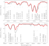 |
Fig. 8 NGC 6558-42: line identification in the range 15 527–15 555 Å. Dashed line: observed spectrum. Solid red line: synthetic spectrum. Synthetic spectrum computed with [C/Fe] = −0.5, [N/Fe] = 0.8, [O/Fe] = +0.5. |
Median orbital parameters and membership probability of AL 3.
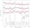 |
Fig. 10 HP 1-5, AL 3-3, and AL 3-7: spectrum in selected wavelength regions containing CN, OH lines and the CO bandhead. Synthetic spectra are computed for the CNO abundances given in Table 4. |
7 Conclusions
We analysed spectra of individual stars of the globular clusters AL 3, NGC 6558, and HP 1, obtained with the PHOENIX spectrograph at the Gemini South telescope. With a high spectral resolution of R ~ 75 000, in the H band centred at 15 555 Å, the wavelength coverage is short (15 520–15 590 Å).
In AL 3, this limited wavelength range means that it is difficult to use atomic lines to deduce the stellar parameters effective temperature, gravity, and metallicity. For this reason, we obtained the effective temperature from the Hydrogen Brackett 16 line, gravity from photometric data, and isochrones. The metallicity [Fe/H] ~ −1.3 ± 0.3 was deducedfrom the observed CMD given in Ortolani et al. (2006) and is confirmed in the present work through analysis of the same CMD. We note that we adopted [Fe/H] = −1.0 for the analysed stars, due to spectroscopic evidence. For NGC 6558 and HP 1, the stellar parameters were adopted from previous analyses from optical spectra (Barbuy et al. 2007, 2018c), and Barbuy et al. (2006, 2016) respectively. Adopting these stellar parameters, we computed the synthetic spectra in order to derive the abundances of C, N, and O. Since they vary interdependently, the fit was done iteratively, where particular attention was given to the CO bandhead. The stars analysed in NGC 6558 and HP 1 show typical CNO abundances of red giants, and confirm previous oxygen abundance derivation.
AL 3 is a more complex case: two stars analysed in AL 3 show solar CNO abundance ratios, but based on very shallow lines, and the location of these two stars in the CMD point to them being AGB stars. The star AL3-6 shows instead very strong CNO abundances of the order of [C/Fe] = +0.8, [N/Fe] = +1.0, [O/Fe] = +0.8. A strong CNO abundance indicated by this cooler star shows that AL 3 appears to be an extremely interesting old cluster. In conclusion, further investigations of this cluster are clearly needed. We also derived the cluster’s radial velocity, which in turn allowed us to compute the cluster orbits. For the two AGB stars, we found a higher velocity, whereas for the third cooler star, the radial velocity is compatible with the value from Baumgardt et al. (2019).
The orbital behaviour of AL 3 indicates that it is a typical inner bulge, moderately metal-poor globular cluster if its distance to the Sun is 6.5 kpc (Baumgardt et al. 2019), but if the distance is 6.0 kpc (Ortolani et al. 2006 and present work), there is an increased probability of AL 3 belonging to a disc component. We derive a very old age for AL 3 of 13.4 Gyr, adding AL 3 to the list of relic moderately metal-poor old clusters together with NGC 6522, NGC 6558, and HP 1 among others. Therefore, we conclude that the cluster AL 3 appears to be an extremely interesting cluster that should be further investigated through more wavelength-extended spectra, and including larger samples of member stars.
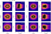 |
Fig. 11 Probability density map for x − y and R − z projections of the set of orbits for AL 3 for distances of 6.0 kpc (left panels) and 6.5 kpc (right panels), using three different values of Ωb = 40, 45, and 50 km s−1 kpc−1. The orbits are co-rotating with the bar frame. Yellow corresponds to the larger probabilities. The black lines show the orbits using the central values. |
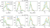 |
Fig. 12 Distribution of orbital parameters for AL 3, for distances of 6.0 kpc (top panels) and 6.5 kpc (bottom panels), with pericentric distance rmin, apocentric distance rmax, maximum vertical excursion from the Galactic plane |z|max, and eccentricity e. The colours show the different pattern speed of the bar, Ωb = 40 (blue), 45 (orange), and 50 (green) km s−1 kpc−1. |
Acknowledgements
B.B., H.E., R.R., J.M., and E.B. acknowledge grants from FAPESP, CNPq and CAPES – Financial code 001. T.M. acknowledges FAPESP postdoctoral fellowship no. 2018/03480-7. A.P.V. acknowledges FAPESP postdoctoral fellowship no. 2017/15893-1. Support for M.Z. is provided by Fondecyt Regular 1191505, the BASAL CATA Center for Astrophysics and Associated Technologies through grant PFB-06, and ANID – Millennium Science Initiative Project ICN12_009, awarded to the Millenium Institute of Astrophysics (MAS). S.O. acknowledges the partial support of the research program DOR1901029, 2019, and the project BIRD191235, 2019 of the University of Padova.
Appendix A Isochrone fitting – corner plot
The SIRIUS code performs the isochrone fitting through the construction of the Markov chain Monte Carlo (MCMC) algorithms. The purpose of the MCMC method is to obtain the posterior distribution of each parameter via the generation of random samples. Figure A.1 shows the corner plots, that is, a graphical representation of the 4D parameter space of the isochrone fitting (age, reddening, distance, and metallicity). The histograms represent the cumulative best solutions (posterior distribution) for each parameter, while the 2D density maps show the correlations between the parameters as well as the region with the highest density. To represent the posterior distributions of each parameter, we adopt the region of highest density as the central value and the uncertainties calculated from the 16th and 84th percentiles.
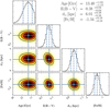 |
Fig. A.1 Corner plots representing the 4D parameter space of the Markov chain constructed through the Monte Carlo algorithm for the isochrone fitting. To represent the solutions, we adopt the peak of the distribution as the best value, and the uncertainties are computed using the 16th and 84th percentiles. More details are available in Souza et al. (2020). |
References
- Alonso, A., Arribas, S., & Martínez-Roger, C. 1998, A&AS, 131, 209 [NASA ADS] [CrossRef] [EDP Sciences] [Google Scholar]
- Alonso, A., Arribas, S., & Martínez-Roger, C. 1999, A&AS, 140, 261 [NASA ADS] [CrossRef] [EDP Sciences] [Google Scholar]
- Andrews, A.D., & Lindsay, E. M. 1967, IrAJ, 8, 126 [Google Scholar]
- Barbuy, B., Zoccali, M., Ortolani, S., et al. 2006, A&A, 449, 349 [NASA ADS] [CrossRef] [EDP Sciences] [Google Scholar]
- Barbuy, B., Zoccali, M., Ortolani, S., et al. 2007, AJ, 134, 1613 [NASA ADS] [CrossRef] [Google Scholar]
- Barbuy, B., Cantelli, E., Vemado, A. et al. 2016, A&A, 591, A53 [NASA ADS] [CrossRef] [EDP Sciences] [Google Scholar]
- Barbuy, B., Chiappini, C., & Gerhard, O. 2018a, ARA&A, 56, 223 [Google Scholar]
- Barbuy, B., Trevisan, J., & de Almeida, A. 2018b, PASA, 35, 46 [NASA ADS] [CrossRef] [Google Scholar]
- Barbuy, B., Muniz, L., Ortolani, S. et al. 2018c, A&A, 619, A178 [NASA ADS] [CrossRef] [EDP Sciences] [Google Scholar]
- Baumgardt, H., Hilker, M., Sollima, A., & Bellini, A. 2019, MNRAS, 482, 5138 [Google Scholar]
- Bessell, M. S. 1979, PASP, 91, 589 [NASA ADS] [CrossRef] [Google Scholar]
- Bica, E., Ortolani, S., & Barbuy, B. 2016, PASA, 33, 28 [Google Scholar]
- Blanco, V. M. 1988, AJ, 95, 1400 [NASA ADS] [CrossRef] [Google Scholar]
- Bland-Hawthorn, J., & Gerhard, O. 2016, ARA&A, 54, 529 [NASA ADS] [CrossRef] [EDP Sciences] [Google Scholar]
- Bressan, A., Marigo, P., & Girardi, L. 2012, MNRAS, 427, 127 [NASA ADS] [CrossRef] [Google Scholar]
- Carpenter, J. M. 2001, AJ, 121, 2851 [NASA ADS] [CrossRef] [Google Scholar]
- Dias, B., Barbuy, B., Saviane, I. et al. 2015, A&A, 573, A13 [NASA ADS] [CrossRef] [EDP Sciences] [Google Scholar]
- Dias, B., Barbuy, B., Saviane, I. et al. 2016, A&A, 590, A9 [NASA ADS] [CrossRef] [EDP Sciences] [Google Scholar]
- Dotter, A., Chaboyer, B., Jevremović, D. et al. 2008, ApJS, 178, 89 [Google Scholar]
- Dufay, J., Berthier, P., & Morignat, B. 1954, Publ. of the OHP, 3, No. 17 [Google Scholar]
- Gaia Collaboration (Brown, A. G. A., et al.) 2021, A&A, in press, https://doi.org/10.1051/0004-6361/202039657 [Google Scholar]
- GRAVITY Collaboration (Abuter, R., et al.) 2019, A&A, 625, L10 [NASA ADS] [CrossRef] [EDP Sciences] [Google Scholar]
- Goldman, A., Schoenfeld, W.G., Goorvitch, D. et al. 1998, J. Quant. Spectr. Rad. Transf., 59, 453 [Google Scholar]
- Goorvitch, D. 1994, ApJS, 95, 535 [NASA ADS] [CrossRef] [Google Scholar]
- Gustafsson, B., Edvardsson, B., Eriksson, K., et al. 2008, A&A, 486, 951 [NASA ADS] [CrossRef] [EDP Sciences] [Google Scholar]
- Harris, W. E. 1996, AJ, 112, 1487 [NASA ADS] [CrossRef] [Google Scholar]
- Hinkle, K., Wallace, L., & Livingston, W. 1995, PASP, 107, 1042 [NASA ADS] [CrossRef] [Google Scholar]
- Huber, K. P., & Herzberg, G. 1979, Constants of Diatomic Molecules (Boston, MA: Springer) [Google Scholar]
- Jorgensen, U. G. 1994, A&A, 284, 179 [NASA ADS] [Google Scholar]
- Kerber, L. O., Libralato, M., Souza, S. O., et al. 2019, MNRAS, 484, 5530 [NASA ADS] [CrossRef] [Google Scholar]
- Lauberts, A. 1982, ESO/Uppsala Survey of ESO(B) Atlas, ESO, Garching [Google Scholar]
- Lecureur, A., Hill, V., Zoccali, M., et al. 2007, A&A, 465, 799 [NASA ADS] [CrossRef] [EDP Sciences] [Google Scholar]
- Majewski, S. R., Schiavon, R. P., & Frinchaboy, P. M. 2017, AJ, 154, 94 [NASA ADS] [CrossRef] [Google Scholar]
- Meléndez, J., & Barbuy, B. 1999, ApJS, 124, 527 [NASA ADS] [CrossRef] [MathSciNet] [Google Scholar]
- Meléndez, J., & Barbuy, B. 2002, ApJ, 575, 474 [Google Scholar]
- Meléndez, J., Barbuy, B., & Spite, F. 2001, ApJ, 556, 858 [NASA ADS] [CrossRef] [Google Scholar]
- Meléndez, J., Barbuy, B., Bica, E. et al. 2003, A&A, 411, 417 [NASA ADS] [CrossRef] [EDP Sciences] [Google Scholar]
- Navarro, J. F., Frenk, C. S., & White, S. D. M. 1997, ApJ, 490, 493 [NASA ADS] [CrossRef] [Google Scholar]
- Ortolani, S., Bica, E., & Barbuy, B. 1997, MNRAS, 284, 692 [NASA ADS] [Google Scholar]
- Ortolani, S., Bica, E., & Barbuy, B. 2006, ApJ, 646, L115 [NASA ADS] [CrossRef] [Google Scholar]
- Pérez-Villegas, A., Rossi, L., Ortolani, S., et al. 2018, PASA, 35, 21 [Google Scholar]
- Pérez-Villegas, A., Barbuy, B., Kerber, L. et al. 2020, MNRAS, 491, 3251 [Google Scholar]
- Pietrinferni, A., Cassisi, S., Salaris, M., & Castelli, F. 2006, ApJ, 642, 797 [NASA ADS] [CrossRef] [Google Scholar]
- Piskunov, N., Kupka, F., Ryabchikova, T., Weiss, W., & Jeffery, C. 1995, A&AS, 112, 525 [NASA ADS] [Google Scholar]
- Rich, R. M., Ortolani, S., Bica, E., & Barbuy, B. 1998, AJ, 116, 1295 [NASA ADS] [CrossRef] [Google Scholar]
- Rossi, L. J. 2015, Astron. Comput., 12, 11 [NASA ADS] [CrossRef] [Google Scholar]
- Rossi, L., Ortolani, S., Bica, E., Barbuy, B., & Bonfanti, A. 2015, MNRAS, 450, 3270 [NASA ADS] [CrossRef] [Google Scholar]
- Ryabchikova, T., Piskunov, N., Kurucz, R. L. et al. 2015, Phy. Scr., 90, 054005 [Google Scholar]
- Schiavon, R. P., & Barbuy, B. 1999, ApJ, 510, 934 [NASA ADS] [CrossRef] [Google Scholar]
- Schönrich, R., Binney, J., & Dehnen, W. 2010, MNRAS, 403, 1829 [NASA ADS] [CrossRef] [Google Scholar]
- Souza, S. O., Kerber, L. O., Barbuy, B. et al. 2020, ApJ, 890, 38 [CrossRef] [Google Scholar]
- Shetrone, M., Bizyaev, D., Lawler, J. E. et al. 2015, ApJS, 221, 24 [Google Scholar]
- Skrutskie, M. F., Cutri, R. M., Stiening, R. et al. 2006, AJ, 131, 1163 [NASA ADS] [CrossRef] [Google Scholar]
- Smith, R., Flynn, C., Candlish, G. N., Fellhauer, M., & Gibson, B. K. 2015, MNRAS, 448, 2934 [NASA ADS] [CrossRef] [Google Scholar]
- Soto, M., Barbá, R., Gunthardt, G., et al. 2013, A&A, 552, A101 [NASA ADS] [CrossRef] [EDP Sciences] [Google Scholar]
- van den Bergh, S., & Hagen, G. L. 1975, AJ, 80, 11 [NASA ADS] [CrossRef] [Google Scholar]
- VVV Collaboration (Saito, R., et al.) 2012, A&A, 537, A107 [NASA ADS] [CrossRef] [EDP Sciences] [Google Scholar]
All Tables
Adopted stellar parameters for individual stars in NGC 6558, AL 3, and HP 1, and resulting C, N, O abundances.
All Figures
|
Fig. 1 AL 3: 3 min B image with the three sample stars identified. Extraction of 3′ × 3′. North is up and east is left. |
| In the text | |
|
Fig. 2 AL 3-3: radial velocity derivation. The solid black line is the observed spectrum, the solid grey line is the noise spectrum, the solid red line is the synthetic spectrum, the dashed red lines are those used to derive the radial velocity, and the dashed black lines are the OH sky lines. |
| In the text | |
|
Fig. 3 AL 3-7: radial velocity derivation. The solid black line is the observed spectrum, the solid grey line is the noise spectrum, the solid red line is the synthetic spectrum, the dashed red lines are those used to derive the radial velocity, and the dashed black lines are the OH sky lines. |
| In the text | |
|
Fig. 4 AL 3-6: radial velocity derivation. The solid black line is the observed spectrum, the solid grey line is the spectrum of star AL3-7, the dashed red lines are those used to derive the radial velocity, and the dashed black lines are the OH sky lines. |
| In the text | |
|
Fig. 5 AL 3 V vs. V − I CMD. The black dots are the stars within 120 pixels from the cluster centre (see Ortolani et al. 2006). The red stars are the observed stars of the present work. The solid blue line represents the median solution of the isochrone fitting, while the blue region reveals the solutions within 1 − σ from Dartmouth isochrones, and the rose region corresponds to BaSTI solutions for the AGB. |
| In the text | |
|
Fig. 6 AL 3-3 and AL 3-7: hydrogen Brackett 16 line computed for Teff = 4250, 4500, 4750, 5000 K (upper panels) and adopted values of 4250 and 4750 K, respectively (lower panels). The dashed line is the observed spectrum. |
| In the text | |
|
Fig. 7 AL 3-6: tentative fit to this low S/N spectrum, showing that it is compatible with a high CNO abundance. Blue and black lines: same observed spectrum normalized in two different ways. Red and cyan lines: synthetic spectra computed with [C/Fe] = 0.7 (red), 0.8 (cyan), [N/Fe] = +1.0, [O/Fe] = +0.8. |
| In the text | |
|
Fig. 8 NGC 6558-42: line identification in the range 15 527–15 555 Å. Dashed line: observed spectrum. Solid red line: synthetic spectrum. Synthetic spectrum computed with [C/Fe] = −0.5, [N/Fe] = 0.8, [O/Fe] = +0.5. |
| In the text | |
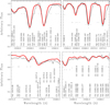 |
Fig. 9 NGC 6558-42: same as Fig. 8, in the range 15 555–15 587 Å. |
| In the text | |
|
Fig. 10 HP 1-5, AL 3-3, and AL 3-7: spectrum in selected wavelength regions containing CN, OH lines and the CO bandhead. Synthetic spectra are computed for the CNO abundances given in Table 4. |
| In the text | |
|
Fig. 11 Probability density map for x − y and R − z projections of the set of orbits for AL 3 for distances of 6.0 kpc (left panels) and 6.5 kpc (right panels), using three different values of Ωb = 40, 45, and 50 km s−1 kpc−1. The orbits are co-rotating with the bar frame. Yellow corresponds to the larger probabilities. The black lines show the orbits using the central values. |
| In the text | |
|
Fig. 12 Distribution of orbital parameters for AL 3, for distances of 6.0 kpc (top panels) and 6.5 kpc (bottom panels), with pericentric distance rmin, apocentric distance rmax, maximum vertical excursion from the Galactic plane |z|max, and eccentricity e. The colours show the different pattern speed of the bar, Ωb = 40 (blue), 45 (orange), and 50 (green) km s−1 kpc−1. |
| In the text | |
|
Fig. A.1 Corner plots representing the 4D parameter space of the Markov chain constructed through the Monte Carlo algorithm for the isochrone fitting. To represent the solutions, we adopt the peak of the distribution as the best value, and the uncertainties are computed using the 16th and 84th percentiles. More details are available in Souza et al. (2020). |
| In the text | |
Current usage metrics show cumulative count of Article Views (full-text article views including HTML views, PDF and ePub downloads, according to the available data) and Abstracts Views on Vision4Press platform.
Data correspond to usage on the plateform after 2015. The current usage metrics is available 48-96 hours after online publication and is updated daily on week days.
Initial download of the metrics may take a while.