| Issue |
A&A
Volume 648, April 2021
|
|
|---|---|---|
| Article Number | A122 | |
| Number of page(s) | 14 | |
| Section | Numerical methods and codes | |
| DOI | https://doi.org/10.1051/0004-6361/202038981 | |
| Published online | 26 April 2021 | |
Machine learning technique for morphological classification of galaxies from the SDSS
I. Photometry-based approach⋆
1
Main Astronomical Observatory of the National Academy of Sciences of Ukraine, 27 Akademik Zabolotny St., Kyiv 03143, Ukraine
e-mail: This email address is being protected from spambots. You need JavaScript enabled to view it.
2
Institute of Physics of the National Academy of Sciences of Ukraine, 46 avenue Nauka, Kyiv 03028, Ukraine
3
Institute of Astronomy, V.N. Karazin Kharkiv National University, 35 Sumska St., Kharkiv 61022, Ukraine
Received:
20
July
2020
Accepted:
1
February
2021
Abstract
Context. Machine learning methods are effective tools in astronomical tasks for classifying objects by their individual features. One of the promising utilities is related to the morphological classification of galaxies at different redshifts.
Aims. We use the photometry-based approach for the SDSS data (1) to exploit five supervised machine learning techniques and define the most effective among them for the automated galaxy morphological classification; (2) to test the influence of photometry data on morphology classification; (3) to discuss problem points of supervised machine learning and labeling bias; and (4) to apply the best fitting machine learning methods for revealing the unknown morphological types of galaxies from the SDSS DR9 at z < 0.1.
Methods. We used different galaxy classification techniques: human labeling, multi-photometry diagrams, naive Bayes, logistic regression, support-vector machine, random forest, k-nearest neighbors.
Results. We present the results of a binary automated morphological classification of galaxies conducted by human labeling, multi-photometry, and five supervised machine learning methods. We applied it to the sample of galaxies from the SDSS DR9 with redshifts of 0.02 < z < 0.1 and absolute stellar magnitudes of −24m < Mr < −19.4m. For the analysis we used absolute magnitudes Mu, Mg, Mr, Mi, Mz; color indices Mu − Mr, Mg − Mi, Mu − Mg, Mr − Mz; and the inverse concentration index to the center R50/R90. We determined the ability of each method to predict the morphological type, and verified various dependencies of the method’s accuracy on redshifts, human labeling, morphological shape, and overlap of different morphological types for galaxies with the same color indices. We find that the morphology based on the supervised machine learning methods trained over photometric parameters demonstrates significantly less bias than the morphology based on citizen-science classifiers.
Conclusions. The support-vector machine and random forest methods with Scikit-learn software machine learning library in Python provide the highest accuracy for the binary galaxy morphological classification. Specifically, the success rate is 96.4% for support-vector machine (96.1% early E and 96.9% late L types) and 95.5% for random forest (96.7% early E and 92.8% late L types). Applying the support-vector machine for the sample of 316 031 galaxies from the SDSS DR9 at z < 0.1 with unknown morphological types, we found 139 659 E and 176 372 L types among them.
Key words: galaxies: general / methods: data analysis / galaxies: statistics / galaxies: photometry / galaxies: spiral / galaxies: elliptical and lenticular, cD
The catalog is only available at the CDS via anonymous ftp to cdsarc.u-strasbg.fr (130.79.128.5) or via http://cdsarc.u-strasbg.fr/viz-bin/cat/J/A+A/648/A122
© ESO 2021
1. Introduction
During the 1990s, artificial neural network (ANN) algorithms were implemented for the automatic morphological classification of galaxies since the huge extragalactic data sets had been conducted. The classification accuracy (success rate) of the ANNs was from 65% to 90% depending on the mathematical subtleties of the applied methods and the quality of the galaxy samples. One of the first of these works was done by Storrie-Lombardi et al. (1992) with a feed-forward neural network, which dealt with the classification of 5217 galaxies into five classes (E, SO, Sa-Sb, Sc-Sd, and Irr) with a 64% accuracy. A detailed comparison of human and neural classifiers was presented by Naim et al. (1995), who used a principal component analysis to classify 831 galaxies; the best result was with an rms deviation of 1.8 T-types. Summarizing the first attempts, Lahav et al. (1995, 1996) resulted that “the ANNs can replicate the classification by a human expert almost to the same degree of agreement as that between two human experts, to within 2 T-type units”.
An excellent introduction to the classification algorithms for astronomical tasks, including the morphological galaxy classification, is given in various studies (Ball & Brunner 2010; Way et al. 2012; VanderPlas et al. 2012; Ivezic et al. 2014; Al-Jarrah et al. 2015; Fluke & Jacobs 2020; El Bouchefry & de Souza 2020; Vavilova et al. 2020a). We also refer to the classical work by Buta (2011), and to a good pedagogical review by Conselice et al. (2014) with a discussion of principal methods in which galaxies are studied morphologically and structurally.
The Sloan Digital Sky Survey (SDSS), which started in 2000, collected more data in its first few weeks than had been amassed in the history of astronomy. Now, 20 years later, its archive contains about 170 terabytes of information. Soon its successor, the Large Synoptic Survey Telescope (LSST), will acquire that quantity of data every five days (York et al. 2000). It provided entry points for the computer scientists who want to engage in astronomical research, and explains why big data mining and machine learning methods are gaining such popularity: they are able to categorize celestial bodies in big data sets with more accuracy than ever.
In this context we review below several works where different approaches were developed and great efforts were made to identify the morphological types of galaxies from the SDSS in the visual and in the automated modes.
Ball et al. (2004) tested a supervised ANN for 50 morphological classifications and found that it can be used without human intervention for the SDSS galaxies (correlations between predicted and actual properties were around 0.9 with rms errors on the order of 10%). de la Calleja & Fuentes (2004) developed a method that combines two machine learning algorithms: locally weighted regression and ANN. They tested it with 310 images of galaxies from the New General Catalogue and obtained an accuracy of 95.11% and 90.36%, respectively. Kasivajhula et al. (2007) explored support-vector machine, random forest, and naive Bayes algorithms as the galaxy image classifiers, and principal component analysis for the direct image pixel data compressing, but favored random forest. They cited the opinion of several astronomers on the successful perspective of galaxy classification by morphological features as “one of the most cumbersome areas in celestial classification, and the one that has proven the most difficult to automate”. Nevertheless, Andrae et al. (2010) applied a probabilistic classification algorithm to classify the SDSS bright galaxies and obtained that it produces reasonable morphological classes and object-to-class assignments without any prior assumptions.
For the visual morphological classification conducted during recent years, we note the following: Nair & Abraham (2010) prepared the detailed visual classifications for 14 034 galaxies from the SDSS DR4 at z < 0.1, which can be used as a good training sample to calibrate the automated galaxy classification algorithms. Banerji et al. (2010) provided a significant study where galaxies from the Galaxy Zoo Project1 formed a training sample for morphological classifications of galaxies from the SDSS DR6 into three classes (early types, spirals, spam objects). These authors showed, at a high confidence level, that using a set of certain galaxy parameters, a neural network can reproduce human classifications to better than 90% for all these classes, and the Galaxy Zoo catalog (GZoo1) can serve as a training sample.
Hundreds of thousands of volunteers were involved in the Galaxy Zoo project (GZoo) to make a visual classification of a million galaxies in the SDSS (Lintott et al. 2008). Most of their results have found good scientific applications. For example, using the raw imaging data from SDSS that was available in the GZoo1, and the handpicked features of galaxies from the SDSS, Kates-Harbeck (2012) applied a logistic regression classifier and attained 95.21% classification accuracy. Willett et al. (2013) issued a new catalog of morphological types from the GZoo2 Project in synergy with the SDSS DR7, which contains more than 16 million morphological classifications of 304 122 galaxies and their finer morphological features (bulges, bars, and the shapes of edge-on disks as well as parameters of the relative strengths of galactic bulges and spiral arms). Simmons et al. (2017) cross-verified 48 000 galaxies from the CANDELS survey and their detailed morphological features from the GZoo (clumpiness, bar instabilities, spiral structure, merging). It allowed them to create a list of galaxies with featureless disks at 1 ≤ z ≤ 3, which may represent “a dynamically warmer progenitor population to the settled disk galaxies seen at later epochs”.
Kuminski & Shamir (2016) have generated a morphology catalog of the SDSS galaxies with the Wndchrm image analysis utility using the nearest neighbor classifier. They pointed out that about 900 000 of the instances classified as spirals and about 600 000 of those classified as ellipticals have a statistical agreement rate of about 98% with the GZoo classification. Murrugarra & Hirata (2017) evaluated a convolutional neural network to classify galaxies from the SDSS into two classes (ellipticals and spirals) by image processing, and attained an accuracy of 90–91%. Using the same machine learning technique, the convolutional neural network and especially the inception method, Rahman & Azhari (2018) conducted classification into three general categories: ellipticals, spirals, and irregulars. They used 710 images (206 E, 320 Sp, 184 Irr) and obtained that images after processing showed a relatively low testing accuracy compared to those that did not undergo any form of image processing. Their best testing accuracy was 78.3%.
Supervised and unsupervised methods were both applied by Gauthier et al. (2016) to study the GZoo data set of 61 578 pre-classified galaxies (spiral, elliptical, round, disk). They found that the variation in galaxy images is correlated with brightness and eccentricity, and that the random forest method gives the best accuracy (67%); meanwhile, its combination with regression to predict the probabilities of galaxies associated with each class can reach 94% accuracy. Beck et al. (2018) analyzed the integration of visual labeling and automated morphological assignment with random forest for more than 200 000 galaxies from the GZoo2 project. They managed to show that such a combination increases the binary classification rate with quite good accuracy (93.1%), focusing on the velocity, one of the four Vs of astronomical data (volume, variety, velocity, and value).
The photometric and spectral parameters of each object, as well as their images, are available through the SDSS website. It uses a well-known fact that galaxy morphological type is correlated with several parameters, for example the color indices, luminosity, de Vaucouleurs radius, and inverse concentration index. In our series of works we have demonstrated the effectiveness of a combination of the visual classification and the two-dimensional diagrams of color indices g − i and one of the parameters mentioned above (Vavilova et al. 2009, 2015; Melnyk et al. 2012; Dobrycheva & Melnyk 2012). Specifically, using the color indices versus inverse concentration index diagrams for each galaxy with radial velocities 3000 < V < 9500 km s−1 from the SDSS DR5, we obtained criteria for separating the galaxies into three classes, namely (E) early types–elliptical and lenticular, (S) spiral Sa − Scd, and (LS) late spiral Sd − Sdm and irregular Im/BCG galaxies (Melnyk et al. 2012).
Making a ternary automated morphological galaxy classification we attained good accuracy: 98% for E, 88% for S, and 57% for LS. We applied this approach based on the photometric data alone (multi-parametric diagrams) to classify a sample of 316 031 SDSS galaxies at 0.003 ≤ z ≤ 0.1 from the SDSS DR9 (142 979 E, 112 240 S, 60 812 L; Dobrycheva 20132). The criterion was determined visually by the graph of the relationship between these two values. In each graph we indicated the regions where there are a maximum number of galaxies of morphological types E, S, and LS and a minimum number of other morphological types. At that time, we used the training sample as a test sample, which means that the actual accuracy was at least a few percentage points lower. A more detailed explanation is given by Dobrycheva et al. (2018).
The ternary classification is a partial case of decision tree classifier and provides an accuracy level of morphological classification that is not very high. We tried to use other more sophisticated machine learning methods and to compare them. In works by Dobrycheva (2017), the results on a binary morphological classification of this sample using software with an open-source KNIME Analytics Platform ver. 3.5.0 were presented, and three machine learning methods were compared: naive Bayes, random forest, and support-vector machine based on WEKA 3.7 software and neural networks (RProp MLP). It turned out that the random forest method provided the highest accuracy: 91% of galaxies were correctly classified (96% for E type and 80% for L type).
The higher rate of morphological classification was accessed with convolutional neural network (CNN) when the imaging data was analyzed. We note some recent works where galaxy samples in the Local Universe were studied.
Sreejith et al. (2018) exploited 7528 galaxies from the Galaxy and Mass Assembly (GAMA) survey with 0.002 < z < 0.06. These galaxies were previously visually classified independently by three classifier teams. The statistical machine learning algorithms were trained on a set of 6022 objects (80% of the data set) using ten independent distance parameters. These algorithms were subsequently tested on the remaining 20% of the data set to classify them into five galaxy types: elliptical, little blue spheroid, early-type spirals (S0-SBa), intermediate-type spirals (Sab-SBcd), and late-type spirals–irregulars (Sd-Irr). Their results were as follows: support-vector machine – 75.8%, neural networks – 76.0%, classification trees – 69.0%, and classification trees with random forest – 76.2%. Cheng et al. (2020) used the Dark Energy Survey data combined with human labeling from the GZoo1 project to compare the effectiveness of several machine learning methods, among which CNN, k-nearest neighbors, logistic regression, support-vector machine, random forest, and neural networks. These authors obtained that CNN is the most successful method for the binary morphological classification dealing with galaxy images; using a sample of ∼2800 galaxies at z < 0.25, they attained an accuracy of ∼99%.
Barchi et al. (2020) produced a catalog with morphological data for 670 560 galaxies at 0.03 < z < 0.1, where the input data were taken from SDSS-DR7 (Petrosian magnitude in r-band brighter than 17.78, and |b|> 30°). They used traditional machine learning (TML) and deep learning (DL) approaches to distinguish elliptical (E) from spiral (S) galaxies. These authors presented a non-parametric galaxy morphology system, named CyMorph, which determines concentration (C), asymmetry (A), smoothness (S), entropy (H), and gradient pattern analysis (GPA) metrics. All the studied TML methods (decision tree, support-vector machine, and multi-layer perceptron) produced a 98% overall accuracy. Despite an imbalance of types in the training set (S galaxies, 87%, and E galaxies, 13%) at least 95% accuracy and 96% recall for E systems were attained. Since S galaxies constitute most of the training set, it is not surprising that accuracy and recall were 99%, establishing a model with 99% overall accuracy for this data set. In general, the CNN method (GoogLeNet Inception) with the imbalanced data sets and 22-layer network resulted in 98.7% overall accuracy for binary morphological classification. Mittal et al. (2020) introduced the data augmentation-based MOrphological Classifier Galaxy using Convolutional Neural Networks (daMCOGCNN) and obtained a testing accuracy of 98%. Their data sets of 4614 images were collected from SDSS Image Gallery, Galaxy Zoo challenge, and Hubble Image Gallery.
It can be seen that, in general, the implemented methods with CNN provide accuracy around 98% for the morphological classification of galaxies. However, they require imaging data with a good resolution, and work well for nearby galaxies. On the contrary, in our classifiers we use easily observed photometric parameters, which could even be defined for distant galaxies.
The above brief discourse into the history of the automated morphological classification of various galaxy samples from a homogeneous Sloan Digital Sky Survey shows that classification accuracy (success rate) depends not only on the obvious factors such as the quality of the data (photometric, image, spectral) or human labeling, but also on the applied machine learning methods. Moreover, it is important to discuss not only the effectiveness of the methods, but also the problem points that are hidden in general statistics of a success rate. Specifically, they are directly related to the evolutionary features of galaxies. Here the developed tools and catalogs based on the photometric data augmentation may serve an essential role as training samples for the data analysis of upcoming biggest surveys as LSST and Euclid.
This work deals with the automated morphological classification of the low redshift galaxies from the SDSS DR9. We used the cosmological WMAP7 parameters ΩM = 0.27, ΩΛ = 0.73, Ωk = 0, H0 = 0.71 and set the following tasks:
– to verify various machine learning methods and to select most effective among them for classifying the morphological types of galaxies at z < 0.1 from the SDSS DR9;
– to determine the margins where the automated morphology classification based on the photometric parameters of galaxies gives the best result, e.g. morphological peculiarities, at different redshifts;
– to reveal typical problem points of the automated morphological classification based on the photometric data and human labeling;
– to apply the developed criteria for the automated morphological classification of galaxies at z < 0.1 from the SDSS DR9 with unknown morphological types.
We organized the paper as follows. Section 2 deals with galaxy samples. Section 3 describes the studied machine learning methods (naive Bayes, logistic regression, k-nearest neighbors, random forest, and support-vector machine) and the setting parameters used in each method. The results are presented in Sect. 4. In the discussion we raise questions about several problem points of the supervised machine learning methods for the automated galaxy morphological classification (Sect. 5.1) and compare the effectiveness of different methods (Sect. 5.2). Concluding remarks are highlighted in Sect. 6.
Our other approach dealing with the deep learning similarity to define morphological features of galaxies from this studied sample is described in the next paper by Khramtsov et al. (2020).
2. Galaxy samples from the SDSS DR9 for the automated morphological classification
2.1. Galaxy sample
A preliminary sample of galaxies at z < 0.1 with the absolute stellar magnitudes −24m < Mr < −13m from the SDSS DR9 contained ∼724 000 galaxies. Following the SDSS recommendation, we input limits mr < 17.7 by visual stellar magnitude in r-band to avoid typical statistical errors in spectroscopic flux. After excluding the images with duplicates of the same galaxy and artificial objects, the final sample contained N = 316 031 galaxies. To clear the sample from segmented images of the same galaxy, we used our code based on the minimum angle distances between such SDSS objects.
The absolute stellar magnitude of the galaxy was obtained by the formula

where mr is the visual stellar magnitude in r-band, DL the luminosity distance, extr the Galactic absorption in r-band in accordance to Schlegel et al. (1998), Kr(z) the k-correction in r-band according to Chilingarian et al. (2010), Chilingarian & Zolotukhin (2012).
The color indices were calculated as

where mg and mi are the visual stellar magnitude in g- and i-band; extg and exti the Galactic absorption in g- and i-band; and Kg(z) and Ki(z) the k-correction in g- and i-band, respectively.
A ternary morphological classification with the method of multi-parametric diagrams (in-box classification) does not attain a reasonable accuracy to classify spiral galaxies of Sa − Scd type (see Sect. 1, and Dobrycheva et al. 2015, 2018; Vavilova et al. 2020a). To verify the various supervised machine learning methods we decided to provide a binary automated morphological classification: early-type galaxies E, from ellipticals to lenticulars; late-type galaxies L, from S0a − Sdm to irregular Im/BCG galaxies.
2.2. Training samples
The supervised machine learning methods are used in the search for a relationship between the input and output data, in our case, between features of galaxies (photometric parameters) and their morphological types. A training sample should represent these features as much as possible, allowing us to generalize and to build the model for predicting the target variables (see, e.g., Kremer et al. 2017). That is why our first step before applying the machine learning methods was to compose a good quality training sample.
We visually identified the morphological types (E and L) of 6163 galaxies from the sample described in Sect. 2.1, which were randomly selected at different redshifts and with different luminosity. This is ∼2% of the total number of the studied galaxy sample. We used images from multiple bands for the visual classification.
To eliminate the human error factor, cross-validation of the same galaxies for their types and morphological features was performed by the authors of this paper. To label the galaxy types at different redshifts in the case of disputable visual classification, we took into account their spectral data for additional clarification (e.g., the presence of a strong emission line Hα for the spiral galaxy SDSS J124332.66+172004.3 at z = 0.02 and an absorption line Hβ for the elliptical galaxy SDSS J155947.57+263334.4 at z = 0.09).
Using one of the three color indices and such parameters as the inverse concentration index, absolute stellar magnitude, de Vaucouleurs radius, and scale radius (color − R50/R90, color − Mr, color − deVRadr, and color − expRadr diagrams, respectively), it is possible to carry out a reliable preliminary morphological classification without invoking visual inspection. The dependence of the color indices and the parameter R50/R90 gives the best fit because the parameter values do not depend on the radial galaxy velocity and because the selection effects are avoided (Dobrycheva & Melnyk 2012). As an example, see the diagram of inverse concentration indexes R50/R90 as a function of color indices g − i for 6163 galaxies of the training sample, which is shown in Fig. 1. It demonstrates a good separation into the early and late galaxy types (Fig. 2) and also reveals the well-known effect of color indices bimodality (Balogh et al. 2004). The overlap of morphological types in the range of Mg − Mi from 1.1 to 1.3 is still substantial and will be discussed in Sect. 5.
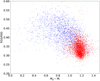 |
Fig. 1. Diagram of color indices g − i and inverse concentration indexes R50/R90 of the training sample (6163 galaxies randomly selected with different redshifts and luminosities from the SDSS DR9). The visually classified galaxies (human labeling) of early E − S0 types are shown in red, and the late Sa − Irr types in blue. |
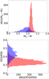 |
Fig. 2. Distribution of the morphological types (early in red, late in blue) depending on the photometric parameters: (left panel) color indices Mg − Mi, (right panel) inverse concentration index R50/R90) for the training sample of 6163 galaxies as in Fig. 1. |
3. Supervised machine learning methods and morphological classification
The learning can be supervised, semi-supervised, unsupervised, and reinforced (Burkov 2019). In our work we only used the supervised methods where the data set is a collection of the labeled examples  .
.
In our case each element xi among N is a galaxy feature vector, where each dimension j = 1, …, D contains a value that describes yi. That value is called a feature and is denoted as x(j). For instance, if each example x in our collection represents a galaxy, then the first feature, x(1), could contain absolute magnitude Mu, the second feature, x(2), could contain color indices Mu − Mr, and x(3) could contain the inverse concentration index R50/R90. Summing up, there are absolute magnitudes Mu, Mg, Mr, Mi, Mz; color indices Mu − Mr, Mg − Mi, Mr − Mz; and inverse concentration indexes R50/R90 to the center. For all examples in the data set, the feature at position j in the feature vector always contains the same kind of information. This means that if  contains color indices Mu − Mr for some example xi, then
  will also contain color indices Mu − Mr in each example xk, k = 1, …, N. The label yi can be either an element belonging to a finite set of classes 1, 2, …, T, or a real number, or a more complex structure, like a vector, a matrix, a tree, or a graph. In our work we only have two classes, E and L, where E means the early-type galaxy and L means the late morphological type.
The goal of a supervised learning algorithm is to use the data set to produce a model that takes a feature vector x as input, and outputs information that allows us to deduce the label for this feature vector. For instance, the model with a data set of galaxies could take a feature vector describing the morphological type of galaxy as the input information and a probability that the galaxy has E or L morphological type as the output information.
Using the Scikit-Learn machine learning library (ver. 0.2.2 for the Python programming language (Pedregosa et al. 2011), which is a simple tool for data mining and data analysis (see, e.g., Ivezic et al. 2014), we trained naive Bayes, random forest, support-vector machine, k-nearest neighbors, and logistic regression. To train the classifier we used the absolute magnitudes Mu, Mg, Mr, Mi, Mz; color indices Mu − Mr, Mg − Mi, Mr − Mz; and the inverse concentration index R50/R90 (Sect. 2.2).
3.1. Naive Bayes
The naive Bayes classifiers are based on the Bayes theorem and conditional independence of the features to calculate the probability of class G (in our case it is a morphological type of galaxies) with a given feature vector (set of galaxy attributes) X = (x1, …, xi):
If we accept the conditional independence assumption, instead of computing the class-conditional probability for each combination of X, we only have to estimate the conditional probability of each xi, given G. To classify a test record, the naive Bayes computes the posterior probability for each class G:
3.2. Random forest
The random forest (RF) classifiers works as follows. The training sample contains N objects whose dimension of objects feature is M (Mu, Mg, Mr, Mi, Mz, Mu − Mr, Mg − Mi, Mr − Mz, inverse concentration indexes R50/R90 to the center) and the parameter m is given (usually  ) as an incomplete number of traits for training. Then we build the committee tree; the most common way is as follows. First, we generate a random subsample with size N likely in the training sample. Thus, some objects will hit two or more times, and on average N(1 − 1/N)N, and approximately N/e objects will not hit at all. Next, we construct the decision tree that classifies the objects in this subsample. The next node of the tree in the process of creating will use not all M objects features, but only m, which are randomly chosen. Finally, we develop the tree up to the complete exhaustion of the subsample.
The classification of objects is conducted by voting: each tree of the committee puts the object into one of the classes, and the class wins if it has the most significant number of trees voted (Breiman 2001). In our case the forest consisted of 500 trees and the maximum depth of the tree was equal to 11.
3.3. Support-vector machine
We get a training data set of n points of the form (x1, y1),…,(xn, yn), where yi is either 1 or −1 (in our work it is E or L morphological type of the galaxy). Each point indicates to which type the point xi belongs (set of attributes of galaxies). Each xi is a p-dimensional real vector. We should find the “maximum-margin hyperplane” that divides the group of points xi, for which yi = 1, from the group of points, for which yi = −1 is defined in such a manner that the distance between the hyperplane and the nearest point xi from either group is maximized. Any hyperplane can be written as the set of points xi satisfying wixi − b = 0, where wi is the normal vector (not necessarily normalized) to the hyperplane. It is more likely Hesse’s normal form, except that wi is not necessarily a unit vector. The parameter  determines the offset of the hyperplane from the origin along the normal vector w (VanderPlas 2016; Cortes & Vapnik 1995).
We used the support-vector machine (SVM) with radial basis function kernel without limit on the number of iterations until the condition of the solution is fulfilled. The inverse of regularization strength index C was equal to 78 (smaller values specify stronger regularization). The parameter gamma was defined as “scale” by default.
3.4. K-nearest neighbors
The classifier based on k-nearest neighbors (k-NN) is an example of the most straightforward machine learning algorithm. It does not create class-dividing functions, but remembers the position of training sample objects in the hyperspace of features. This method’s disadvantage is that its productivity linearly depends on the size of the training sample, the dependence on metrics, and the difficulty in selecting statistical weight. To implement this method it is enough to choose the number of neighbors (k, the distance metric), find the k-nearest neighbors in this metric, and assign to the object the class of the largest number of his neighbors. This method can be used not only for binary classification. In this case, the neighbors can be assigned a statistical weight of 1/d, where d is the distance in the features’ hyperspace. This meter is also sensitive to normalization, as all features must make the same contribution to the distance estimation. Finding the number k is important because it allows us to describe the model avoiding retraining and undertraining (Raschka 2015). Depending on the metric of space, the distance will be determined in different ways, for example, in Euclidean space:
The setting of weights for neighbors is not significant in the case of overnumbered galaxies in the training sample. We got the best results if this classifier made a decision based on the 11 nearest neighbors.
3.5. Logistic regression
In logistic regression (LR) we can model a morphological type of galaxy yi as a linear function of xi. However, with a binary yi this is not straightforward because wxi + b is a function that spans from minus infinity to plus infinity, while yi has only two possible values (Burkov 2019; Raschka 2015). For binary morphological classification we define a negative label as 0 and a positive label as 1, and we would need to find a simple continuous function whose codomain is (0, 1). In this case if the value returned by the model for input x is closer to 0, then we assign a negative label to x; otherwise, the example is labeled as positive. One function that has such a property is the standard logistic function (also known as the sigmoid function):
The inverse of regularization strength index C in our work was equal to 6.
4. Results
We used the method of k-folds validation to estimate the accuracy. Specifically, we divided the sample into randomly selected five batches, one by one, four of which served as the training and one as the test sample. This procedure was repeated five times, and the classification accuracy was defined as the average of the test samples. We set aside 20% of the training sample to verify the accuracy of predicting morphological types with Python. As the next step, we used the k-folds validation to predict the types in this delayed valid sample used to verify the method’s accuracy.
We consider the accuracy change as a function of the sample size: if this function attains a higher level, an existing set of the training data is enough. However, if the accuracy continues to grow, most likely it will not hurt to increase the amount of training data. To evaluate the accuracy of the methods, we performed the following procedures for a test sample of N = 6163 galaxies with Python software. First we divided the training sample into subsamples, changing the proportions between the sizes of training and test samples. Then we randomly repeated the procedure ten times for the formation of each subsample. Next we ran these subsamples with the Scikit-learn machine learning with Python for all the methods and determined their accuracy.
It turned out that support-vector machine and random forest classifiers provide the highest accuracy of the automated binary galaxy morphological classification: 96.4% correctly classified (96.1% E and 96.9% L) and 95.5% correctly classified (96.7% E and 92.8% L), respectively (Table 1).
Accuracy (in %) of the supervised machine learning methods for the automated binary morphological classification of galaxies from the SDSS DR9 at z < 0.1 (total, for early E and late L morphological types, rms error)
As a result, using the data on the absolute stellar magnitudes, color indices, and inverse concentration indexes, and coaching by support-vector machine classifier to galaxies with visual morphological types, we applied these criteria to the studied sample of N = 316 031 galaxies with unknown types. We got the following classifications: 139 659 early E types and 176 372 late L morphological types (Fig. 3). The diagrams are given in (Fig. 4).
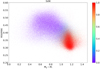 |
Fig. 3. Diagram of color indices g − i and inverse concentration indexes R50/R90 of 316 031 galaxies at z < 0.1 from the SDSS DR9 after applying the support-vector machine (SVM) method: red for early E types (from elliptical to lenticular) and blue for late L types (from S0a to irregular Im/BCG). The color bar from 0 to 1 shows the SVM probability to classify galaxy as late to early morphological types. |
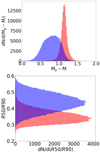 |
Fig. 4. Distribution of the morphological types (early in red, late in blue) in dependence on the color indices Mg − Mi (top) and inverse concentration index R50/R90 (bottom) for the main sample of 316 031 galaxies as in Fig. 3. |
The verification of the methods whether there are enough galaxies in a training sample to build a machine learning model is demonstrated in Fig. 5.
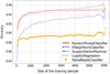 |
Fig. 5. Verification of whether there are enough galaxies in a training sample to build a machine learning model. The green line (support-vector machine), the red line (random forest), the pink line (logistic regression), the blue line (k-nearest neighbors), and the orange line (naive Bayes) show the average accuracy of ten repetitions of the evaluation procedure in Scikit-learn machine learning with Python. |
The results obtained for each method’s ability to accurately determine the morphological type of the galaxy can be easily illustrated graphically (Fig. 6). We consider the probability of finding the position of each galaxy (point on the graph) on the hyper-plane of two parameters (inverse concentration index and one of the color indices) for each of the used machine learning methods (Table 1). In each of the panels in Fig. 6 the input data from the training sample is embedded as in Fig. 1 (6163 galaxies randomly selected with different redshifts and luminosity from the SDSS DR9): red corresponds to the early morphological type, blue to the late-type galaxies. This visualization helps to analyze a tuning of the studied machine learning algorithms to classify the galaxy types.
 |
Fig. 6. Probability distribution for finding the position of each galaxy on the hyper-plane of two photometric parameters R50/R90 vs. Mg − Mi. The training sample (Fig. 1) is embedded in each of the panels, which shows the effectiveness of the methods used to classify galaxy types at z < 0.1. The accuracy of each applied machine learning method for the two-parameter classification is written in the left corner of each panel. |
5. Discussion
Various machine learning methods are helpful not only for the classification of objects by morphological features of celestial bodies. They are sufficient for reconstruction of the Zone of Avoidance (Vavilova et al. 2018), finding gamma-ray sources for the upcoming Cherenkov Telescope Array (Bieker 2018), spatio-temporal data (Wang et al. 2019), classification of variable stars light curves (Kim & Bailer-Jones 2016) and light-curve shape of a Type Ia supernova (Stahl et al. 2020), determination of the distance modulus for local galaxies (Elyiv et al. 2020) and photometric redshift estimation (Mu et al. 2020), prediction of galaxy halo masses (Calderon & Berlind 2019), gravitational lenses search (Khramtsov et al. 2019a), automating discovery and classification of variable stars (Bloom et al. 2012), and for analyzing huge observational surveys, for example the Zwicky Transient Facility (Mahabal et al. 2019), or finding planets and exocomets from the Kepler and TESS surveys (Kohler 2018).
Among other recent examples, we also note the determination of physical properties of galaxies (density, metallicity, column density, ionization) from their emission-line spectra with support-vector machine algorithms employed and developed in a new GAME numerical code by Ucci et al. (2017); prediction of the HI content of massive galaxies at z < 2 based on optical photometry data (SDSS) and environmental parameters, which was performed by Rafieferantsoa et al. (2018) with regressors and deep neural network (see also examples of applications of the AstroML Python module 5 for the large-scale observational extragalactic surveys3). In addition to the traditional approach for classifying the galaxy types automatically in the optical range, the machine learning methods also demonstrate a strong utility for classifying the radio galaxy types and peculiarities (Aniyan & Thorat 2017; Alger et al. 2018; Wagner et al. 2019; Lukic et al. 2019; Ralph et al. 2019).
When implementing machine learning methods for different astronomical tasks it is very useful to discuss their advantages and problem points, data quality regularity, and flexibility of the classification pipeline.
5.1. Several problem points of the supervised machine learning methods and data quality for the automated morphological classification of galaxies from the SDSS
The main problems of machine learning related to the morphological classification can be divided into two categories. The first concerns a sample preparation, which includes determining the parameters that are the best for dividing objects into classes, selecting a homogeneous data set for classification parameters, creating a sub-directory for training algorithms, cleaning the sublist of undesired (misclassified) objects, determining the most effective methods for the decision making, and selecting the best machine learning features to build training sample. The second category includes problems related to the individual peculiarities of selected objects and the quality of the image, the photometry, and the spectrum galaxy data.
Selection of the best parameters of machine learning for training. To determine the training parameters, we need the relationship between the model’s accuracy in training and test samples. In other words, we must choose parameters in such a way that (a) the accuracy of the test sample is as high as possible, (b) the accuracy of the methods applied to the training sample should not attain 100% value to avoid overfitting (see, e.g., the figures on the prediction accuracy by Vasylenko et al. 2019), and (c) the difference in accuracy between the test and training samples is minimal. However, these requirements do not always coincide simultaneously. So, the averaged values of the training and test samples’ accuracy ratios should be analyzed for a larger number of cycles to determine the best parameters.
To select the optimal parameters, we applied the GridSearchCV tool from the Scikit-learn library and the balanced class scales for the classifiers, except for the Gaussian naive Bayes. The balanced mode in models uses the values to automatically adjust the weights, which are inversely proportional to the input data’s class frequencies.
Features of galaxies, which are the best fitted for the morphology classification into types. To determine these photometry parameters, we need (a) to create a small homogeneous galaxy sample for training, where all the data sets have certain types available in the database; (b) to test these parameters using, for example, the Fisher method for evaluating the significance of these features (Fig. 7); and (c) to determine the distribution of galaxies of different types at different redshifts selecting sets of benchmarks by analyzing slices for one or several parameters.
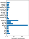 |
Fig. 7. Estimation of the relative importance of some photometric parameters for the random forest classifier of galaxies from the SDSS. The training sample contains 11 000 galaxies. Parameters with the highest values correspond to the most significant parameters: deVABu, deVABg, deVABr, deVABi, deVABz for the de Vaucouleurs radius fit b/a in different bands; expABu, expABg, expABr, expABi, expABz for the exponential fit b/a in different bands; z for redshift; Mu − Mr, Mg − Mi, Mr − Mz for the color indices; Mu, Mg, Mr, Mi, Mz for the absolute magnitudes, and R50/R90 for the inverse concentration index to the center. |
We can see in Fig. 7 that the higher relative importance among photometric parameters, which correlate with morphology, have the color indices Mu − Mr, Mg − Mi, Mr − Mz, and inverse concentration index to the center R50/R90. Other features such as absolute magnitudes Mu, Mg, Mr, Mi, Mz; exponential fits b/a in different bands expABu, expABg, expABr, expABi, expABz; de Vaucouleurs radius fits b/a in different bands deVABu, deVABg, deVABr, deVABi, deVABz; and redshift z are less important. We verified that inclusion of exponential fits, de Vaucouleurs radius fits, and redshifts as the additional features of galaxies does not increase the accuracy of machine learning methods applied to the training sample of 11 301 galaxies. This is 83.6% when they are also included (see Table 2 for SVM classifier). We did not use them, and this allowed us to also reduce the computational cost.
Accuracy (in %) of the supervised machine learning methods for the automated binary morphological classification (total, for early E and late L morphological types, rms error) of modified training sample of 11301 galaxies from the SDSS DR9 at z < 0.1 (region with the overlap of types in Figs. 1 and 3).
Image–photometry–spectrum quality of the data. The examples of images of galaxies, which are correctly classified into early and late types, are given in Fig. 8. The problem points of the SDSS galaxy data, which led to their morphology misclassification, are as follows (Fig. 9): (1) interacting galaxies (Fig. 9a), (2) background galaxy (Fig. 9b), (3) stars covering the galaxy image (Fig. 9c), (4) artifacts (diffraction, satellites) (Fig. 9d), (5) red spiral galaxies or 6) galaxies with a bright nucleus (Fig. 9f), (7) bad background, (8) dim objects (low signal-to-noise ratio), (9) face-on and edge-on galaxies (Figs. 9g, h), and 10) “false” objects, such as gravitational lenses. (Fig. 9e). These objects can be simply identified and deleted at the step of building the finest quality training sample (see Sect. 2.2).
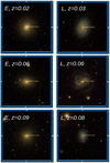 |
Fig. 8. Examples of images of galaxies from the SDSS DR9 at z < 0.1 classified correctly as early E and late L types. |
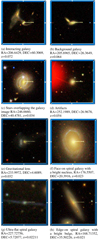 |
Fig. 9. Examples of images of galaxies from the SDSS DR9 at z < 0.1, when the morphological types can be misclassified in the machine learning pipeline. |
We also used the spectra in combination with image and photometry data in several questionable cases for the face-on spirals, lenticulars, and E0-E1 type galaxies to train classifiers (for instance, SDSS J124332.66+172004.3, SDSSJ155947.57+263334.4). Nevertheless, we conclude that such morphologically misclassified objects contribute ∼1% error in the classification of a general galaxy sample (see also Kasivajhula et al. 2007).
Human labeling (HL) was the only way to determine the morphological types of galaxies until the advent of the big data era (see, e.g., references on the early and modern galaxy surveys and catalogs in our review Vavilova et al. 2020b).
Among the works with 100% successful visual inspection that led to the discovery and cataloging of galaxies with types that do not fit into classical morphological schemes are on the interacting galaxies, galaxies with excess radiation in certain spectral ranges, compact galaxies, galaxies of low and high surface brightness, and others. For example, the use of the catalogs of galaxies of low surface brightness (dwarfs and normal) based on visual inspection, even in the absence of data on redshifts, made it possible to determine their role in the large-scale structure of normal galaxies in the Local Supercluster (see, e.g., Karachentseva & Vavilova 1994, 1995; Lisker et al. 2008; Miskolczi et al. 2011; Paudel et al. 2018).
Even though visual inspection of galaxies is becoming prohibitively time-consuming, the human labeling method remains a necessary classifier of morphological types both when compiling small samples of galaxies for solving various astrophysical and astrochemical tasks (Pilyugin et al. 2018; Du et al. 2019; Martin et al. 2020), and for building the training samples in tasks of automated classification.
Under these circumstances, we paid special attention to the labeling and cross-validation of the same galaxies from the training sample. As we mentioned in Sect. 2.2, it was performed by the authors.
At the same time, following works by Willett et al. (2013), Kuminski & Shamir (2016), and Beck et al. (2018) mentioned in the Introduction, we compared our results and the debiased GZoo2 data trying to take into account all the differences in approach to the labeling of morphological features of galaxies.
With this aim, we cross-matched 316 031 galaxies and their morphological types obtained by the support-vector machine with the GZoo2 data, which yielded ∼173 000 galaxies (SVM and GZoo2 in Fig. 10). The accuracy is 69.7%. We also cross-matched 6 163 galaxies from the training sample (HL in Fig. 10) with the GZoo2 data, which yielded 4834 common galaxies. The accuracy is 72.2%. The coordinate error for cross-matching in both cases is dRA, Dec ≤ 1″.
 |
Fig. 10. Confusion matrices after cross-matching of the studied samples and GZoo2: HL – 4834 galaxies from training sample; SVM – ∼173 000 galaxies with the support-vector machine classifier: E, early-type galaxies; L, late-type galaxies; green, galaxies that have the same type in both samples; red, galaxies where the types did not match. |
The similarity of accuracy values indicates, first of all, that both support-vector machine and human labeling manage equally well when we use the photometry-based approach to compare our binary classification with the GZoo2 data. Second, the Fig. 10 highlights a different approach to the visual labeling of galaxies by morphological types for our galaxy sample and the GZoo2 sample. The confusion matrices allow us to understand the differences in this labeling: the left panel demonstrates to what extent our visual classification (HL) of galaxies from the training sample coincides with the GZoo2 classification; the right panel gives information to what extent the automated classification with the support-vector machine (SVM) coincides with the GZoo2 classification. The percentage of the samples that do not coincide is about 30% in both cases.
For this reason, we decided to determine the main photometric parameters used in our work (color indices Mg − Mi and inverse concentration index R50/R90) for the ∼173 000 matched galaxies from the GZoo2. We can see in Figs. 11 and 12 that the dispersion in the data of the GZoo2 sample is more extensive compared with our studied sample (Fig. 2). First of all, there is a strong asymmetry by the photometric parameters: the bimodality in distribution of early (red) and late (blue) morphological types for our sample (Fig. 2) and the blur in distribution by types (no bimodality) for the GZoo2 data (Fig. 12). Secondly, there is a bigger overlap of the early- and late-type galaxies. This asymmetry confirms that galaxies of the same type were labeled differently in the two samples.
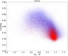 |
Fig. 11. Distribution of ∼173 000 galaxies at z < 0.1 from the GZoo2 on the plane of photometric parameters of color indices g − i and inverse concentration indexes R50/R90: early (red) and late (blue) morphological types are from the GZoo2 labeling. |
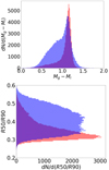 |
Fig. 12. Distribution of the morphological types (early, red; late, blue) in dependence on the photometric parameters: color indices Mg − Mi (top) and inverse concentration index R50/R90 (bottom) for the GZoo2 sample of ∼173 000 galaxies, as in Fig. 11. |
To analyze this case we selected randomly 5% of the 173 000 matched galaxies (∼8500) and applied the support-vector machine classifier to this GZoo2 sample. We used the morphological types labeled by GZoo2 volunteers and photometric parameters adopted in our study. The obtained accuracy is 76%. As can be seen in Fig. 11, the GZoo2 morphological classification is not as efficient when we apply our photometric criteria (Sect. 2.1 and Fig. 7). The drop in the accuracy can arise due to the inconsistency regarding human labeling in our classification and that of GZoo2. One of the partial reasons can be the attribution of irregular galaxies in GZoo2, which have redder color indices, to the elliptical (early-type) galaxies, and vice versa, elliptical galaxies with the bluer color indices to the spiral (late-type) galaxies.
The detailed comparison of these features is not the purpose of this article; however, this labeling bias means that we cannot get an accuracy significantly exceeding 76% when we use the GZoo2 data as a training sample for machine learning with the photometry-based approach.
We find that the morphology based on the supervised machine learning methods trained over photometric parameters demonstrates significantly less bias than morphology based on citizen-science classifiers. This conclusion is in agreement with the results by Cabrera-Vives et al. (2018), who found that “this result holds even when there is underlying bias present in the training sets used in the supervised machine learning process”.
5.2. Comparison of the supervised machine learning methods for the automated morphological classification of galaxies
Accuracy of the methods as a function of redshift. We estimated the prediction of galaxy morphological type in dependence on the redshift by five supervised machine learning techniques.
We tested the dependencies with equal binning δz = 0.008 by redshift and when each redshift bin contains the same number of galaxies (left and right panels, respectively, in Fig. 13). Each point in each bin in this figure shows the absolute number of coincident morphological types of galaxies at a given redshift interval.
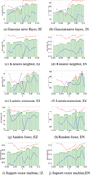 |
Fig. 13. Accuracy of each of the supervised machine learning methods to determine the morphological type of galaxies from the SDSS at z < 0.1 as a function of redshift (late type, blue; early type, red; averaged accuracy, green). Left panel: uniform binning by redshift (EZ) with δz = 0.008; right panel: each bin contains the same number of galaxies (EN). Only the tops of the histograms are shown. |
We can see in Fig. 13 that random forest and logistic regression give higher averaged accuracy (green lines) for all intervals of redshifts. Our calculations also demonstrate that random forest clearly gives the highest accuracy (95%) for the nearby galaxies (see Sect. 3.2). The support-vector machine and k-nearest neighbors have, on average, good results for all morphological types, on a par with the other supervised machine learning methods which have slightly higher accuracy of determining the early galaxy type for all intervals of redshifts than for the late galaxy type (see also tuning for all these methods in Fig. 6).
So, we did not find a dependence on the redshift for the accuracy of supervised machine learning methods to determine the morphological type of galaxies from the SDSS at z < 0.1. But it must be remembered that a well-formed representation of galaxies at all redshifts in the training sample plays a key role in the absence of this dependence.
The overlap of the types in range of Mg − Mi from 1.1 to 1.3. The aforementioned misclassification error related to the image–photometry–spectrum quality of the data (Sect. 5.1) is the same when we make a decision on how to recognize morphological types of galaxies in a region, where their photometry parameters are overlapping (see Fig. 1 for training and Fig. 3 for the main samples) in the region of Mg − Mi from 1.1 to 1.3. Should we select only morphologically well-defined objects to avoid visual classification errors? or add poorly classified objects in the hope of finding more subtle features for each morphological type?
To answer these questions we added ∼5000 galaxies from this region into the training sample. They were selected by the ability to determine a certain binary morphological type (50 ± 5%) with support-vector machine classifier. This allowed us to test accuracy changes and to define benefits from such a tuning (see also Fig. 6 for this method in a range of color indices from 1.0 to 1.3). We can see in Table 2 that such an approach worsened the accuracy results of the classification (for comparison, see Table 1). The reason is that the training sample becomes subjective depending on the human labeling rather than on the parameters for machine learning classifiers (see also Sect. 5.1 on human labeling).
Most of the galaxies with misclassified types are related to the bluer HI-rich galaxies of early-type galaxies (Fig. 14a) and to the redder HI-poor spiral galaxies (Fig. 14b, which are labeled as early type galaxy in GZoo2). As well, there are populations of HI-rich spirals having very red integrated colors indistinguishable from those for elliptical and lenticular galaxies (Schommer & Bothun 1983) and the so-called “anemic” (van den Bergh 1991) or “passive” spirals, which have spiral morphologies, but do not show star formation activity. For the latter case, we note the work by Goto et al. (2003) for a study of 25 813 SDSS galaxies at 0.05 < z < 0.1. These galaxies can be considered a transition population between early-type galaxies at low redshifts and late-type galaxies in higher redshift clusters (0.2 < z < 0.5). The population of such spirals with the high level of dust extinction is more numerous in these clusters (Bekki & Couch 2010). So, the major or minor mergers can influence the age distribution of stars making their red disks observable (see, e.g., Davidge et al. 2012 for an explanation of this case for spiral M31). In addition, the star formation in early-type galaxies determined in HI content (see Grossi et al. 2009; Nyland et al. 2017; Yıldız et al. 2020) causes their color indices to turn bluer in the optical range. So, only the spectral data may serve arbitrarily to distinguish these misclassified morphological types.
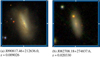 |
Fig. 14. Examples of the SDSS galaxies illustrating the overlap of the early and late morphological types: (left) NGC 2764 (lenticular), which is the HI-rich early-type galaxy; (right) HI-poor spiral galaxy (Sc type). (a) J090817.46+212636.0, z = 0.009026. (b) J082708.18+274837.6, z = 0.020330. |
Edge-on and face-on galaxies. We used the Revised Flat Galaxy Catalogue (RFGC) with 4444 galaxies (Karachentsev et al. 1999) and the Two-Micron Flat Galaxy Catalogue (2MFGC) with 18 020 galaxies (Mitronova & Korotkova 2015) (1) for cross-verification of the edge-on galaxies from our sample, which should be recognized as the late-type spirals and never as the ellipticals, and (2) for an analysis of a contribution of this error type into the accuracy of the applied machine learning methods. The RFGC gives the data on coordinates, axis ratio, position angles, and names of galaxies (including the names in the Principal Galaxy Catalogue; Paturel et al. 1989), but does not contain information on the radial velocities or redshifts. After cross-matching, our sample contains 934 flat galaxies from the RFGC as well as 3143 galaxies from the 2MFGC.
We estimated the accuracy of an edge-on galaxy to be classified as a late morphological type by five machine learning techniques and the multi-parametric method. We can see in Table 3 that random forest and logistic regression give the highest mean accuracy. More importantly, this accuracy is 86% for naive Bayes and 72% for logistic regression for edge-on galaxies at z ≤ 0.05 and ∼50% for random forest and support-vector machine at z > 0.05. As a result for these samples (galaxies from RFGC and 2MFGC), we conclude that all five machine learning techniques and multi-parametric diagrams provide the correctly classified edge-on types for 2/3 of the total samples of galaxies. This error is mostly related to the galaxies at very low redshifts (see Fig. 9h).
Accuracy for edge-on galaxies from the RFGC catalog to be classified as the late morphological types by the machine learning methods and multi-parametric diagram.
Edge-on galaxies are not the only ones that contribute errors in the accuracy of determining morphological type based on the photometric parameters. Some inconsistencies can also be explained by such factors as errors in determining the type of galaxies seen face-on (especially with a pronounced bulge, see Fig. 9f) or the evolutionary peculiarities of blue early-type galaxies (Fig. 14a). Altogether they complicate the biasing of results requiring more time for verification than the human labeling. For the first notice, we recommend a paper by Lingard et al. (2020), who developed a novel method, Galaxy Zoo Builder, which works well with face-on galaxy image modeling based on the four-component photometric decomposition of spiral galaxies. The second notice related to the transformation from disk to elliptical morphology of low redshift galaxies is well described by Schawinski et al. (2014), who used SDSS, GALEX, and GZ data.
A separate case of flat galaxies are the bulge-less (ultra-flat) galaxies with inclination 87 ° ÷90° for seen edge-on (Fig. 9g) and 10 ° ÷0° for seen face-on. One of the criteria is the major-to-minor diameter ratio in blue (a/b)B ≥ 7 (as for the RFGC, where the fraction of ultra-flat galaxies is ∼19%). We note that most of these galaxies look, on average, almost two times thinner in the Hα filter than those in the red continuum (Kaisin et al. 2020). A less stringent criterion (a/b)B ≥ 3 was used in compiling catalogs of SDSS galaxies with a bulge to super-thin ones (Kautsch et al. 2006; Bizyaev et al. 2014). The face-on bulge-less galaxies can be considered counterparts to the edge-on disk galaxies giving additional information on their parameters, including photometry, hidden by the projection effect. These objects can be correctly and easily classified as late-type spirals at the stage of training sample building.
At the same time, the results of applying the deep convolutional neural network to the images of our studied sample (Khramtsov et al. 2019b, 2020) with the same aim of a binary morphological classification have shown limitations. Specifically, deep learning methods can classify rounded sources as ellipticals, but it cannot catch the spectral energy distribution properties of galaxies more clearly than support-vector machine methods trained on the photometric features of galaxies.
Generally, we have overestimated the number of elliptical galaxies and underestimated the number of spiral galaxies when the face-on and edge-on galaxies are classified morphologically. This problem can be decided when we form training samples through several steps (pre-training, fine-tuning, and classification). The steps of fine-tuning include (1) limitations on the axes-ratio for elliptical galaxies, (2) additional photometry parameters for the face-on spiral galaxies to estimate the bulge-to-disk ratio, and (3) trainings with multi-band images and spectral features of galaxies.
6. Conclusions
We presented the results of the automated morphological classification of 316 031 galaxies from the SDSS with redshifts of 0.02 < z < 0.1 and absolute stellar magnitudes of −24m < Mr < −19.4m.
Using the visual classification of galaxies and multi-parametric diagrams color-Mr, color-R50/R90, color-deVRadr, and color-expRadr, we found prominent criteria for separating the galaxies into three classes: (1) early types, elliptical and lenticular; (2) spirals Sa − Scd, and (3) late spirals Sd − Sdm and irregular Im/BCG types. Due to a low accuracy for the Sa − Scd types of galaxies, we concentrated our exploration of the automated classification on two classes, E early and L late types of galaxies.
We evaluated the accuracy of different supervised machine learning methods to be applied to the binary automated morphological classification of galaxies (naive Bayes, random forest, support-vector machine, logistic regression, and k-nearest neighbors algorithm). To study the classifier, we used absolute magnitudes Mu, Mg, Mr, Mi, Mz; color indices Mu − Mr, Mg − Mi, Mu − Mgg, Mr − Mz; and the inverse concentration index to the center R50/R90. We paid special attention to the training sample building, which contains 2% of the main sample. To select the optimal parameters, we applied the GridSearchCV tool from the Scikit-learn library and the balanced class scales for the classifiers, except for the Gaussian naive Bayes. The balanced mode in the models uses the values to automatically adjust the weights, which are inversely proportional to the input data’s class frequencies. We proposed the visualization, which helps to analyze a tuning of the studied machine learning algorithms to classify galaxy types as a probability distribution in the hyper-plane of the selected photometric parameters.
We obtained that methods of support-vector machine and random forest with the Scikit-learn software machine learning library in Python provide the highest accuracy for the binary galaxy morphological classification with the photometry-based approach. We found a success rate of 96.4% for support-vector machine (96.1% early E and 96.9% late L types) and 95.5% for random forest (96.7% early E and 92.8% late L types).
This allowed us to create a catalog of morphological types of 316 031 galaxies from the SDSS at z < 0.1. Applying the support-vector machine, we revealed 139 659 E-type and 176 372 L-type galaxies among them.
We cross-matched 316 031 galaxies and their morphological types obtained by the support-vector machine with the GZoo2 data, which yielded ∼173 000 galaxies. The morphological types labeled by GZoo2 volunteers were gone with our photometry-based approach and demonstrated a labeling bias. The bimodality distribution by color indices was a key principle in our study. We concluded that the GZoo2 as a training sample for machine learning with the photometry-based main parameters cannot provide accuracy significantly exceeding 76%. So, the morphology based on the supervised machine learning methods trained over photometric parameters demonstrates significantly less bias than morphology based on citizen-science classifiers.
We verified the dependencies of the accuracy of supervised machine learning methods on the redshift, data quality, human labeling bias (including the cases of edge-on and face-on galaxies), and overlap of different morphological types for galaxies with the same color indices.
We did not find a dependence of the supervised machine learning accuracy to predict galaxy morphological type on the redshift. But it must be remembered that for the absence of this dependence, a well-formed representation of galaxies at all redshifts in the training sample plays a key role. We checked the overlap of the early and late galaxy types in range of Mg − Mi from 1.1 to 1.3 for the studied sample and found that the prediction of types becomes subjective depending on the human labeling rather than on the parameters for machine learning classifiers. Most galaxies with misclassified types are related to the bluer HI-rich galaxies of early-type galaxies and to the redder HI-poor spiral galaxies.
An analysis of problem points showed that support-vector machine and random forest are effective tools for the automated galaxy morphology classification based on the photometric parameters. Moreover, it once again confirmed that when the relationships between the parameters for classification the more complex, the more flexible model should be applied.
The image-based similarity learning approach with the use of a convolutional neural network trained on the images of galaxies from the studied sample matched in the GZoo2 data set will be presented in our next paper by Khramtsov et al. (2020).
Acknowledgments
We thank Prof. Massimo Capacciolli and Dr. Valentina Karachentseva for the fruitful discussion and remarks. We are grateful to the referee for useful comments that allowed us to present the results of our study more fully. This work was supported in frame of the budgetary program “Support for the development of priority fields of scientific research”? (CPCEL 6541230), the grant for Young Scientist’s Research Laboratories (2018–2019, Dobrycheva D.V.), and the Youth Scientific Project (2019–2020, Dobrycheva D.V., Vasylenko M.Yu.) of the National Academy of Sciences of Ukraine. The use of the SDSS (Ahn et al. 2012; Blanton et al. 2017; Ahumada et al. 2020), HyperLeda (Makarov et al. 2014), and SAO/NASA Astrophysics Data System was extensively applicable. This study has also made with the NASA/IPAC Extragalactic Database (NED), which is operated by the Jet Propulsion Laboratory, California Institute of Technology, under contract with the NASA.
References
- Ahn, C. P., Alexandroff, R., Allende Prieto, C., et al. 2012, ApJS, 203, 21 [Google Scholar]
- Ahumada, R., Prieto, C. A., & Almeida, A. 2020, ApJS, 249, 3 [Google Scholar]
- Al-Jarrah, O. Y., Yoo, P. D., Muhaidat, S., Karagiannidis, G. K., & Taha, K. 2015, ArXiv e-prints [arXiv:1503.05296] [Google Scholar]
- Alger, M. J., Banfield, J. K., Ong, C. S., et al. 2018, MNRAS, 478, 5547 [Google Scholar]
- Andrae, R., Melchior, P., & Bartelmann, M. 2010, A&A, 522, A21 [EDP Sciences] [Google Scholar]
- Aniyan, A. K., & Thorat, K. 2017, ApJS, 230, 20 [Google Scholar]
- Ball, N. M., & Brunner, R. J. 2010, Int. J. Mod. Phys. D, 19, 1049 [Google Scholar]
- Ball, N. M., Loveday, J., Fukugita, M., et al. 2004, MNRAS, 348, 1038 [Google Scholar]
- Balogh, M. L., Baldry, I. K., Nichol, R., et al. 2004, ApJ, 615, L101 [Google Scholar]
- Banerji, M., Lahav, O., Lintott, C. J., et al. 2010, MNRAS, 406, 342 [Google Scholar]
- Barchi, P. H., de Carvalho, R. R., Rosa, R. R., et al. 2020, Astron. Comput., 30 [Google Scholar]
- Beck, M. R., Scarlata, C., Fortson, L. F., et al. 2018, MNRAS, 476, 5516 [CrossRef] [Google Scholar]
- Bekki, K., & Couch, W. J. 2010, MNRAS, 408, L11 [Google Scholar]
- Bieker, J. 2018, Am. Astron. Soc. Meet. Abstr., 232, 220.03 [Google Scholar]
- Bizyaev, D. V., Kautsch, S. J., Mosenkov, A. V., et al. 2014, ApJ, 787, 24 [Google Scholar]
- Blanton, M. R., Bershady, M. A., Abolfathi, B., et al. 2017, AJ, 154, 28 [NASA ADS] [CrossRef] [Google Scholar]
- Bloom, J. S., Richards, J. W., Nugent, P. E., et al. 2012, PASP, 124, 1175 [Google Scholar]
- Breiman, L. 2001, in Machine Learning, ed. P. Flach, 5 [Google Scholar]
- Burkov, A. 2019, in The Hundred-Page Machine Learning Book, 152 [Google Scholar]
- Buta, R. J. 2011, ArXiv e-prints [arXiv:1102.0550] [Google Scholar]
- Cabrera-Vives, G., Miller, C. J., & Schneider, J. 2018, AJ, 156, 284 [Google Scholar]
- Calderon, V. F., & Berlind, A. A. 2019, MNRAS, 490, 2367 [NASA ADS] [CrossRef] [Google Scholar]
- Cheng, T.-Y., Conselice, C. J., Aragón-Salamanca, A., et al. 2020, MNRAS, 493, 4209 [Google Scholar]
- Chilingarian, I. V., & Zolotukhin, I. Y. 2012, MNRAS, 419, 1727 [Google Scholar]
- Chilingarian, I. V., Melchior, A.-L., & Zolotukhin, I. Y. 2010, MNRAS, 405, 1409 [NASA ADS] [CrossRef] [Google Scholar]
- Conselice, C. J., Bluck, A. F. L., Mortlock, A., Palamara, D., & Benson, A. J. 2014, MNRAS, 444, 1125 [Google Scholar]
- Cortes, C., & Vapnik, V. 1995, in Machine Learning, ed. P. Flach, 273 [Google Scholar]
- Davidge, T. J., McConnachie, A. W., Fardal, M. A., et al. 2012, ApJ, 751, 74 [Google Scholar]
- de la Calleja, J., & Fuentes, O. 2004, MNRAS, 349, 87 [Google Scholar]
- Dobrycheva, D., & Melnyk, O. 2012, Adv. Astron. Space Phys., 2, 42 [Google Scholar]
- Dobrycheva, D. V. 2013, Odessa Astron. Publ., 26, 187 [Google Scholar]
- Dobrycheva, D. V. 2017, Ph.D. Thesis, Main Astronomical Observatory, NAS of Ukraine [Google Scholar]
- Dobrycheva, D. V., Melnyk, O. V., Vavilova, I. B., & Elyiv, A. A. 2015, Astrophysics, 58, 168 [Google Scholar]
- Dobrycheva, D. V., Vavilova, I. B., Melnyk, O. V., & Elyiv, A. A. 2018, Kinematics Phys. Celestial Bodies, 34, 290 [Google Scholar]
- Du, W., Cheng, C., Wu, H., Zhu, M., & Wang, Y. 2019, MNRAS, 483, 1754 [Google Scholar]
- El Bouchefry, K., & de Souza, R. S. 2020, in Learning in Big Data: Introduction to Machine Learning, eds. P. Škoda, & F. Adam, 225 [Google Scholar]
- Elyiv, A. A., Melnyk, O. V., Vavilova, I. B., Dobrycheva, D. V., & Karachentseva, V. E. 2020, A&A, 635, A124 [EDP Sciences] [Google Scholar]
- Fluke, C. J., & Jacobs, C. 2020, WIREs Data Mining and Knowledge Discovery, 10 [Google Scholar]
- Gauthier, A., Jain, A., & Noordeh, E. 2016, AJ, 149, 1 [Google Scholar]
- Goto, T., Okamura, S., Sekiguchi, M., et al. 2003, PASJ, 55, 757 [Google Scholar]
- Grossi, M., di Serego Alighieri, S., Giovanardi, C., et al. 2009, A&A, 498, 407 [NASA ADS] [CrossRef] [EDP Sciences] [Google Scholar]
- Ivezic, E. D., Babu, G. J., & Challenges, Statistical 2014, Astronomy, 1 [Google Scholar]
- Ivezic, Z., Connolly, A. J., VanderPlas, J. T., & Gray, A. 2014, in Statistics, Data Mining, and Machine Learning in Astronomy: A Practical Python Guide for the Analysis of Data, eds. Z. Ivezic, A. J. Connolly, J. T. VanderPlas, & A. Gray, 559 [Google Scholar]
- Kaisin, S. S., Karachentsev, I. D., Hernandez-Toledo, H., Gutierrez, L., & Karachentseva, V. E. 2020, Astrophys. Bull., 75, 1 [Google Scholar]
- Karachentsev, I. D., Karachentseva, V. E., Kudrya, Y. N., Sharina, M. E., & Parnovskij, S. L. 1999, Bull. Spec. Astrophys. Obs., 47, 5 [Google Scholar]
- Karachentseva, V. E., & Vavilova, I. B. 1994, Bull. Spec. Astrophys. Obs., 37, 98 [NASA ADS] [Google Scholar]
- Karachentseva, V. E., & Vavilova, I. B. 1995, Kinematics Phys. Celestial Bodies, 11, 38 [Google Scholar]
- Kasivajhula, S., Raghavan, N., & Shah, H. 2007, MNRAS, 8, 1 [Google Scholar]
- Kates-Harbeck, J. 2012, APS April Meeting Abstracts, 2012, E1.075 [Google Scholar]
- Kautsch, S. J., Grebel, E. K., Barazza, F. D., & Gallagher, J. S. I. 2006, A&A, 445, 765 [NASA ADS] [CrossRef] [EDP Sciences] [Google Scholar]
- Khramtsov, V., Dobrycheva, D., Vasylenko, M., et al. 2020, A&A, submitted [Google Scholar]
- Khramtsov, V., Sergeyev, A., Spiniello, C., et al. 2019a, A&A, 632, A56 [EDP Sciences] [Google Scholar]
- Khramtsov, V., Dobrycheva, D. V., Vasylenko, M. Y., & Akhmetov, V. S. 2019b, Odessa Astron. Publ., 32, 21 [Google Scholar]
- Kim, D.-W., & Bailer-Jones, C. A. L. 2016, A&A, 587, A18 [NASA ADS] [CrossRef] [EDP Sciences] [Google Scholar]
- Kohler, S. 2018, Using Machine Learning to Find Planets (AAS Nova Highlights) [Google Scholar]
- Kremer, J., Stensbo-Smidt, K., Gieseke, F., Steenstrup Pedersen, K., & Igel, C. 2017, IEEE Intell. Syst., 32, 16 [Google Scholar]
- Kuminski, E., & Shamir, L. 2016, ApJS, 223, 20 [Google Scholar]
- Lahav, O., Naim, A., Sodre, L., & Storrie-Lombardi, M. C. 1995, MNRAS, 283, 207 [Google Scholar]
- Lahav, O., Naim, A., Sodré, L., Jr, & Storrie-Lombardi, M. C. 1996, MNRAS, 283, 207 [Google Scholar]
- Lingard, T. K., Masters, K. L., Krawczyk, C., et al. 2020, ApJ, 900, 178 [Google Scholar]
- Lintott, C. J., Schawinski, K., Slosar, A., et al. 2008, MNRAS, 389, 1179 [NASA ADS] [CrossRef] [Google Scholar]
- Lisker, T., Grebel, E. K., & Binggeli, B. 2008, AJ, 135, 380 [Google Scholar]
- Lukic, V., Brüggen, M., Mingo, B., et al. 2019, MNRAS, 487, 1729 [Google Scholar]
- Mahabal, A., Rebbapragada, U., Walters, R., et al. 2019, PASP, 131 [Google Scholar]
- Makarov, D., Prugniel, P., Terekhova, N., Courtois, H., & Vauglin, I. 2014, A&A, 570, A13 [CrossRef] [EDP Sciences] [Google Scholar]
- Martin, G., Kaviraj, S., Hocking, A., Read, S. C., & Geach, J. E. 2020, MNRAS, 491, 1408 [Google Scholar]
- Melnyk, O. V., Dobrycheva, D. V., & Vavilova, I. B. 2012, Astrophysics, 55, 293 [Google Scholar]
- Miskolczi, A., Bomans, D. J., & Dettmar, R. J. 2011, A&A, 536, A66 [NASA ADS] [CrossRef] [EDP Sciences] [Google Scholar]
- Mitronova, S. N., & Korotkova, G. G. 2015, Astrophys. Bull., 70, 24 [Google Scholar]
- Mittal, A., Soorya, A., Nagrath, P., & Hemanth, D. J. 2020, Earth Sci. Inform., 13, 601 [Google Scholar]
- Mu, Y.-H., Qiu, B., Zhang, J.-N., Ma, J.-C., & Fan, X.-D. 2020, Res. Astron. Astrophys., 20, 089 [Google Scholar]
- Murrugarra, J., & Hirata, N. 2017, SIBGRAPI2017 e-proceedings, 1 [Google Scholar]
- Naim, A., Lahav, O., Sodre, L. J., & Storrie-Lombardi, M. C. 1995, MNRAS, 275, 567 [Google Scholar]
- Nair, P. B., & Abraham, R. G. 2010, ApJS, 186, 427 [Google Scholar]
- Nyland, K., Young, L. M., Wrobel, J. M., et al. 2017, MNRAS, 464, 1029 [Google Scholar]
- Paturel, G., Fouque, P., Bottinelli, L., & Gouguenheim, L. 1989, A&AS, 80, 299 [Google Scholar]
- Paudel, S., Smith, R., Yoon, S. J., Calderón-Castillo, P., & Duc, P.-A. 2018, ApJS, 237, 36 [Google Scholar]
- Pedregosa, F., Varoquaux, G., Gramfort, A., et al. 2011, J. Mach. Learn. Res., 12, 2825 [Google Scholar]
- Pilyugin, L. S., Grebel, E. K., Zinchenko, I. A., et al. 2018, A&A, 613, A1 [NASA ADS] [CrossRef] [EDP Sciences] [Google Scholar]
- Rafieferantsoa, M., Andrianomena, S., & Davé, R. 2018, MNRAS, 479, 4509 [Google Scholar]
- Rahman, W. M. A., & Azhari, S. 2018, Int. J. Adv. Res. Sci. Eng. Technol., 5, 6066 [Google Scholar]
- Ralph, N. O., Norris, R. P., Fang, G., et al. 2019, PASP, 131 [Google Scholar]
- Raschka, S. 2015, in Python Machine Learning, ed. R. Banerjee, 1 [Google Scholar]
- Schawinski, K., Urry, C. M., Simmons, B. D., et al. 2014, MNRAS, 440, 889 [Google Scholar]
- Schlegel, D. J., Finkbeiner, D. P., & Davis, M. 1998, ApJ, 500, 525 [NASA ADS] [CrossRef] [Google Scholar]
- Schommer, R. A., & Bothun, G. D. 1983, AJ, 88, 577 [Google Scholar]
- Simmons, B. D., Lintott, C., Willett, K. W., et al. 2017, MNRAS, 464, 4420 [Google Scholar]
- Sreejith, S., Pereverzyev, S. J., Kelvin, L. S., et al. 2018, MNRAS, 474, 5232 [Google Scholar]
- Stahl, B. E., Martínez-Palomera, J., Zheng, W., et al. 2020, MNRAS, 496, 3553 [Google Scholar]
- Storrie-Lombardi, M. C., Lahav, O., Sodre, L. J., & Storrie-Lombardi, L. J. 1992, MNRAS, 259, 8P [Google Scholar]
- Ucci, G., Ferrara, A., Gallerani, S., & Pallottini, A. 2017, MNRAS, 465, 1144 [Google Scholar]
- van den Bergh, S. 1991, PASP, 103, 390 [Google Scholar]
- VanderPlas, J. 2016, in Python Data Science Handbook: Essential Tools for Working with Data, ed. D. Schanafelt, 1563 [Google Scholar]
- VanderPlas, J., Connolly, A. J., Ivezic, Z., & Gray, A. 2012, Proceedings of Conference on Intelligent Data Understanding (CIDU), 47 [Google Scholar]
- Vasylenko, M. Y., Dobrycheva, D. V., Vavilova, I. B., Melnyk, O. V., & Elyiv, A. A. 2019, Odessa Astron. Publ., 32, 46 [Google Scholar]
- Vavilova, I. B., Melnyk, O. V., & Elyiv, A. A. 2009, Astron. Nachr., 330, 1004 [Google Scholar]
- Vavilova, I. B., Ivashchenko, G. Y., Babyk, I. V., et al. 2015, Kosmichna Nauka i Tekhnologiya, 21, 94 [Google Scholar]
- Vavilova, I. B., Elyiv, A. A., & Vasylenko, M. Y. 2018, Russ. Radio Phys. Radio Astron., 23, 244 [Google Scholar]
- Vavilova, I., Dobrycheva, D., Vasylenko, M., Elyiv, A., & Melnyk, O. 2020a, in Multiwavelength Extragalactic Surveys: Examples of Data Mining, eds. P. {\v{S}}koda, & F. Adam, 307 [Google Scholar]
- Vavilova, I., Pakuliak, L., & Babyk, I. 2020b, in Surveys, Catalogues, Databases, and Archives of Astronomical Data, ed. P. Škoda, & F. Adam, 57 [Google Scholar]
- Wagner, S., Melnik, V., & Rucker, H. 2019, in EPSC-DPS Joint Meeting 2019, 2019 EPSC-DPS2019-751 [Google Scholar]
- Wang, S., Cao, J., & Yu, P. S. 2019, ArXiv e-prints [arXiv:1906.04928] [Google Scholar]
- Way, M. J., Scargle, J. D., Ali, K. M., & Srivastava, A. N. 2012, Advances in Machine Learning and Data Mining for Astronomy (Taylor& Francis Group: CRC Press) [Google Scholar]
- Willett, K. W., Lintott, C. J., Bamford, S. P., et al. 2013, MNRAS, 435, 2835 [Google Scholar]
- Yıldız, M. K., Peletier, R. F., Duc, P. A., & Serra, P. 2020, A&A, 636, A8 [EDP Sciences] [Google Scholar]
- York, D. G., Adelman, J., Anderson, J. E., et al. 2000, AJ, 120, 1579 [CrossRef] [Google Scholar]
All Tables
Accuracy (in %) of the supervised machine learning methods for the automated binary morphological classification of galaxies from the SDSS DR9 at z < 0.1 (total, for early E and late L morphological types, rms error)
Accuracy (in %) of the supervised machine learning methods for the automated binary morphological classification (total, for early E and late L morphological types, rms error) of modified training sample of 11301 galaxies from the SDSS DR9 at z < 0.1 (region with the overlap of types in Figs. 1 and 3).
Accuracy for edge-on galaxies from the RFGC catalog to be classified as the late morphological types by the machine learning methods and multi-parametric diagram.
All Figures
|
Fig. 1. Diagram of color indices g − i and inverse concentration indexes R50/R90 of the training sample (6163 galaxies randomly selected with different redshifts and luminosities from the SDSS DR9). The visually classified galaxies (human labeling) of early E − S0 types are shown in red, and the late Sa − Irr types in blue. |
| In the text | |
|
Fig. 2. Distribution of the morphological types (early in red, late in blue) depending on the photometric parameters: (left panel) color indices Mg − Mi, (right panel) inverse concentration index R50/R90) for the training sample of 6163 galaxies as in Fig. 1. |
| In the text | |
|
Fig. 3. Diagram of color indices g − i and inverse concentration indexes R50/R90 of 316 031 galaxies at z < 0.1 from the SDSS DR9 after applying the support-vector machine (SVM) method: red for early E types (from elliptical to lenticular) and blue for late L types (from S0a to irregular Im/BCG). The color bar from 0 to 1 shows the SVM probability to classify galaxy as late to early morphological types. |
| In the text | |
|
Fig. 4. Distribution of the morphological types (early in red, late in blue) in dependence on the color indices Mg − Mi (top) and inverse concentration index R50/R90 (bottom) for the main sample of 316 031 galaxies as in Fig. 3. |
| In the text | |
|
Fig. 5. Verification of whether there are enough galaxies in a training sample to build a machine learning model. The green line (support-vector machine), the red line (random forest), the pink line (logistic regression), the blue line (k-nearest neighbors), and the orange line (naive Bayes) show the average accuracy of ten repetitions of the evaluation procedure in Scikit-learn machine learning with Python. |
| In the text | |
|
Fig. 6. Probability distribution for finding the position of each galaxy on the hyper-plane of two photometric parameters R50/R90 vs. Mg − Mi. The training sample (Fig. 1) is embedded in each of the panels, which shows the effectiveness of the methods used to classify galaxy types at z < 0.1. The accuracy of each applied machine learning method for the two-parameter classification is written in the left corner of each panel. |
| In the text | |
|
Fig. 7. Estimation of the relative importance of some photometric parameters for the random forest classifier of galaxies from the SDSS. The training sample contains 11 000 galaxies. Parameters with the highest values correspond to the most significant parameters: deVABu, deVABg, deVABr, deVABi, deVABz for the de Vaucouleurs radius fit b/a in different bands; expABu, expABg, expABr, expABi, expABz for the exponential fit b/a in different bands; z for redshift; Mu − Mr, Mg − Mi, Mr − Mz for the color indices; Mu, Mg, Mr, Mi, Mz for the absolute magnitudes, and R50/R90 for the inverse concentration index to the center. |
| In the text | |
|
Fig. 8. Examples of images of galaxies from the SDSS DR9 at z < 0.1 classified correctly as early E and late L types. |
| In the text | |
|
Fig. 9. Examples of images of galaxies from the SDSS DR9 at z < 0.1, when the morphological types can be misclassified in the machine learning pipeline. |
| In the text | |
|
Fig. 10. Confusion matrices after cross-matching of the studied samples and GZoo2: HL – 4834 galaxies from training sample; SVM – ∼173 000 galaxies with the support-vector machine classifier: E, early-type galaxies; L, late-type galaxies; green, galaxies that have the same type in both samples; red, galaxies where the types did not match. |
| In the text | |
|
Fig. 11. Distribution of ∼173 000 galaxies at z < 0.1 from the GZoo2 on the plane of photometric parameters of color indices g − i and inverse concentration indexes R50/R90: early (red) and late (blue) morphological types are from the GZoo2 labeling. |
| In the text | |
|
Fig. 12. Distribution of the morphological types (early, red; late, blue) in dependence on the photometric parameters: color indices Mg − Mi (top) and inverse concentration index R50/R90 (bottom) for the GZoo2 sample of ∼173 000 galaxies, as in Fig. 11. |
| In the text | |
|
Fig. 13. Accuracy of each of the supervised machine learning methods to determine the morphological type of galaxies from the SDSS at z < 0.1 as a function of redshift (late type, blue; early type, red; averaged accuracy, green). Left panel: uniform binning by redshift (EZ) with δz = 0.008; right panel: each bin contains the same number of galaxies (EN). Only the tops of the histograms are shown. |
| In the text | |
|
Fig. 14. Examples of the SDSS galaxies illustrating the overlap of the early and late morphological types: (left) NGC 2764 (lenticular), which is the HI-rich early-type galaxy; (right) HI-poor spiral galaxy (Sc type). (a) J090817.46+212636.0, z = 0.009026. (b) J082708.18+274837.6, z = 0.020330. |
| In the text | |
Current usage metrics show cumulative count of Article Views (full-text article views including HTML views, PDF and ePub downloads, according to the available data) and Abstracts Views on Vision4Press platform.
Data correspond to usage on the plateform after 2015. The current usage metrics is available 48-96 hours after online publication and is updated daily on week days.
Initial download of the metrics may take a while.