| Issue |
A&A
Volume 648, April 2021
|
|
|---|---|---|
| Article Number | A42 | |
| Number of page(s) | 18 | |
| Section | Extragalactic astronomy | |
| DOI | https://doi.org/10.1051/0004-6361/202038260 | |
| Published online | 09 April 2021 | |
High angular resolution polarimetric imaging of the nucleus of NGC 1068
Disentangling the polarising mechanisms
1
LESIA, Observatoire de Paris, PSL Research University, CNRS, Sorbonne Universités, UPMC Univ. Paris 06, Univ. Paris Diderot, Sorbonne Paris Cité, 5 Place Jules Janssen, 92190 Meudon, France
e-mail: This email address is being protected from spambots. You need JavaScript enabled to view it.
2
SOFIA Science Center, USRA, NASA Ames Research Center, Moffett Field, CA 94035, USA
3
Université de Strasbourg, CNRS, Observatoire Astronomique de Strasbourg, UMR 7550, 67000 Strasbourg, France
4
Research School of Astronomy and Astrophysics, Australian National University, Canberra, ACT 2611, Australia
5
Université Côte d’Azur, Observatoire de la Côte d’Azur, CNRS, Laboratoire Lagrange, Bd de l’Observatoire, CS 34229, 06304 Nice Cedex 4, France
6
ETH Zurich, Institute for Particle Physics and Astrophysics, Wolfgang-Pauli-Strasse 27, 8093 Zurich, Switzerland
7
Institute of Astronomy, KU Leuven, Celestijnenlaan 200D B2401, 3001 Leuven, Belgium
8
Univ. Grenoble Alpes, CNRS, IPAG, 38000 Grenoble, France
9
Aix Marseille Université, CNRS, CNES, LAM, Marseille, France
10
NOVA Optical Infrared Instrumentation Group, Oude Hoogeveensedijk 4, 7991 PD Dwingeloo, The Netherlands
11
DOTA, ONERA, Université Paris Saclay, 91123 Palaiseau, France
Received:
24
April
2020
Accepted:
16
December
2020
Abstract
Context. Polarisation is a decisive method to study the inner region of active galactic nuclei (AGNs) since, unlike classical imaging, it is not affected by contrast issues. When coupled with high angular resolution (HAR), polarisation can help to disentangle the location of the different polarising mechanisms and then give insight into the physics taking place in the core of AGNs.
Aims. We obtained a new data set of HAR polarimetric images of the archetypal Seyfert 2 nucleus of NGC 1068 observed with SPHERE/VLT. We aim in this paper to present the polarisation maps and to spatially separate the location of the polarising mechanisms, thereby deriving constraints on the organisation of the dust material in the inner region of this AGN.
Methods. With four new narrow-band images between the visible and the near-infrared combined with older broad-band observations, we studied the wavelength dependence of the polarisation properties from 0.7 to 2.2 μm of three selected regions within the inner 2″ surrounding the central engine. We then compared these measurements to radiative transfer simulations of scattering and dichroic absorption processes, using the Monte Carlo code MontAGN.
Results. We establish a detailed table of the relative importance of the polarising mechanism as a function of aperture and wavelength. We are able to separate the dominant polarising mechanisms in the three regions of the ionisation cone, the extended envelope of the torus, and the very central bright source of the AGN. Thus, we estimate the contribution of the different polarisation mechanisms to the observed polarisation flux in these regions. Dichroic absorption is estimated to be responsible for about 99% of the polarised flux coming from the photo-centre. However, this contribution would only be restricted to this location because the double-scattering process would be the most important contributor to polarisation in the equatorial plane of the AGN and single scattering is dominant in the polar outflow bi-cone.
Conclusions. Even though results are in good agreement with larger apertures measurements, the variety of situations with different mechanisms at play highlights the importance of spatial resolution for the interpretation of polarisation measurements. We also refine the estimation of the integrated optical depth in the visible of the obscuring structure to a range of 20−100, constraining the geometry of the inner region of this AGN.
Key words: galaxies: Seyfert / galaxies: individual: NGC 1068 / techniques: high angular resolution / techniques: polarimetric / methods: numerical / methods: observational
© L. Grosset et al. 2021
 Open Access article, published by EDP Sciences, under the terms of the Creative Commons Attribution License (https://creativecommons.org/licenses/by/4.0), which permits unrestricted use, distribution, and reproduction in any medium, provided the original work is properly cited.
1. Introduction
As a consequence of the continuous progress of instrumentation, our understanding of the organisation of the centre of active galactic nuclei (AGNs) has been growing rapidly in the last few years. In particular, we are now resolving the core of nearby AGNs at an unprecedented parsec size spatial scale owing to the development of high angular resolution (HAR) techniques, in particular interferometry and extreme adaptive optics (AO), with the help of polarisation. Recent ALMA observations of two of the closest and brightest AGNs, NGC 1068 (García-Burillo et al. 2016, 2019; Imanishi et al. 2018, 2020; Lopez-Rodriguez et al. 2020; Impellizzeri et al. 2019) and Circinus (Izumi et al. 2018), resolved the molecular material surrounding the central engine (CE) at different frequencies. The associated dust of the CE is thought to block the light emitted when observing the nucleus edge on, as proposed years ago by Antonucci & Miller (1985), Antonucci (1993). Using the GRAVITY interferometer (at VLTI), the GRAVITY Collaboration (2018) was able to constrain the shape of the broad-line region of nearby quasar 3C 273 to a rotating thick disc and identified the sublimation region in NGC 1068 (GRAVITY Collaboration 2020). Finally, this view is completed owing to the high-contrast imaging coupled with polarimetry, as shown for instance by Packham et al. (1997, 2007) and Lopez-Rodriguez et al. (2015) with different instruments in the near to mid infrared range (Gratadour et al. 2015; Grosset et al. 2018).
Polarimetric imaging is less affected by contrast issues because polarisation provides more measurable intrinsic parameters of the light than just its intensity, namely the two parameters describing the orientation of the linear polarisation and, for some instruments, the circular polarisation. Therefore, by looking at the polarisation of the incoming light, we can access information on the material responsible for the polarisation, either by scattering, absorption, or emission, even in the vicinity of bright sources. Polarisation has revealed itself to be a very efficient method to study media close to a very bright source typical of the environments of AGNs, as demonstrated by Antonucci & Miller (1985), using polarised light to detect broad lines in the spectrum of NGC 1068.
The model of the obscuring material surrounding the CE has been undergoing evolution, from a simple torus shape in the early 1990s (Antonucci 1993) to the current complex, clumpy, and dynamical environments such as those modelled by Izumi et al. (2018). Identifying the mechanism responsible for the polarisation in AGNs provides information on the nature and characteristics of the scatterers. Several phenomena can be responsible for polarisation, principally scattering on dust grains or on electrons (Antonucci & Miller 1985) or dichroic absorption or emission by elongated dust grains (Efstathiou et al. 1997; Lopez-Rodriguez et al. 2015).
As concerns the mechanisms giving rise to polarisation, single scattering is currently observed in the polarisation of circum-stellar environments, such as by Kervella et al. (2015) with SPHERE/ZIMPOL (VLT, ESO’s Paranal Observatory). More complex signatures have also been invoked in young stellar objects, such as the double scattering process presented by Bastien & Menard (1990) and simulated by Murakawa (2010). This mechanism is also thought to be present in the outer envelope of the obscuring material of AGNs (Grosset et al. 2018) to account for the observed polarisation in the 20 × 60 pc central region (Gratadour et al. 2015).
Dichroism is expected to induce polarisation closer to the very central core of AGN. For elongated grains to emit or absorb photons with a preferential polarisation orientation, a mechanism that is responsible for aligning these grains on a large enough scale is required (Efstathiou et al. 1997), typically on few parsecs size in the case of AGNs (Lopez-Rodriguez et al. 2015). The magnetic field has been a promising candidate for aligning dust grains and the measured polarisation can then be used to constrain magnetic field properties, as achieved recently by Lopez-Rodriguez et al. (2015).
In recent years, there have been a growing number of simulation works to better understand the physics of AGNs through polarisation properties. These works include Nenkova et al. (2002), Alonso-Herrero et al. (2011), Marin et al. (2015), Lopez-Rodriguez et al. (2015), Grosset et al. (2018). The importance of polarisation in the understanding of AGNs has also been revealed by the large quantity of polarimetric measurements on the AGN of NGC 1068, the archetypal Seyfert 2 galaxy (D ≈ 14 Mpc), at all wavelengths in the last 50 years; these were compiled by Marin (2018a).
Concerning this AGN, Antonucci & Miller (1985) first invoked scattering as the mechanism responsible for the polarisation, as it would scatter the light emitted in the broad-line region, hidden by the torus, above the equatorial plane towards the observer. There have been ongoing discussions about the nature of the scatterers between electrons and dust grains. Antonucci (1993) favoured electrons due to the observed independence of the polarisation with wavelength. Polarimetric observations by Packham et al. (1997) in the near-infrared (NIR) confirmed the location of scatterers in the polar region of NGC 1068 and it is now expected that both electrons and dust grains are populating this region. Packham et al. (2007) and Lopez-Rodriguez et al. (2016) detected polarisation in the narrow-line region around 10 μm, which was most likely produced by dichroic emission by dust, while Marin et al. (2015) combined both electrons and dust grains populations in their simulations to study the polar outflows. Scattering on dust grains has now been observed on NGC 1068 at medium spatial scales (Gratadour et al. 2015, at about 100 to 200 pc).
We obtained new polarimetric HAR images of NGC 1068 thanks to SPHERE (installed at the Nasmyth focus of the UT3, Melipal, of the VLT, at ESO’s Paranal Observatory) in three narrow bands (NB) in the NIR and one in the visible. In this paper, we present the data sets and discuss the evolution of the polarisation in the different observed structures in the inner region as a function of wavelength to constrain the polarising mechanisms. We detail in Sect. 2 these new observations, and the obtained polarimetric maps. We then present, in Sect. 3, the polarisation as a function of wavelength in different selected regions of the AGN. In Sect. 4, we detail how dichroism was introduced in the numerical simulations conducted using our code MontAGN. We compare in the observations to the simulations in Sect. 5. We then discuss this comparison and the new insight brought by these new observations in Sect. 6 before concluding.
2. Observations and data processing
2.1. Observations summary
This study is based on three data sets of the central region of the Seyfert 2 galaxy NGC 1068, obtained in polarimetric mode at HAR with the instrument SPHERE (Beuzit et al. 2008) at VLT, ESO Paranal Observatory. The first data are those of the SPHERE science verification (SV) observing programme, obtained in H and Ks bands with the sub-module IRDIS (Dohlen et al. 2008; Langlois et al. 2014), published and analysed in Gratadour et al. (2015) and Grosset et al. (2018). The second set was observed between the 11 and 14 September 2016, with the IRDIS system as well, bringing three additional NBs polarimetric images in the NIR, namely Continuum H, Continuum K1, and Continuum K2 (hereafter Cnt H, Cnt K1, and Cnt K2, respectively). Filters properties can be found in Table 1. As for the first data set, the bright nucleus was used as a guide source for the SPHERE extreme adaptive optics system SAXO (Fusco et al. 2006), giving a correction quality comparable to what was achieved in the SV observation; SAXO could not be used at full capacity in both observations due to flux limitation. Seeing was comparable to the previous run, ranging between 0.7 and 1.2″; a complete summary is available in Table 1. Investigations into the radial profile of the central peak in all five NIR bands by Rouan et al. (2019) show no clear modification of the point spread function (PSF; see their Fig. 4), which could indicate a change in the resolution, and the achieved angular resolution is estimated to 60 mas (i.e. 4 pc at 15 Mpc).
Log of the SPHERE observations (IRDIS and ZIMPOL).
NGC 1068 was also observed with ZIMPOL, another SPHERE sub-system (Schmid et al. 2018) on 12 October 2016, in the frame of the Other Science SPHERE guaranteed time observation (GTO), adding the narrow-band NR (narrow red, in the visible at 645.9 nm, see Table 1 for filter characteristics) to the available polarimetric data. Similar to the IRDIS observations, SAXO was used but because of a lack of photons, no information about the achieved angular resolution could be retrieved. The SPHERE system aimed at estimating the AO efficiency, SPARTA is known to suffer bias in the case of faint targets, and this information is thus not reliable, as described in Milli et al. (2017), highlighted in their Fig. 2. The seeing was comparable to those of IRDIS and we expect the AO correction to be similar, with lower achieved resolution due to the wavelength dependence on the AO correction. The achieved resolution can be estimated around 100−150 mas based on the smallest structure detectable on the ZIMPOL image. A summary of the observations is presented in Table 1.
Owing to the increasing importance of sky emission, it is usual to match the sky observation integration time to the on-target integration time when observing in the NIR. However, because of the specific data processing of dual polarimetric imaging, we do not need sky acquisitions for each half-wave plate (HWP) position in polarimetric measurements, as shown in Table 1. More details about the polarimetric sky subtraction strategy will be developed in an upcoming paper.
2.2. Data reduction
The ZIMPOL polarimetric maps (0.0036″ per pixel, Schmid et al. 2018) were created using the official SPHERE-ZIMPOL pipeline. Maps of total and polarised intensities, degree of linear polarisation and angle of linear polarisation are shown in Fig. 1.
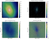 |
Fig. 1. Maps of intensity (in log10(ADU/s), upper left panel), polarised intensity (in log10(ADU/s), upper right panel), linear degree of polarisation (in %, lower left panel), and linear angle of polarisation (in degrees, lower right panel) in NR (645.9 nm) with ZIMPOL. North is up and east is to the left. |
All IRDIS polarimetric images (from both observing runs) were reduced with the same dedicated pipeline including sky subtraction, flat-field correction, and realignment after a median filter of size 3 × 3 pixels2. The eight final images were then realigned precisely before being combined using the inverse matrix method1, as described in Appendix A, to produce the intensity and polarisation Q and U maps; IRDIS records two images with perpendicular polarisation at the same time. As detailed in Sect. 3.4 and Appendix C, Cnt K2 (2266 nm) images were selected to avoid depolarisation due to the SPHERE derotator.
From these obtained maps, we finally transformed the images into polarised intensity Iplin, linear polarisation degree Plin, and linear polarisation position angle θlin maps (polarisation position angle reference follows IAU 1973 recommendations, starting from north and counting positive from north to east) following
 (1)
(1)
 (2)
(2)
and
 (3)
(3)
respectively.
Maps were then corrected from distortion and true north orientation. The images were shrunk along the vertical axis by a factor 1.006 and rotated using the orientation of the true north as measured by Maire et al. (2016) of −1.75°. Final NB maps, for IRDIS, with pixels of 0.01225″ (more precisely evolving between 0.012251″ and 0.012265″ per pixel, from the H to K band, according to Maire et al. 2016) for the total and polarised intensities, degree of linear polarisation, and the linear angle of polarisation are shown in Figs. 2–4.
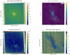 |
Fig. 2. Maps of intensity (in log10(ADU/s), upper left panel), polarised intensity (in log10(ADU/s), upper right panel), linear degree of polarisation (in %, lower left panel), and linear angle of polarisation (in degrees, lower right panel) in Cnt H (1573 nm). Polarisation vectors have been over-plotted to the polarised intensity maps of upper right panel, with a length relative to the local polarisation degree. A reference length for a 5% vector is shown. North is up and east is to the left. |
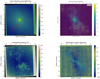 |
Fig. 3. Same as Fig. 2 for Cnt K1 (2091 nm). The red arrows indicate the position of the two south-western arcs. |
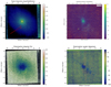 |
Fig. 4. Same as Fig. 2 for Cnt K2 (2266 nm). The red arrows indicate the position of the two south-western arcs. |
3. Polarisation in selected areas
As shown in Figs. 2–4, the Cnt H (1573 nm) and Cnt K1 (2091 nm) polarimetric maps harbour the same structures as already identified by Gratadour et al. (2015) on broad H and Ks bands (1625 and 2182 nm, respectively). Namely, we identified a highly polarised (5 to 10%) central source surrounded by a well-defined, polarised, hourglass-shaped region tracing the double ionisation cones and two low polarisation regions on the perpendicular direction to the hourglass axis at the level of the waist (north-west and south-east), interpreted as a signature of the obscuring material (Gratadour et al. 2015; Grosset et al. 2018). The Cnt K2 (2266 nm) maps share some common points with the previous two wavelengths, the polarised central source is also present, although less polarised, and the low polarisation region have a similar extension. However these maps also show some differences because the hourglass-shaped structure is identified on the polarised intensity map, but this structure is harder to distinguish on the polarisation degree and angle maps and the polarisation angle maps show a rather different behaviour. These peculiarities are discussed in Sect. 3.4.
With a smaller field of view (FOV) of only 3.6″ × 3.6″, the ZIMPOL NR (645.9 nm) image is to be compared with the central region of the NIR maps (FOV of 11″ × 12.5″). In the polarisation degree map, we recognise the elongated north-south structure seen in the inner 1″ of the NIR maps, but no other structure can be identified.
To investigate the properties of the different identified structures with respect to the wavelength, we extracted the global polarimetric signal from several peculiar regions in the four NBs and the two broad bands (BB). We focus on three important regions: the two south-western arcs laying between 1.5 and 2.5″ from the photo-centre, within the ionisation cone; the very central region at the photo-centre; and the low polarisation double region surrounding the central source in the south-east and north-west directions between 0.5 and 1.5″ from the centre.
3.1. Polarisation uncertainty
One major effect to be taken into account when measuring polarisation within aperture is the impact of the size of the aperture on the measured polarisation. It is expected (see Table 2 of Lopez-Rodriguez et al. 2016; Marin 2018a for polarisation dependence on the aperture size in NGC 1068) that the larger the aperture is, the smaller the polarisation degree owing to both increasing dilution by non-polarised light and the inclusion of differently polarised light within the aperture. This later effect is especially important in this work since we do see clear differences at small scales between regions in the inner 2″ of the AGN, in particular between the very central region, the low polarisation region and the south-western arcs. One major advantage of HAR in polaro-imaging is to better resolve the polarised emission.
As discussed in Tinbergen (1996), it is difficult to evaluate the quality of polarimetric maps. The signal-to-noise ratio (S/N) for example is not defined well since a higher intensity does not correspond to a higher degree of polarisation. Furthermore, when the degree of polarisation is small, neither the polarisation angle nor the polarisation degree follow Gaussian distributions.
We thus used two different methods, detailed in Appendix B, to evaluate the uncertainty on our polarisation measurements. In our apertures, this uncertainty generally ranges between 15 and 20% (see error bars in the following figures).
3.2. South-western arcs
The two south-western arcs, identifiable around 2″ south-west of the central source, are detected in all the NIR polarisation maps and directly on the intensity map of Cnt K1 and Cnt K2 (2091 and 2266 nm, respectively). We extracted the polarisation in eight regions, of size 0.2″ × 0.2″2, from east to west along each of the arcs. A zoom on the two arcs and the apertures used in this work are shown in Fig. 5. The aperture measurements are based on extraction of signal on the I, Q, and U maps, translated onto final polarimetric parameters using Eqs. (1) and (3). The error bars are based on the “pseudo-noise” approach of Eq. (B.1). The measured polarisation degree and polarisation position angle for all filters are shown in Fig. 6.
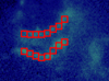 |
Fig. 5. Position of the apertures along the two arcs, south-west from the central source, on top of a polarisation degree map in H (1.6 μm). |
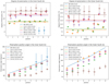 |
Fig. 6. Degree (in %, first row) and angle (in degrees, second row) of polarisation as a function of position in the arc, from east to west, for the inner south-western arc (first column) and the outer south-western arc (second column), for all the observing bands (colour coded). Average value of the polarisation degree in a given band is indicated by the respective colour horizontal lines. Second row: the blue line corresponds to the expected polarisation position angle for these apertures if due to single scattering of light coming from the photo-centre of the AGN. |
The first row of Fig. 6 shows that the degree of linear polarisation (shown versus a position offset in this figure) in the south-western structures tends to increase as a function of wavelength in all apertures. This is illustrated in Fig. 7, which represents the evolution of the averaged degree of polarisation as a function of wavelength in both arcs. We note that they evolve on a very similar linear increase, which is an evidence that an unique mechanism is responsible for the polarisation in the two arcs. Furthermore, the degree of polarisation, always higher in the outer arc, might suggest a scattering geometry configuration closer to 90° for this arc.
 |
Fig. 7. Degree of polarisation (in %), averaged for all 8 apertures in both arcs (colour coded) as a function of wavelength. |
The polarisation position angle, indicated in the second row of Fig. 6, is consistent with the expected variation for a centro-symmetric pattern, which is computed as the orthogonal direction to the photo-centre for every aperture position. Cnt K2 (2266 nm) is the most divergent from this pattern and this case is discussed in Sect. 3.4. We note however that there is a trend, which is stronger for the outer south-western arc, for the measured polarisation position angles to be offset by up to 20°, that is below the expected angles. There are multiple possible reasons for this offset and they are difficult to disentangle. An offset between the emission centre of the scattered light and the reference centre of the image (the photo-centre in NIR) would produce an offset, but this offset should not depend on wavelength. A better explanation would be the addition of a slightly different polarisation orientation all along the extension of the arcs on the line of sight (LOS). Inclination of these arcs with respect to the plane of the sky would also introduce an offset in the polarisation since the polarisation angle would not be 90° in this case.
3.3. Central region
We analysed polarisation in the inner 2″ of the AGN in different apertures to properly interpret this complex region, where multiple polarisation mechanisms such as dichroic absorption by aligned elongated grains, Thomson scattering on electrons, and Mie scattering on dust grains may be in competition.
In particular, we analysed the very central 0.2″ (hereafter, “very centre”), encompassing the bright photo-centre, which shows a higher polarisation degree than in its immediate surroundings and a domination of the polarised flux. We also extracted polarisation from the very low polarisation regions surrounding this photo-centre, in the south-east and north-west directions, on the expected extension of the obscuring material (hereafter, “off centre”). We finally considered a large aperture of 1″ size (hereafter, the “central region”) to compare this study to other polarimetric investigations references of this region at larger scale. These apertures are identified in Fig. 8 and the measured polarisation degree and polarisation position angle, as a function of wavelength, are shown in Fig. 9.
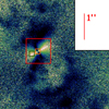 |
Fig. 8. Position and size of the apertures used for polarimetric measurements, superimposed to the differential polarisation angle map of BB H (1625 nm, from Gratadour et al. 2015). The orange aperture corresponds to the very centre, the green to the off-centre, and the red to the central region as described in text. |
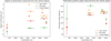 |
Fig. 9. Degree (in %, left panel) and angle (in degrees, right panel) of polarisation as a function of wavelength (in nm) for the three apertures in the central region of NGC 1068. Very centre refers to the very inner 0.2″, off-centre to the region with an offset on the torus extension direction, and central region to the large aperture integrating all the flux. See text of Sect. 3.3 for more details about these apertures. |
We also noted that, because the centre is very bright, the wings of the PSF of the central source could affect the innermost measurements. Because this central source is polarised, part of the measured polarisation could be contaminated by the higher polarisation from the centre, especially in the low polarisation regions. The PSF in the Ks (2182 nm) band for SPHERE, contributes up to 10% of the flux at ≈0.12″ from the centre, as shown with the same data by Rouan et al. (2019), for example by their Fig. 3, comparing the K profile to the PSF profile at K. This contribution of the central PSF then drops at larger distances. In particular, this implies that the polarisation degree contamination is smaller than 0.7% in Ks in the off centre aperture, which ranges between ≈0.2 and 0.4″ from the centre. As this PSF contribution is even smaller in H (1625 nm), we thus ensured that it does not significantly affect our measurements.
Figure 9 reveals very different trends for the three apertures. The large aperture central region has an almost linearly increasing polarisation degree from 1.5% to 4% between 0.7 μm and 2.2 μm (left panel), while the very centre and the off centre regions evolve in a less monotonic way. As expected, the off centre aperture represents the lower polarisation degrees, < 2%, with increases only at 2.0 μm to about 2−3%. In contrast, the very centre has a higher polarisation degree, starting at about 2% in R, increasing to a maximum of 5−7% at ≈1.6 μm and then decreasing to ≈4% at 2.2 μm.
As regards the polarisation position angle, it does not seem to undergo a noticeable evolution, for all apertures and wavelengths. Measurements range between 90 and 130°, encompassing the expected polarisation orientation in the central region in the NIR of ≈120° as measured by previous studies (Packham et al. 2007; Gratadour et al. 2015).
3.4. Case of Cnt K2
In most of the polarimetric maps and measurements in this work, Cnt K2 (2266 nm) results diverge from the other NIR results. In particular, Cnt K2 exhibits a rather different behaviour compared to the Cnt K1 and Ks filters, which are however at close wavelengths (2091 and 2182 nm, respectively). The Cnt K2 intensity map features a narrower central peak, leading to a lower flux in the surrounding of the very central peak. This limits the precision of polarimetric measurements since non-significant differences between Q and U maps at low S/N create random polarisation levels and, to some extent, explains these differences. These random polarisation levels outside the 1″ inner region pollutes the true polarised signal making its extraction more uncertain. We also note that the polarisation in the most central region is slightly lower in this band, even on the area not affected by this problem. The polarisation position angle is more problematic because it reveals very different patterns from other bands within regions shaped very similarly however. Both the polarisation position angle and degree are modified by a selection of the frames according to the SPHERE derotator position angle (see Appendix C for more details), and we thus investigate the effect of this on our polarimetric measurements in Appendix D.
Since both the binned polarisation degree and polarised intensity maps of Fig. D.1 reveal the features observed in the other NIR maps (especially the same polarisation degree of ≈15% in the south-western arcs), the difference in intensity is likely have the most impact on polarisation degree for this NB. Using the selection for raw images only leads to a lower S/N. Thus, our polarisation degree measurements should not be contaminated at a significant level by systematics coming from derotator depolarisation issues. However, binning of polarisation position angle map (Fig. D.1) does not lead to an improvement and an impact of the derotator position angle on the measured angle is very likely there. We thus do not go further into our investigations for this polarisation position angle map.
4. Simulation of dichroism
Grosset et al. (2018) succeeded in reproducing the constant polarisation position angle and low polarisation degree over the central region of NGC 1068 (about 20 × 60 pc) using the radiative transfer code MontAGN. This analysis was based on a double-scattering mechanism on spherical dust grains. The photons undergo two scattering events: one in the ionisation cone, where they are scattered back towards the equatorial plane, where in turn they are scattered a second time in the direction of the observer. These results are still in good agreement with the measurements in this paper. Especially, the overall polarisation position angle in the inner region and the low polarisation degree found in the south-east to north-west extension surrounding the very centre, are compatible with double scattering and therefore strengthen this interpretation. However, the relatively high (≈15%) polarisation degree of the photo-centre itself could not be explained by these simulations.
4.1. Framework
We extend this simulation work through simulations of polarimetric signal produced by dichroism. We used MontAGN (Grosset et al. 2018) to reproduce absorption of photons along a straight path through a region containing aligned elongated dust grains. As we aim to reproduce a signal observed between 0.5 μm and 2.3 μm, we focussed on dichroic absorption. At these wavelengths absorption is the dominant mechanism (Efstathiou et al. 1997) since temperature is expected to be high enough for a significant dust emission below 2.3 μm (i.e. above ≈400−500 K) only in the very inner region (≤1 pc) of the obscuring material and could thus be included in the central source. This emission would still have to suffer dichroic absorption by the rest of the colder dust structure surrounding it and has little impact on the final polarisation, even though it is possibly intrinsically polarised. If this effect is present, it would lower the dominant polarisation orientation flux, and thus slightly decrease the dilution fraction3 required to match the observed polarisation (see Sect. 4.3 for more details about dilution).
As MontAGN does not yet allow the user to align the orientation of the dust grains along a preferential direction, it is impossible to simulate dichroic absorption in the scattering framework of Grosset et al. (2018). We thus focussed on dichroism, which we investigated by simulating separately four polarisation orientation components (Q+, U+, Q−, and U−). For each of these, we set the dust properties to match the dust population encountered by this particular polarisation orientation. We then combined the output files to simulate the polarimetric properties of the resulting signal, generated only by dichroic absorption.
4.2. Producing dichroism signal
Following this method, we simulated polarimetric signals produced by dichroic absorption for a range of optical depth (τV ∈ [2.5, 200]) and for two different grain axis ratios. We used a ratio of major axis to minor axis of 1.5 (hereafter, “r1:1.5”) and a ratio of 2 (hereafter, “r1:2”). In both cases, we used a size distribution as in Mathis et al. (1977), with a power law of −3.5, ranging between 5 nm and 250 nm, with the variation depending on the axis ratios. Thus, for the first population, we used a distribution ranging between 5 nm and 125 nm for the minor axis and between 7.5 nm and 188 nm for the major axis. For the r1:2 population, we kept the same ratio for minor axis (between 5 and 125 nm) and set the major axis distribution between 10 nm and 250 nm. We show in this paper results for silicates dust grains, as simulations with graphites gave similar results. In a first step, photons packets were emitted using a flat spectrum4 between 0.5 and 3 μm and dust densities were set to match the chosen optical depth at 0.5 μm for each dust mixture integration.
Because elongated grains preferentially absorb photons polarised along their major axis, photons with different polarisation orientations do not encounter the same optical depth along their path through the same dust structure. For example, for our r1:1.5 model we get values of τV of 43.2, 6.8, and 25.0 along the Q+, Q−, and U± polarisation orientations, respectively, for an averaged τV = 25.0.
This difference of optical depth translates into different final fluxes for each of the polarisation orientations, thus creating a polarised signal. Simulated raw polarisation degree and polarised intensity spectra are shown in Fig. 10.
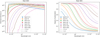 |
Fig. 10. Spectra of polarised intensity (first panel, with arbitrary intensity unit) and degree of polarisation (second panel) from dichroism simulated with MontAGN. |
Polarisation is very important at short wavelengths as shown by right panel of Fig. 10. At short wavelengths, only one of the polarisation orientation propagates significantly through the dust structure because of its optical depth (low fluxes, as shown by left panel), creating a 100% polarised signal. At longer wavelengths, the decrease of optical depth allows a fraction of the orthogonal polarisation to escape the obscuring material, and we thus observe a decrease in the polarised intensity and in the polarisation degree, especially for low optical depth models (where p ≈ 0, right panel).
4.3. Dilution
To compare our models with observations, we need to take into account additional effects. First, the flat spectrum used for emission needs to be adapted to our AGN case and we multiplied the output flux, after normalisation, by a typical emission spectrum. We used a simple source spectral energy distribution (SED) (see e.g., Siebenmorgen et al. 2015) based on Rowan-Robinson (1995) approximation for AGNs as follows:
 (4)
(4)
Polarised intensity and polarisation Q corrected spectra are shown in Fig. 11, for τV in the range 2.5−200 and for the two grain axis ratios. The Q polarisation spectrum (right panel) is the main polarisation indicator since we aligned the grain axis along the ±Q axis; photons with a ±U polarisation orientation encounter a 50/50 grain axis ratio mixture. Values of U do not exceed 0.0015 (0.15% of the maximum of the dichroic flux). The absolute value of polarisation Q evolution shows two phases. It first increases5 when the −Q photons, corresponding to the lowest optical depth, escape first and decrease when +Q photons are also able to escape. The polarised intensity graph (left panel) translates the same trends when weighted by total intensity.
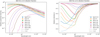 |
Fig. 11. Spectra of relative polarised intensity (first panel) and normalised polarisation Q intensity (second panel) for an AGN emission from MontAGN simulations. Polarised intensity is normalised to the maximum of the dichroic flux. |
In a second step, we need to properly account for dilution by all other emission sources contributing to the flux measured within the apertures. This is very critical since the high polarisation degree values in the left panel of Fig. 10 (at wavelength ≤1 μm) corresponds to very low fluxes (left panel) and is therefore reduced much more than the lower polarisation degree obtained at higher fluxes (at λ ≥ 1 μm).
We used a library of spectra compiled by Marin (2018b) for dilution. We used, similarly to this library, the compiled spectrum of a Sbc galaxy (see their Fig. 2), based on the morphological classification of NGC 1068, such as Balick & Heckman (1985). A proper spectrum then must be added to the computed intensity spectra, after scaling by dilution fraction, computed at 1 μm. Final SEDs and degree of polarisation are shown in Fig. 12 for dilution fractions of 0.5 and 0.8.
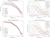 |
Fig. 12. Spectra of relative intensity (first column) and degree of polarisation (second column) for an AGN with dilution fractions of 50% (first row) and 80% (second row) from MontAGN simulations. Intensity is normalised to the maximum of the dichroic flux as detailed in text. |
The right column of Fig. 12 shows that dilution fraction and grain axis ratio have a similar affect on the polarisation degree spectrum in mostly changing the amplitude but not the overall shape of the curve. This implies that these two parameters are to some extent degenerated. We also note that the optical depth is the main parameter that drive the shape of the curve and thus is constrained in comparison with observations.
5. Comparison to observations
We computed fitting estimator maps as a function of optical depth and dilution fraction for both grain axis ratios. These maps, shown in Fig. 13, were obtained by computing the squared difference between the observed and simulated – through dichroism – polarisation degree for each data point, on the very central aperture. A comparison of the observed data with the best model curve for each grain axis ratio is shown in Fig. 14.
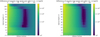 |
Fig. 13. Least-squares maps (in log scale) for r1:1.5 (left panel) and r1:2 (right panel) for dilution fraction varying between 0% and 100% (horizontal axis) and for optical depth τV between 2.5 and 200 (vertical axis). |
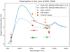 |
Fig. 14. Degree of polarisation (in %) as a function of wavelength (in nm) for both simulations and observations. The measurements are the same as in the first panel of Fig. 9 and represent the very centre in orange, the off-centre region in green, and the whole central region in red. The simulated spectra are shown in a continuous blue line for a grain ratio of 1:1.5 and dashed line for a ratio of 1:2, with corresponding optical depth and dilution fraction parameters to best fit the very-centre (orange) data points. |
5.1. Optical depth and dilution fraction
As shown in Fig. 13, the dilution fraction is constrained to a rather small range by the comparison between our observation and our simulations. Similarly, simulations also set a maximum and minimum limit values for the optical depth of the obscuring structure.
For the observed signal to be compatible with dichroic absorption, a dilution fraction of 60% to 85% is required, depending slightly on the optical depth and the grain axis ratio. Thus, the fraction of the total intensity received in the very central source of NGC 1068 through dichroism, and therefore directly coming from the CE, would be between 15% and 40% (at 1 μm), in rather good agreement with the ≈5% polarisation observed at the very centre between 1.5 μm and 2.3 μm.
The integrated optical depth of the structure is also constrained to values ranging between τV ≈ 20−100, slightly favouring values at the lower edge, with τV ≤ 50. Such dust densities would allow enough light to propagate through the obscuring material in the NIR in one of the polarisation orientations to create the observed dichroic polarisation. This constraint does not depend on the geometry or clumpiness of the medium. The obscuring material is very likely to be clumpy (see e.g., Marin et al. 2015), where the optical depth of individual clouds are currently estimated at 45 ≤ τV ≤ 115 for example by Lopez-Rodriguez et al. (2015), Audibert et al. (2017). Thus, our constraint would be compatible with an estimate of one to two clouds in our LOS to the CE.
5.2. Role of grain axis ratio
The other conclusion than can be driven from Fig. 13 is that even though the grain axis ratio impacts the optical depth difference between the two polarisation orientations, it does not translate into as large a difference in the measured polarisation degree. By comparing the two maps of Fig. 13, the difference introduced by a change in the grain axis ratio only slightly shifts both the required dilution fraction and the optical depth of the structure towards larger values. For instance, we measured for our second grain population a shift of ≈10% in the dilution fraction and an increase of ≈10 in the lower limit of the required optical depth in V.
We only tested two grain ratio populations with our simple model, with an orientation that is identical for all of the grains. It is expected (Efstathiou et al. 1997) that grains are not all perfectly aligned along the magnetic field and are precessing along the preferred orientation direction and that only a fraction of them are similarly orientated. Efstathiou et al. (1997) studied the impact of grain axis ratios and precession of the grains on the polarisation signal and concluded that the effect was small and comparable to a dilution of the signal, similar to what is shown in Fig. 13. This is consistent since a misalignment of part of the grain population would be modelled by a slightly different shape of grain.
5.3. Polarisation through scattering
These results correspond to an optical depth lower than that estimated by Grosset et al. (2018), who required τV ≈ 170 based on a double-scattering effect. However, this previous estimate used the polarimetric signal in all the central region (of 2″) of NGC 1068, thus including the very central emission. A high optical depth was therefore necessary to reproduce the polarimetric signal especially in this very central region, otherwise the unpolarised flux of the CE would mask the polarisation. However, if we consider that this central polarisation originates from dichroic absorption instead, we can lower the required optical depth and still produce double-scattering polarisation signal out of the very centre. We verified this assumption and Fig. 15 shows the polarimetric signal from scattering based on simulations developed in Grosset et al. (2018); for an optical depth of 45 in the V band. Polarisation pattern on the cone and an equatorial region of Fig. 15 are similar to those of the τV = 170 map of Grosset et al. (2018) and differ only on the central ≈3 pc. However, it is noteworthy that these two simulation works (Grosset et al. 2018; this work) were conducted using different frameworks of only spherical dust grains and only elongated dust grains, respectively. A full simulation framework would be required for a complete view of the mechanisms at the origin of the polarisation signal in the NIR and would be a very important extension of this work.
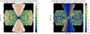 |
Fig. 15. Simulated map of polarisation degree (left) and polarisation position angle (right) computed by MontAGN for an integrated optical depth of τV = 45 along the equatorial LOS, with an inclination angle of 90° at 1.6 μm (without dichroism and without dilution). |
5.4. Effect on large apertures
Our polarisation measurements within the largest aperture (Fig. 14) are in fair agreement with the literature for similar or larger apertures. In particular, Fig. 9 shows an increasing trends between 500 nm and 2000 nm that fits well within the compilation of polarimetric measurements in Fig. 2 of Marin (2018a). This tends to confirm that our small aperture measurements are reliable and that we are separating different polarisation mechanisms in these two regions that become combined in larger apertures. In particular, we can distinguish at least three regions with different polarisation mechanisms: the very inner central spot dominated by dichroic absorption; the equatorial region of the off-centre region, ranging between few pc to ≈60 pc dominated by double scattering; and the bi-cone region between 60 and 200 pc in the polar directions dominated by single scattering.
6. Discussion
6.1. Global view
Owing to recent polarimetric studies (Gratadour et al. 2015; Lopez-Rodriguez et al. 2015; Grosset et al. 2018; Marin 2018a, this work), we propose a global scheme of the polarisation mechanisms in AGNs and in particular in NGC 1068. In the photo-centre, beyond 1 μm we would detect light coming directly from hot dust in the very inner region of the torus that is heated by the CE (Lopez-Rodriguez et al. 2015). Because of non-spherical grains more or less aligned by magnetic field, only one polarisation orientation preferentially propagates because the other is more absorbed, thereby creating the observed polarisation in the NIR at the very centre. Dichroism is the most likely polarising mechanism in this region since it is able to produce such high polarisation degrees (up to 15%) and a constant polarisation orientation. Beyond 2 μm, the optical depth becomes low enough for both the polarisation orientation to propagate through the material, leading to the observed decrease in the polarisation degree.
In the equatorial region, along the extension of the obscuring material, we detect a low polarisation that is likely to be produced by double scattering (Grosset et al. 2018) on a region centred on the photo-centre and extending to the equatorial direction to about 30 pc, with a 20 pc total thickness in the polar direction (Gratadour et al. 2015). This mechanism becomes negligible at the photo-centre because polarised flux becomes completely dominated by the effect of dichroic absorption at the photo-centre (the central PSF). The low polarisation signal is thus only detected at a location offset from the photo-centre.
Finally, in the polar directions, we detect a signal that can be explained by single scattering on material located in the double ionisation cone between few parsecs to about 200 pc. The origin of this scattering signal is possibly due to multiple species, depending on the location.
In the innermost regions, the material responsible for the scattering (see maps of Figs. 2–4 until 0.5″), zoomed on Fig. 16, is rather unclear. We observe an extension of the high polarisation degree along the polar direction in the H (1625 nm) and Ks (2182 nm) bands, as already stated by Gratadour et al. (2015), but also in the Cnt H (1573 nm) and K1 (2091 nm) polarisation maps. This feature is remarkably perpendicular to the CO structure detected on the central 10 pc with ALMA by García-Burillo et al. (2019), and could be due to electron scattering on the first 10 pc of the bi-cone, as invoked by Antonucci (1993) and observed by Antonucci et al. (1994) with the Hubble Space Telescope in the ultraviolet. But hot dust is known to be present in the polar outflow (Ramos Almeida & Ricci 2017, and references therein) and would also be a good candidate for scattering the light emitted by the CE. In both situations, it is expected that light emitted or scattered this close to the AGN centre would then cross through parts of the obscuring material, so that polarisation due to Thomson/Rayleigh/Mie scattering could be then combined with dichroic absorption by this material. As both of these effects in these regions are expected to produce polarisation with a similar position angle, it would be very difficult to disentangle the exact contribution of each of these mechanisms. As Thomson scattering on electrons is wavelength-independent, the main polarising mechanism is also likely to change between visible and IR close to the very centre, depending on the optical depth of the obscuring material.
 |
Fig. 16. Zoom on the polar extension of the detected polarisation degree, close to the very centre, on the Cnt K1 map (2.1 μm). Size of the image is ≈1.5 × 2″ and colour scale is the same as Fig. 3. |
At larger scales, dust grains are likely to be dominant. A comparison with ALMA data reveals that the southern arcs are very likely due to scattering on dusty material that is present in the ionisation cone and directly illuminated by the CE (García-Burillo et al. 2016, 2019).
As discussed in Sect. 5.4, depending on the size of the aperture used to measure the polarisation signal, different proportion of these – at least – three mechanisms must be used, thus leading to the differences between our measurements and the large aperture ones.
6.2. Relative importance of the mechanisms
Based on these measurements at HAR, we can attempt to estimate the relative contribution of these three mechanisms to the polarised intensity, as a function of their location.
As shown by Fig. 7, the degree of polarisation in the scattering region of the southern arcs is increasing with wavelength. This variation is both due to evolution in the polarised intensity, which slightly increases between H and Cnt K2 (from 1625 to 2266 nm); and to the global intensity, which strongly decreases at large distance from the centre with increasing wavelength (see upper panels of Figs. 2–4). This is mostly due to the decrease of the stellar emission in the inner few arcseconds between H and Ks (1625 and 2182 nm, respectively), as detailed in Rouan et al. (2019). A deeper study of the relation between the optical depth of the dust structures and the intensity and polarised intensity produced by this structure combined with data from ALMA would be a very interesting extension of this work.
In the equatorial region, which is offset from the photo-centre, the degree of polarisation is low and slightly increases towards 2.2 μm. This increase of the polarisation degree in Ks is most likely related to a decrease of the intensity as detailed in the previous paragraph. This is a stronger effect than what is observed in the southern arcs, the polarised intensity being quasi-constant in the equatorial region. This is consistent with the results of Grosset et al. (2018) on double scattering, which found a relatively constant low polarisation degree in the equatorial region (except in the very centre) regardless of the optical depth of the structure, as long as it is optically thick. This is the case since we would detect the centrosymmetric single scattering pattern if it were optically thin.
Combining these measurements, we estimated the contribution of dichroic absorption (versus scattering) to the polarised flux in the central region for different aperture sizes. The results are detailed in Table 2.
Contribution of dichroism to the polarised flux in different apertures for a given band (in %).
Thus according to Table 2, polarised intensity in the NIR, at the photo-centre, is expected to come at about 98% ± 1% from dichroic absorption. But interestingly, this contribution decreases to 50% and less at larger apertures, when more and more scattered flux fell within the aperture. This contribution increases with the wavelength because polarised flux in the Ks band is still dominated by dichroism even on a 3″ aperture. This ratio might be decreasing on the Cnt K2 band, around 2.3 μm, as the fraction is lowered to 38% ± 1%, however possible systematics do not allow us to reach a firm conclusion.
6.3. Geometry and optical depth of the dust structure
As stated in Sect. 5, our study tends to lower the estimation of the required optical depth along the LOS to the CE of the AGN derived by Grosset et al. (2018). This lower values originates from a reduced need to block the light directly coming from the centre, as polarisation is rather created by dichroic absorption (about 99%) than by double scattering (less than 2%) in the LOS. As discussed at the end of Grosset et al. (2018) and in Sect. 5 of the present work, dichroic absorption better reproduces the degree of polarisation at this location. We can thus set an upper value to the dust opacity at τV = 200 because if extinction is too high photons can barely escape the obscuring structure, which would be incompatible with a strong polarimetric signal produced by dichroic absorption (or any other mechanism). The range of optical depth of ≈20−100 in τV constrained by our model is consistent with what is generally expected for the obscuring structure of AGN (see e.g., Packham et al. 1997; Lopez-Rodriguez et al. 2015; Audibert et al. 2017; Rouan et al. 2019), lowering the previously estimation of Grosset et al. (2018).
We only simulated integrated absorption along the LOS to the CE in this work, and there is therefore no assumption on the geometry or nature (fragmentation) of the obscuring structure. In the ≈60 pc region of constant polarisation, the double-scattering process should still be involved and thus a dust density that decreases with the radius is still likely required to efficiently scatter photons (Grosset et al. 2018). Furthermore, this hypothesis is consistent with recent studies by Izumi et al. (2018), who developed a multi-phase dynamic torus model, with lower densities in the outer regions of the torus (R > 10 pc), based on ALMA observations of the Circinus galaxy.
We also resolved an elongation along the polar axis with a high polarisation degree in most of the NIR maps, close to the very centre, on a ≈10 pc scale. As discussed in Sect. 6.1, this could be due to scattering on electrons in the first parsecs of the ionisation cone or on hot dust in the outflow. What is surprising about this elongation is that both the polarisation degree and polarisation position angle are remarkably constant all along the structure, while the intensity undergoes large variations (thus reflected in the polarised flux) and while different mechanisms would be involved. We ask if it would be possible for two polarising effects (dichroism at the photo-centre and scattering on the polar extension encompassing the photo-centre) to be able to produce such similar polarisation. It is likely that dichroism also affects light scattered (or emitted) in the polar ionisation cone if close enough to the equatorial plane, since light would then have to cross through parts of the obscuring material. But we wonder where the transition between these two effects take place. Estimating the exact contribution of both phenomena to polarisation in this polar extension is thus difficult and would be an interesting study.
6.4. Magnetic field
Our estimation of the 98% to 99% contribution of the dichroic absorption to the polarised flux observed in the NIR is consistent with the assumption of Lopez-Rodriguez et al. (2015), who used a fraction of 100% to study the magnetic field in the central region of NGC 1068. Our measured polarisation degree in Ks (2182 nm) of 4.4% ± 0.2% is also in very good agreement with these measurement of 4.4 ± 0.1% by these authors. The optical depth range we estimated in this work, between 15 and 100 in the visible, corresponding to 1.7 to 12 in Ks, encompasses the value used by Lopez-Rodriguez et al. (2015) of τK ≈ 3.24, based on Packham et al. (1997). Having very similar values, we would derive an identical strength estimation for the magnetic field of 4 mG to 139 mG, as estimated by Lopez-Rodriguez et al. (2015). Our measurements also confirms that with HAR, the position angle for the polarisation orientation is very similar to those measured with larger apertures (Lopez-Rodriguez et al. 2015) and therefore reinforces the hypothesis of a toroidal geometry for the magnetic field (parallel to the polarisation position angle for dichroic absorption).
7. Conclusions and prospectives
We presented in this paper new observations of the core of the archetypal Seyfert 2 galaxy NGC 1068 in NB filters with the extreme adaptive optics instrument SPHERE. Our polarisation measurements within large apertures closely agree with the literature and fit the expected behaviour of the polarisation with wavelength well. However, by separating the signal in smaller apertures, owing to HAR imaging, we were able to trace rather different behaviours of polarisation regarding wavelength, depending on the location in the AGN environment, tracing as many different polarising mechanisms. Owing to these polarimetric measurements, combined with the previous polarisation maps in H and Ks (1625 and 2182 nm respectively), we investigated the properties of the following three major regions within the central 200 pc of the AGN and their associated dominant polarising mechanism:
-
The electrons and dust scattering in the ionisation cone, ranging between few tens of parsecs to ≈200 pc. In particular, the south-western arcs detected in the broad NIR bands by Gratadour et al. (2015) were re-observed and are compatible with single scattering, most likely on dust grains.
-
The dust double-scattering equatorial central region of the AGN, in which the first scattering would be in the polar region and the second in the equatorial region. This corresponds to constant polarisation orientation and degree on a 60 pc × 20 pc area, encompassing the photo-centre and tracing the outer envelope of the obscuring material (similarly to Grosset et al. 2018).
-
The dichroic absorption of the light, coming directly from the photo-centre of the AGN, from the CE.
Furthermore, we identified a fourth region, at the transition between the photo-centre and the ionisation cone up to ≈10 pc in the polar direction, displaying similar polarisation properties to the photo-centre, with lower total intensity. We interpret this signal as a possible transition between dichroic absorption at the very centre to electron or dust scattering with increasing distance to the centre.
This study highlights the importance of spatial resolution to study polarimetry and especially in regions in which several polarising mechanisms are at work. We were able to disentangle the different mechanisms specific to each region, as a consequence of this combination of polarimetry and HAR, and by comparison with the numerical code MontAGN.
Invoking dichroic absorption and scattering simulations, we constrained the integrated optical depth of the dusty obscuring material and the dilution fraction by other emission. Integrated optical depth is constrained within a range of 20−100 in the visible for the obscuring material. For the scope of this work, we modelled both dichroism and scattering separately before combining the results. Combining these two effects in the same simulation will soon be implemented in MontAGN to simulate more complex environments, in which both electron/dust scattering and dichroic absorption can act on the same photons, such as in the very inner region of AGNs.
This work also argues in favour of an extension of the polarimetric investigations at HAR towards longer wavelengths and particularly to the 3 μm to 10 μm domain, where a switch in the polarisation position angle is expected because of a change in the dichroic absorption/emission at these wavelengths6 (Efstathiou et al. 1997).
We also used double differences and double ratios methods, with very similar outputs (see Tinbergen 1996 for more detail about these methods).
The size of the aperture was selected to be larger than any achieved resolution and to contain sufficient flux for significance, while keeping the information as local as possible.
A factor of 2 in flux, unlikely large, would only lead to a lowering of the dilution fraction by up to ≈5% because of the flux ratio of ≥100 between the two polarisation orientation observed in this simulation work.
We used a flat spectrum since we are more interested in transmissivity and since polarisation does not depend on the absolute intensity.
Q has negative values since polarisation is produced horizontally with our model.
Acknowledgments
Based on observations collected at the European Southern Observatory under ESO programmes 60.A-9361(A) and 097.B-0840(A). The authors would like to acknowledge financial support from the “Programme National Hautes Energies” (PNHE) and from “Programme National de Cosmologie and Galaxies” (PNCG) funded by CNRS/INSU-IN2P3-INP, CEA, and CNES, France. Authors thank the anonymous referee for useful comments helping to improve the clarity of the paper. The authors also thank E. Lopez-Rodriguez, T. Paumard and J. Milli for useful discussions that improved the manuscript. LG thanks N. T. Lam and P. Vermot for their contributions to the simulation code. This project has received funding from the European Union’s Horizon 2020 research and innovation program under the Marie Skłodowska-Curie Grant agreement No. 665501 with the research Foundation Flanders (FWO) ([PEGASUS]2 Marie Curie fellowship 12U2717N awarded to M.M.). This research has made use of the SIMBAD database, operated at CDS, Strasbourg, France. This research made use of Astropy, a community-developed core Python package for Astronomy (Astropy Collaboration 2013, 2018) and Matplotlib, a 2D graphics package used for Python for application development, interactive scripting, and publication-quality image generation across user interfaces and operating systems (Hunter 2007).
References
- Alonso-Herrero, A., Ramos Almeida, C., Mason, R., et al. 2011, ApJ, 736, 82 [Google Scholar]
- Antonucci, R. 1993, ARA&A, 31, 473 [Google Scholar]
- Antonucci, R. R. J., & Miller, J. S. 1985, ApJ, 297, 621 [Google Scholar]
- Antonucci, R., Hurt, T., & Miller, J. 1994, ApJ, 430, 210 [Google Scholar]
- Astropy Collaboration (Robitaille, T. P., et al.) 2013, A&A, 558, A33 [NASA ADS] [CrossRef] [EDP Sciences] [Google Scholar]
- Astropy Collaboration (Price-Whelan, A. M., et al.) 2018, AJ, 156, 123 [Google Scholar]
- Audibert, A., Riffel, R., Sales, D. A., Pastoriza, M. G., & Ruschel-Dutra, D. 2017, MNRAS, 464, 2139 [Google Scholar]
- Balick, B., & Heckman, T. 1985, AJ, 90, 197 [Google Scholar]
- Bastien, P., & Menard, F. 1990, ApJ, 364, 232 [Google Scholar]
- Beuzit, J. L., Feldt, M., Dohlen, K., et al. 2008, in Ground-based and Airborne Instrumentation for Astronomy II, Proc. SPIE, 7014, 701418 [Google Scholar]
- Clarke, D., & Stewart, B. G. 1986, Vistas Astron., 29, 27 [Google Scholar]
- Dohlen, K., Langlois, M., Saisse, M., et al. 2008, in Ground-based and Airborne Instrumentation for Astronomy II, Proc. SPIE, 7014, 70143L [Google Scholar]
- Efstathiou, A., McCall, A., & Hough, J. H. 1997, MNRAS, 285, 102 [Google Scholar]
- Everett, J. E., & Weisberg, J. M. 2001, ApJ, 553, 341 [Google Scholar]
- Fusco, T., Rousset, G., Sauvage, J.-F., et al. 2006, Opt. Exp., 14, 7515 [Google Scholar]
- García-Burillo, S., Combes, F., Ramos Almeida, C., et al. 2016, ApJ, 823, L12 [NASA ADS] [CrossRef] [Google Scholar]
- García-Burillo, S., Combes, F., Ramos Almeida, C., et al. 2019, A&A, 632, A61 [CrossRef] [EDP Sciences] [Google Scholar]
- Gratadour, D., Rouan, D., Grosset, L., Boccaletti, A., & Clénet, Y. 2015, A&A, 581, L8 [NASA ADS] [CrossRef] [EDP Sciences] [Google Scholar]
- GRAVITY Collaboration (Sturm, E., et al.) 2018, Nature, 563, 657 [Google Scholar]
- GRAVITY Collaboration (Pfuhl, O., et al.) 2020, A&A, 634, A1 [NASA ADS] [CrossRef] [EDP Sciences] [Google Scholar]
- Grosset, L., Rouan, D., Gratadour, D., et al. 2018, A&A, 612, A69 [NASA ADS] [CrossRef] [EDP Sciences] [Google Scholar]
- Hunter, J. D. 2007, Comput. Sci. Eng., 9, 90 [NASA ADS] [CrossRef] [Google Scholar]
- IAU 1973, XVth General Assembly, Sydney, Australia [Google Scholar]
- Imanishi, M., Nakanishi, K., Izumi, T., & Wada, K. 2018, ApJ, 853, L25 [Google Scholar]
- Imanishi, M., Nguyen, D. D., Wada, K., et al. 2020, ApJ, 902, 99 [Google Scholar]
- Impellizzeri, C. M. V., Gallimore, J. F., Baum, S. A., et al. 2019, ApJ, 884, L28 [Google Scholar]
- Izumi, T., Wada, K., Fukushige, R., Hamamura, S., & Kohno, K. 2018, ApJ, 867, 48 [Google Scholar]
- Kervella, P., Montargès, M., Lagadec, E., et al. 2015, A&A, 578, A77 [NASA ADS] [CrossRef] [EDP Sciences] [Google Scholar]
- Langlois, M., Dohlen, K., Vigan, A., et al. 2014, in Ground-based and Airborne Instrumentation for Astronomy V, Proc. SPIE, 9147, 91471R [Google Scholar]
- Lopez-Rodriguez, E., Packham, C., Jones, T. J., et al. 2015, MNRAS, 452, 1902 [Google Scholar]
- Lopez-Rodriguez, E., Packham, C., Roche, P. F., et al. 2016, MNRAS, 458, 3851 [Google Scholar]
- Lopez-Rodriguez, E., Alonso-Herrero, A., García-Burillo, S., et al. 2020, ApJ, 893, 33 [Google Scholar]
- Maire, A. L., Langlois, M., Dohlen, K., et al. 2016, in Ground-based and Airborne Instrumentation for Astronomy VI, Proc. SPIE, 9908, 990834 [Google Scholar]
- Marin, F. 2018a, MNRAS, 479, 3142 [Google Scholar]
- Marin, F. 2018b, A&A, 615, A171 [NASA ADS] [CrossRef] [EDP Sciences] [Google Scholar]
- Marin, F., Goosmann, R. W., & Gaskell, C. M. 2015, A&A, 577, A66 [Google Scholar]
- Mathis, J. S., Rumpl, W., & Nordsieck, K. H. 1977, ApJ, 217, 425 [NASA ADS] [CrossRef] [Google Scholar]
- Milli, J., Mouillet, D., Fusco, T., et al. 2017, ArXiv e-prints [arXiv:1710.05417] [Google Scholar]
- Murakawa, K. 2010, A&A, 518, A63 [NASA ADS] [CrossRef] [EDP Sciences] [Google Scholar]
- Nenkova, M., Ivezić, Ž., & Elitzur, M. 2002, ApJ, 570, L9 [Google Scholar]
- Packham, C., Young, S., Hough, J. H., Axon, D. J., & Bailey, J. A. 1997, MNRAS, 288, 375 [Google Scholar]
- Packham, C., Young, S., Fisher, S., et al. 2007, ApJ, 661, L29 [Google Scholar]
- Ramos Almeida, C., & Ricci, C. 2017, Nat. Astron., 1, 679 [Google Scholar]
- Rouan, D., Grosset, L., & Gratadour, D. 2019, A&A, 625, A100 [NASA ADS] [CrossRef] [EDP Sciences] [Google Scholar]
- Rowan-Robinson, M. 1995, MNRAS, 272, 737 [NASA ADS] [Google Scholar]
- Schmid, H. M., Bazzon, A., Roelfsema, R., et al. 2018, A&A, 619, A9 [NASA ADS] [CrossRef] [EDP Sciences] [Google Scholar]
- Siebenmorgen, R., Heymann, F., & Efstathiou, A. 2015, A&A, 583, A120 [NASA ADS] [CrossRef] [EDP Sciences] [Google Scholar]
- Simmons, J. F. L., & Stewart, B. G. 1985, A&A, 142, 100 [NASA ADS] [Google Scholar]
- Tinbergen, J. 1996, Astronomical Polarimetry (Cambridge: Cambridge University Press), 174 [Google Scholar]
- Zallat, J., & Heinrich, C. 2007, Opt. Exp., 15, 83 [Google Scholar]
Appendix A: Matrix inversion method
The matrix inversion method was inspired by methodologies of polarisation state analysers (see e.g., Zallat & Heinrich 2007). By observing with a polariser, we apply the following transformation matrix W to the initial Stokes parameters on the incoming light to get the measured intensities as follows:
 (A.1)
(A.1)
where
 (A.2)
(A.2)
and
 (A.3)
(A.3)
The quantity W depends on the angles θn of the polariser for each image recorded as follows:
 (A.4)
(A.4)
Because W may not be a square matrix, it is not always invertible. In practice, this can never be the case since having only three polarimetric measurements/images is rare because of the symmetry of measurements and we apply the pseudo-inverse (WTW). Therefore, by applying (WTW)−1WT on both sides, we can compute S directly as follows:
 (A.5)
(A.5)
In our case, we have eight measurements with the four following positions of the polariser:
 (A.6)
(A.6)
We then get the W matrix as follows:
 (A.7)
(A.7)
Appendix B: Polarisation uncertainty
We first verified the significance of the measured polarisation according to the received intensity. Using the formula developed in Simmons & Stewart (1985) and Everett & Weisberg (2001), we derived maps of the ratio of the polarised intensity over the standard deviation of the corresponding intensity Ip/σI. Assuming that photon noise is dominant in the NIR bands, the derived values close to the photo-centre are high (above 30) and we get Ip/σγ ≈ 4−6 for the rest of the selected regions (the arcs, the equatorial region). As this is a lower limit for the standard deviation (σI > σγ), we estimate the true Ip/σI value to be about 3 to 4. Thus, the lowering correction to be applied to the polarisation estimation, based on Eq. (11) of Everett & Weisberg (2001) is of ≈5% of its value (thus about 0.5% in polarisation degree). The value of Ip/σI is lower in the case of the NR band and our measurements should therefore be considered as maximum values for polarisation in this band.
In order to evaluate the uncertainty due to polarisation variation within the apertures and compare the methods, we also made an analysis of the local variations of the degree and angle of polarisation. As detailed in Clarke & Stewart (1986), we subtracted to each pixel a mean of the four closest pixels, creating a “pseudo-noise” map mσ and then look at the dispersion of these values on all the maps as follows:
 (B.1)
(B.1)
Thus we ensure to compare the variations in polarisation on regions where the S/N of the intensity maps is almost identical, which is required since the S/N affects the determination of the degree of polarisation.
In our apertures, this variation generally ranges between 15% and 20% (see error bars of Figs. 6 and 9) and is thus larger than the correction to be applied to the measured polarisation of 5% determined previously. We thus used in this study as polarisation estimator the measured value, PTRUE ≈ PMES. As highlighted by Simmons & Stewart (1985), this estimator is not very efficient for low S/N, but is converging towards the other polarisation estimators at Ip/σI ≥ 2, which is a value well within our error bars.
Appendix C: SPHERE Derotator
The derotator angle is an important parameter for polarimetric observations with SPHERE. The derotator angle affects the polarisation measurements and should therefore be carefully planned or taken into account. Figure C.1 shows the polarimetric efficiency depending on the broad filter and derotator angle, extracted from the SPHERE instrument User Manual. Contrary to broad filters, NB filters have not been tested and their polarimetric efficiency is therefore unknown. We expect their efficiency to follow the general trends of the other filters, but we have no proper way to verify this, nor to constrain exactly the efficiency for a given angle. We placed our observations on a graph, indicating the derotator angle for each (Fig. C.2).
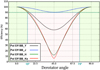 |
Fig. C.1. Measurements of the instrumental polarisation efficiency (not accounting the telescope) for four BB filters. For best use of the DPI mode, the pink zone where the efficiency drops below 90° (> 10° loss due to cross-talks) is avoided. For that, the derotator angle remains at < 15° or > 75° (from SPHERE User Manual). |
 |
Fig. C.2. Derotator position for NB observations, Cnt H, Cnt K1, and Cnt K2. The red bands indicate the zones to avoid when using BBs. |
A substantial fraction of our observations were conducted within the −15° →15° range, i.e. on optimal position for BB filters. However this is notably not the case for some images taken with the Cnt K1 and Cnt K2 filters. Contrary to Cnt K1, whose results look very compatible to what was observe in BBs, Cnt K2 maps, when created without selection (first panel of Figs. C.3–C.5), show low polarimetric signals. These maps also do not exhibit a realistic polarisation position angle (first panel of Fig. C.5), as discussed in Sect. 3.4. We therefore investigated the possible relation between this lack of signal and the derotator position and thus compared the final maps computed with all raw images, and those obtained with a selection of raw images with an optimised derotator position. All final images are shown in Figs. C.3–C.5 and reveal that selection does significantly affect the measured polarisation because the south-western arcs display very different polarisation (flux and degree).
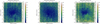 |
Fig. C.3. Binned maps of linear degree of polarisation (in %) in NGC 1068 with Cnt K2. These maps were created using all available raw images for first panel, only the 60% of the frames outside the 15−75° red zone of Fig. C.2 (last two series of points) for second panel, and only the first series of points (40%) within the red zone for the third panel. Third panel: binned version of maps shown in Fig. 4. |
As revealed by Figs. C.3–C.5, the derotator position angle affects the measured polarisation degree and position angle, but also when outside the 15−75° angle range, for Cnt K2. Maps created using data taken with angles > 75° show very low levels of polarisation. For this reason, we selected the first 40% of the frames within the 15−75° region, but with lower instrumental depolarisation for Cnt K2 data reduction (Fig. 4).
Even though we had a higher polarimetric signal, for the same reasons we also conducted the same experiment on Cnt K1 filter. Selection processes do not display such differences between final products and we thus keep the complete set of data for the data reduction for this NB.
Appendix D: The case of Cnt K2
It is already known (see e.g., the SPHERE user manual) that the SPHERE derotator position has an impact on the measured polarisation, at least in the BBs. This has been studied and depicted in the SPHERE instrument documentation. However, investigations by the SPHERE team have been conducted only on the BB filters, while the NB filters, including Cnt K2, have not been characterised yet. Therefore, we cannot derive strong conclusions about the exact impact of the depolarisation on the images in the NB filters. As the NB measurements in Cnt H and Cnt K1 filters are rather consistent with BB measurements, we are however more confident in the derived parameters, while Cnt K2 output should be considered carefully, especially the polarisation position angle. An analysis of the derotator positions in our data sets is detailed in Appendix C and shows a clear variation of the polarisation as a function of the derotator for Cnt K2; no clear evidence was found for other bands. We thus selected, according to this study, the image set that introduced the lower possible depolarisation.
With this set, it is clear that polarised signal does exist in Cnt K2 band as shown by the polarised intensity map of Fig. 4 (upper right and lower left panels), harbouring the two south-western arcs. In order to better represent the polarimetric signal in the maps in this NB, we show in Fig. D.1 the polarimetric maps using the binned I, Q, and U maps. The south-western arcs are clearly identified on the polarisation degree map; binning reduces the effect of the noise onto the polarimetric signal by averaging the intensity of a group of pixels. However, this binning does not seem to improve significantly the polarisation position angle map.
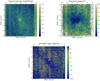 |
Fig. D.1. Binned 8 × 8 maps of NGC 1068 in Cnt K2. These maps show the binned version of the Cnt K2 maps of Fig. 4 for polarised intensity (in log10(ADU/s), first row, left panel) with polarisation vectors over-plotted, linear degree of polarisation (in %, first row, right panel), and linear angle of polarisation (in degrees, second row). |
All Tables
Contribution of dichroism to the polarised flux in different apertures for a given band (in %).
All Figures
|
Fig. 1. Maps of intensity (in log10(ADU/s), upper left panel), polarised intensity (in log10(ADU/s), upper right panel), linear degree of polarisation (in %, lower left panel), and linear angle of polarisation (in degrees, lower right panel) in NR (645.9 nm) with ZIMPOL. North is up and east is to the left. |
| In the text | |
|
Fig. 2. Maps of intensity (in log10(ADU/s), upper left panel), polarised intensity (in log10(ADU/s), upper right panel), linear degree of polarisation (in %, lower left panel), and linear angle of polarisation (in degrees, lower right panel) in Cnt H (1573 nm). Polarisation vectors have been over-plotted to the polarised intensity maps of upper right panel, with a length relative to the local polarisation degree. A reference length for a 5% vector is shown. North is up and east is to the left. |
| In the text | |
|
Fig. 3. Same as Fig. 2 for Cnt K1 (2091 nm). The red arrows indicate the position of the two south-western arcs. |
| In the text | |
|
Fig. 4. Same as Fig. 2 for Cnt K2 (2266 nm). The red arrows indicate the position of the two south-western arcs. |
| In the text | |
|
Fig. 5. Position of the apertures along the two arcs, south-west from the central source, on top of a polarisation degree map in H (1.6 μm). |
| In the text | |
|
Fig. 6. Degree (in %, first row) and angle (in degrees, second row) of polarisation as a function of position in the arc, from east to west, for the inner south-western arc (first column) and the outer south-western arc (second column), for all the observing bands (colour coded). Average value of the polarisation degree in a given band is indicated by the respective colour horizontal lines. Second row: the blue line corresponds to the expected polarisation position angle for these apertures if due to single scattering of light coming from the photo-centre of the AGN. |
| In the text | |
|
Fig. 7. Degree of polarisation (in %), averaged for all 8 apertures in both arcs (colour coded) as a function of wavelength. |
| In the text | |
|
Fig. 8. Position and size of the apertures used for polarimetric measurements, superimposed to the differential polarisation angle map of BB H (1625 nm, from Gratadour et al. 2015). The orange aperture corresponds to the very centre, the green to the off-centre, and the red to the central region as described in text. |
| In the text | |
|
Fig. 9. Degree (in %, left panel) and angle (in degrees, right panel) of polarisation as a function of wavelength (in nm) for the three apertures in the central region of NGC 1068. Very centre refers to the very inner 0.2″, off-centre to the region with an offset on the torus extension direction, and central region to the large aperture integrating all the flux. See text of Sect. 3.3 for more details about these apertures. |
| In the text | |
|
Fig. 10. Spectra of polarised intensity (first panel, with arbitrary intensity unit) and degree of polarisation (second panel) from dichroism simulated with MontAGN. |
| In the text | |
|
Fig. 11. Spectra of relative polarised intensity (first panel) and normalised polarisation Q intensity (second panel) for an AGN emission from MontAGN simulations. Polarised intensity is normalised to the maximum of the dichroic flux. |
| In the text | |
|
Fig. 12. Spectra of relative intensity (first column) and degree of polarisation (second column) for an AGN with dilution fractions of 50% (first row) and 80% (second row) from MontAGN simulations. Intensity is normalised to the maximum of the dichroic flux as detailed in text. |
| In the text | |
|
Fig. 13. Least-squares maps (in log scale) for r1:1.5 (left panel) and r1:2 (right panel) for dilution fraction varying between 0% and 100% (horizontal axis) and for optical depth τV between 2.5 and 200 (vertical axis). |
| In the text | |
|
Fig. 14. Degree of polarisation (in %) as a function of wavelength (in nm) for both simulations and observations. The measurements are the same as in the first panel of Fig. 9 and represent the very centre in orange, the off-centre region in green, and the whole central region in red. The simulated spectra are shown in a continuous blue line for a grain ratio of 1:1.5 and dashed line for a ratio of 1:2, with corresponding optical depth and dilution fraction parameters to best fit the very-centre (orange) data points. |
| In the text | |
|
Fig. 15. Simulated map of polarisation degree (left) and polarisation position angle (right) computed by MontAGN for an integrated optical depth of τV = 45 along the equatorial LOS, with an inclination angle of 90° at 1.6 μm (without dichroism and without dilution). |
| In the text | |
|
Fig. 16. Zoom on the polar extension of the detected polarisation degree, close to the very centre, on the Cnt K1 map (2.1 μm). Size of the image is ≈1.5 × 2″ and colour scale is the same as Fig. 3. |
| In the text | |
|
Fig. C.1. Measurements of the instrumental polarisation efficiency (not accounting the telescope) for four BB filters. For best use of the DPI mode, the pink zone where the efficiency drops below 90° (> 10° loss due to cross-talks) is avoided. For that, the derotator angle remains at < 15° or > 75° (from SPHERE User Manual). |
| In the text | |
|
Fig. C.2. Derotator position for NB observations, Cnt H, Cnt K1, and Cnt K2. The red bands indicate the zones to avoid when using BBs. |
| In the text | |
|
Fig. C.3. Binned maps of linear degree of polarisation (in %) in NGC 1068 with Cnt K2. These maps were created using all available raw images for first panel, only the 60% of the frames outside the 15−75° red zone of Fig. C.2 (last two series of points) for second panel, and only the first series of points (40%) within the red zone for the third panel. Third panel: binned version of maps shown in Fig. 4. |
| In the text | |
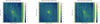 |
Fig. C.4. Same as Fig. C.3 but for the linearly polarised flux (in ADU/s). |
| In the text | |
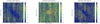 |
Fig. C.5. Same as Fig. C.3 but for the linear polarisation position angle (in degrees). |
| In the text | |
|
Fig. D.1. Binned 8 × 8 maps of NGC 1068 in Cnt K2. These maps show the binned version of the Cnt K2 maps of Fig. 4 for polarised intensity (in log10(ADU/s), first row, left panel) with polarisation vectors over-plotted, linear degree of polarisation (in %, first row, right panel), and linear angle of polarisation (in degrees, second row). |
| In the text | |
Current usage metrics show cumulative count of Article Views (full-text article views including HTML views, PDF and ePub downloads, according to the available data) and Abstracts Views on Vision4Press platform.
Data correspond to usage on the plateform after 2015. The current usage metrics is available 48-96 hours after online publication and is updated daily on week days.
Initial download of the metrics may take a while.