| Issue |
A&A
Volume 652, August 2021
|
|
|---|---|---|
| Article Number | A65 | |
| Number of page(s) | 19 | |
| Section | Extragalactic astronomy | |
| DOI | https://doi.org/10.1051/0004-6361/202141349 | |
| Published online | 11 August 2021 | |
The inner hot dust in the torus of NGC 1068
A 3D radiative model constrained with GRAVITY/VLTi
1
LESIA, Observatoire de Paris, Université PSL, CNRS, Sorbonne Université, Université de Paris, 5 Place Jules Janssen, 92195 Meudon, France
e-mail: This email address is being protected from spambots. You need JavaScript enabled to view it.
, This email address is being protected from spambots. You need JavaScript enabled to view it.
2
Kavli Institute for Particle Astrophysics & Cosmology (KIPAC), Stanford University, Stanford, CA 94305, USA
Received:
19
May
2021
Accepted:
4
June
2021
Abstract
Context. The central region of NGC 1068 is one of the closest and most studied active galactic nuclei. It is known to be type 2, meaning that its accretion disk is obscured by a large amount of dust and gas. The main properties of the obscuring structure are still to be determined.
Aims. We aim to model the inner edge of this structure, where the hot dust responsible for the near-infrared emission reaches its sublimation temperature.
Methods. We used several methods to interpret the K-band interferometric observables from a GRAVITY/VLTI observation of the object. At first, we used simple geometrical models in image reconstructions to determine the main 2D geometrical properties of the source. In a second step, we tried to reproduce the observables with K-band images produced by 3D radiative transfer simulations of a heated dusty disk. We explore various parameters to find an optimal solution and a model consistent with all the observables.
Results. The three methods are consistent in their description of the image of the source, an elongated structure with ∼4 × 6 mas dimensions and its major axis along the northwest–southeast direction. The results from all three methods suggest that the object resembles an elongated ring rather than an elongated thin disk, with the northeast edge appearing less luminous than the southwest one. The best 3D model is a thick disk with an inner radius r = 0.21−0.03+0.02 pc and a half-opening angle α1/2 = 21 ± 8° observed with an inclination i = 44−610° and PA = 150−138°. A high density of dust n = 5−2.5+5 M⊙ pc−3 is required to explain the contrast between the two edges by self-absorption from the closer one. The overall structure is itself obscured by a large foreground obscuration AV ∼ 75.
Conclusions. The hot dust is not responsible for the obscuration of the central engine. The geometry and the orientation of the structure are different from those of the previously observed maser and molecular disks. We conclude that a single disk is unable to account for these differences, and favor a description of the source where multiple rings originating from different clouds are entangled around the central mass.
Key words: galaxies: active / galaxies: nuclei / galaxies: Seyfert / radiative transfer / infrared: general
© P. Vermot et al. 2021
 Open Access article, published by EDP Sciences, under the terms of the Creative Commons Attribution License (https://creativecommons.org/licenses/by/4.0), which permits unrestricted use, distribution, and reproduction in any medium, provided the original work is properly cited.
1. Introduction
In this paper, we present a study of the active galactic nucleus (AGN) of NGC 1068, one of the closest AGNs to the Milky Way. Located at a distance of 14.4 Mpc (Bland-Hawthorn et al. 1997), the spatial scale is 70 pc/″ (these conventions are maintained throughout the paper). This proximity, coupled with other observational advantages such as a high luminosity and the absence of foreground emission or absorption, make NGC 1068 a key target in the observation of AGNs, and have led to a wealth of publications. The observation of its polarised spectrum led authors to postulate the presence of a dusty torus, and more globally to the unified model of AGNs proposed by (Antonucci & Miller 1985; Antonucci 1993).
The NGC 1068 nucleus is a complex region where many structures and various physical conditions coexist. From large to small scales, the main components of interest for this study are as follows. The extended region of ionized gas –the narrow line region (NLR)– can be considered as the largest structure of the AGN. It has a characteristic bicone or hourglass shape oriented northeast–southwest and a motion interpreted as an outflow ejected from the nucleus (Das et al. 2006; Poncelet et al. 2008; Gratadour et al. 2015). The north pole is oriented towards the observer, with i = 5° −10° and PA ∼ 30°. Two ionization mechanisms are invoked to explain the emission line properties: photoionization from the accretion disk UV-X radiation (Kraemer & Crenshaw 2000; Hashimoto et al. 2011; Vermot et al. 2019) and ionization from shocks due to the interaction between the jet and the interstellar medium (Dopita & Sutherland 1996; Exposito et al. 2011).
The most external regions of the torus are cold and not luminous. However, using polarimetric imaging techniques, Gratadour et al. (2015) detected an elongated 60 × 20 pc structure oriented with PA = 118° tracing scattering of the photons, which is interpreted as the signature of the torus. Another structure, highly polarized, is detected. Its orientation largely differs from the first, with PA = 56°. Referred to as the “ridge” by the authors, it could arise from dichroic absorption by the dust (Grosset et al. 2018, 2021; Grosset 2019).
At smaller spatial scales, thanks to ALMA observations, Gallimore et al. (2016), García-Burillo et al. (2016, 2019) highlighted a disk of molecular gas, an elongated 10 × 7 pc structure, orientated with PA = 112° and Mgas = (1 ± 0.3)×105 M⊙, with a complex geometry and dynamics. Indeed, in addition to the enhanced turbulence, it has been shown that this disk is counter-rotating (Impellizzeri et al. 2019; Imanishi et al. 2020) when compared to the inner region where maser spots are detected (Greenhill et al. 1996; Greenhill & Gwinn 1997; Gallimore et al. 2001).
At similar scales, information on the warm dust has been gathered using the VLTI/MIDI instrument, leading to many published studies (Jaffe et al. 2004; Weigelt et al. 2004; Poncelet et al. 2006; Raban et al. 2009; Burtscher et al. 2013; López-Gonzaga et al. 2014). These studies agree in their description of the central source as a 1.4 pc × 0.5 pc elongated structure with PA ∼ 130° −135°. The temperature of the dust is estimated to be between 600 K and 800 K. These studies also revealed the presence of a polar emission from colder dust (T ∼ 300 K) –providing a significant contribution to the flux– which could originate from the inner edge of the ionization cone (Raban et al. 2009).
Very Long Baseline Array (VLBA) observations revealed even smaller structures, both through continuum (Gallimore et al. 1996, 2001, 2004) and maser emission (Greenhill et al. 1996; Greenhill & Gwinn 1997; Gallimore et al. 2001). The source of continuum emission, named S1 at these wavelengths, is resolved with an elongated shape of 0.4 × 0.8 pc and a major axis oriented along PA ∼ 110°. A detailed analysis of its spectrum by Gallimore et al. (2004) concluded that it results from free-free emission by gas heated to high temperatures by the central UV-X source. This led to a lower limit on its luminosity: LUV-X ≥ 7 × 1037 W. The detection of H2O maser spots provides a very reliable and precise measurement of the emitting medium. A line of maser spots oriented along PA = 135° is observed as far as 1.1 pc from the nucleus. The analysis of their velocity profile indicates that they originate from a disk seen edge-on with an inner radius ri = 0.6 pc and an outer radius ro = 1.1 pc. This maser disk is counter-rotating with the molecular disk observed with ALMA. The maser disk appears to be contained within the molecular disk and surrounds the cloud of gas from which S1 originates.
A study based on similar GRAVITY data was presented by GRAVITY Collaboration (2020), who focus on the interpretation of a reconstructed image of the source and suggest that the K-band emission originates from a thin ring-like structure with a radius r = 0.24 ± 0.3 pc, PA = 130 ±°, and inclination i = 70° with the north pole pointing toward the observer. Below, we present a new analysis of this observation, focusing on the modeling of a subset of data with radiative transfer simulations.
2. Observation
The GRAVITY observation on which this study is based was made during the night of November 20, 2018, under excellent atmospheric conditions. It is one of the two observations used in GRAVITY Collaboration (2020).
However, NGC 1068 remains a challenging target to observe with GRAVITY because of its relatively low surface brightness and complex morphology. In order to achieve the observation, 100% of the flux from the source was injected in the fringe-tracker (FT; see GRAVITY Collaboration 2020). This strategy made it possible to fringe track, although this means that only FT data are available, with a R ∼ 22 spectral resolution (K-band split into five spectral channels) and without any absolute phase measurements.
The total integration time on the object is 45 min, and three reference stars have been observed, HIP 54, HIP 16739, and HIP 17272. Data reduction was done with the standard pipeline provided by ESO. Among others, this procedure provides squared visibility and closure phase measurements.
3. Data and interferometric observables
3.1. u–v plane
The spatial frequencies at which the interferometric observables are sampled form the u − v plane of the observation, and are represented in Fig. 1. The sampled spatial frequencies range from 15 × 106 λ to 60 × 106 λ, which probes spatial scales ranging from 3 to 12 mas. The northeast–southwest direction (red, purple, and green bases on Fig. 1) is much more densely sampled than the orthogonal northwest–southeast direction (blue base).
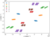 |
Fig. 1. u − v plane associated to the UT observation. (0) UT3–UT4, (1) UT2–UT4, (2) UT1–UT4, (3) UT2–UT3, (4) UT1–UT3, (5) UT1–UT2. |
3.2. Visibility
For each point of the u − v plane, two visibility estimators are provided by the pipeline, namely the visibility amplitudeVamp and the squared visibilityV2. Here we use this second estimator, which is less sensitive to phase variations and consequently to atmospheric turbulence. Hereafter, the square root of squared visibility will simply be referred to as the visibility. Data were selected by removing the visibility points associated with the shortest spectral channel. Their measurement is known to be degraded by the presence of the GRAVITY metrology laser operating at these wavelengths, as is confirmed by the corresponding inconsistent visibility values.
The visibility points are presented in Fig. 2, and are color-coded according to the baseline. We first notice a drop in the visibility with increasing spatial frequency up to 25 Mλ where it reaches zero before slightly increasing at larger frequencies. This indicates that the source is spatially resolved by the interferometer and has a size of between 5 and 20 mas. The ‘rebound’ of the visibility at large frequencies indicates that the main structure exhibits sharp edges. Secondly, the visibility values well below 1 ( ) reveal that a significant part of the flux comes from a source that can be considered diffuse with respect to the resolution and field of view of GRAVITY with the Unit Telescopes (UT). Figure 3 represents the same visibility points but color-coded according to wavelength. The visibility can be seen to increase with wavelength, indicating either that the morphology of the object significantly differs from one wavelength to another, or that the ratio of the coherent flux to the total flux increases with wavelength.
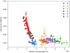 |
Fig. 2. Squared visibility color-coded according to baseline : (0) UT3–UT4, (1) UT2–UT4, (2) UT1–UT4, (3) UT2–UT3, (4) UT1–UT3, (5) UT1–UT2. |
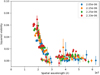 |
Fig. 3. Squared visibility color-coded according to wavelength (in meters), as listed in the legend. |
The pipeline provides an estimation of the uncertainty associated with the visibility measurement. A detailed study of these estimates revealed that they may not be representative of the actual error on the measurements. Indeed, a significant number of them have ΔV2 < 5 × 10⁻⁴, well below the scattering of data points observed at the same wavelength and very close spatial frequency. We estimate that this may come from the presence of systematic uncertainties, which are usually not significant compared to the statistical uncertainties but could become significant in this case. Indeed, the faintness of the source might lead to high systematic uncertainties due to fluctuating AO correction, fiber injection, or fringe jumps. To take into account these systematic errors, we measured the scattering of carefully chosen points at similar wavelength and spatial frequency and decided to add a constant ΔV0 = 0.0015 uncertainty to every visibility measurement. This allows us to overcoming problems that occurred with points associated to a very low uncertainty that took an unreasonable importance in the χ2 fitting procedures, while still taking into account the statistical uncertainties (which for some points can be significant).
3.3. Closure phase
The closure phase measurements are presented in Fig. 4 and Table 1 summarizes some statistical properties of the triplet measurements.
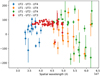 |
Fig. 4. Closure phase color-coded per triplet. |
Basic statistical properties of the closure phase measurements.
Two remarks can be made from this first statistical analysis. First, of 104 closure phase measurements, 60 are provided by the [UT1–UT2–UT3] triplet. Moreover, the uncertainties estimated on the points coming from this triplet are much smaller than those from the three others: the median of the uncertainties is 3° for [UT1–UT2–UT3] while it is 21° for the 44 other measurements. As a consequence, in the analysis below, this triplet has a larger weight in the data fitting involving the closure phase measurements. Second, the closure phase mean value for this triplet differs from zero ( ), which already indicates that a significant asymmetry is present in the source luminosity distribution.
3.4. Coherent spectrum and magnitude
The coherent flux measurements provided by GRAVITY present a very large scatter, most probably due to the efficiency in the fiber injection which varies during the observation. Hence, this observation cannot be used alone, and we computed the mean of this observable over all spatial frequencies instead in order to obtain an estimation of the spectrum of the resolved source. Hereafter, we refer to this spectrum as the coherent spectrum; it is the the four-point low-resolution spectrum (R ∼ 22) in arbitrary units presented in Fig. 5. We notice that the flux increases with wavelength, and that a slight excess is present at 2.15 μm. Considering the uncertainties associated to this spectrum, this could be due to random fluctuation. However, we note that this could also indicate the presence of a strong Brackett γ emission line.
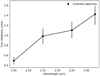 |
Fig. 5. Observed coherent spectrum. |
Finally, the detailed analysis of the images from the acquisition camera presented in GRAVITY Collaboration (2020) provides an estimation of the total K-band magnitude injected in the fiber: Ktot = 8.33 ± 0.25.
3.5. Auxiliary telescope observation
We decided not to include in our analysis another observation that was performed with the auxiliary telescopes (ATs) of the VLTI. The motivation for this decision is twofold. First, it is difficult to merge the visibility measurements from the UT and AT observations. Indeed, at least two incompatibilities appear in the visibility measurements made on adjacent and over-imposed baselines from the two observations. We consider that these differences appear because of the different relative contributions of the diffuse background to the AT and UT fields of view. Indeed, the fibers of the UT have a ∼60 mas field of view (FoV) while those of the AT have a 240 mas FoV. In the following sections, as already stated in GRAVITY Collaboration (2020) and as suggested by the MIDI observations, we show that the diffuse background contributes significantly to the total flux injected in the UT FoV. As a consequence, the diffuse flux in the FoV of the AT is likely larger than the UT, while the flux from the resolved structure will remain identical. In that case, if these effects are not included in the model, these jumps in the visibility measurement might be incorrectly interpreted as resulting from a feature of the resolved source.
A model of these extended structures would be required to take into account their respective effect on each FoV. This is especially true because this effect appears to vary according to the direction of the baseline. In the upcoming analysis, we assume that the diffuse contribution is uniform. While it might be sufficient for the very small scales that we are modeling, such an assumption cannot be valid at the spatial scale of the AT FoV. The second motivation to discard the AT observations was to focus on the smaller spatial scales probed with the UT.
4. Modeling
4.1. Geometrical approach
As a first step, we used geometrical approaches to model the observables and derive images of the source: we used simple geometrical models fitted with the LITpro software1 as well as image reconstructions using the software MiRa (Thiébaut et al. 2003). The goal was to look for characteristic size measurements and hints about the morphology to guide our further radiative transfer modeling.
All simple geometrical models converge toward a central elongated structure (see Table 2), with ∼4 × 6 mas (∼0.28 × 0.42 pc) dimensions and a major axis at PA ∼ 140°. Also, all models agree on the significance of the diffuse flux, namely that it contributes around two-thirds of the total flux. Of the four simple models presented in Table 2, the one that provides the best fit to the data is the elongated thick ring, whose K-band image and associated visibility points are presented in Fig. 6.
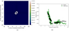 |
Fig. 6. a: image in arbitrary flux units of the best geometrical model, an elongated thick ring over-imposed on diffuse emission. b: comparison between the observed and the modeled visibilities. |
Results of the fit performed for each geometrical model.
As in GRAVITY Collaboration (2020), from our simple image reconstruction attempts we conclude on the presence of an inclined ring or disk with a radius of ∼3.5 mas (0.25 pc), an elongation ratio of L/l ∼ 0.5, and a less luminous northeast edge. Still, we observe significant variations in the aspect of the source from one reconstruction to another, especially along the poorly sampled northwest–southeast direction, which prevent us from reliably constraining a model based on the images.
We also note that this first modeling is consistent with results from VINCI (Wittkowski et al. 2004) and the MIDI observation (Jaffe et al. 2004; Hönig et al. 2008; Raban et al. 2009; López-Gonzaga et al. 2014) which revealed a structure with a very similar orientation. However, these latter studies found a larger size for the structure, which can be explained by the differences in temperature probed by the two instruments.
4.2. Physical modeling from radiative transfer simulations MontAGN
In this section, we describe how we used radiative transfer simulations to derive a physically realistic 3D model of the source from the GRAVITY observables. Here we tried a new approach, using a model that is highly constrained from astrophysical considerations in order to produce physically realistic images, which we compared to the interferometric measurements in a second step. For this purpose, we used the simulation code MontAGN (Grosset et al. 2018; Grosset 2019) to model a dusty disk heated by a central source of energetic photons. The images produced by each model were used to compute the various interferometric observables.
We first give a description of MontAGN, and general considerations on the model used. We then describe two sets of simulations: the sole purpose of the first one is to reproduce the visibility and the photometric measurements, while the second one is specially designed to additionally take into account the closure phase measurements.
4.2.1. MontAGN
MontAGN is a radiative transfer simulation code using Monte Carlo methods, developed to study AGN dusty tori, and more specifically to interpret polarimetric observations. It offers the possibility to model the diffusion, absorption, and emission of photons by dusty structures with arbitrary geometries for a wide range of dust types.
MontAGN follows the path of photons, from their emission by a central source until the moment they exit the simulation grid, modeling the different interactions that take place with the medium along the way. In the following list, we succinctly describe the main steps of interest of a simulation:
1. Extinction and absorption coefficients, albedo, Mueller matrices, and phase functions are calculated on a wide range of wavelengths (from X to far-IR) and grain sizes for each of the “dust types” defined by the user.
2. The 3D grid of cell is initialized with Cartesian coordinates, and is filled with dust by attributing a density value for each cell and each dust type.
3. Photons are emitted by the central source with a random direction, by monochromatic packets, with an initial wavelength that is randomly chosen according to the source spectral energy distribution (SED).
4. Each packet of photons propagates freely in a straight line through empty cells. When the packet enters a cell that is not empty, densities are used to randomly decide whether or not the photon will interact with the cell. If it does not, it pursues its straight line propagation.
5. If the photon interacts with the cell, the type and size of the grain with which it will interact, then the type of interaction (absorption or diffusion), are randomly chosen according to the densities, extinction coefficients, and albedo of the different grains present in the cell.
6. If the photon is scattered, its wavelength remains unchanged, its new direction is chosen from the phase function of the selected grain, and its Stokes vector is updated. If the photon is absorbed, the temperature of the cell is updated, and a new packet of photons with the same energy is emitted in a new direction, with a wavelength that is randomly chosen to match the Planck emission of the cell.
7. Eventually the photons exit the simulation grid. Their properties are then stored in an output file.
8. From these files, which contain information on every photon exiting the simulation grid, images can be generated for any position of the observer and any spectral domain.
4.2.2. Base model
We model the hot dust of the inner region of the dusty torus of NGC 1068 with graphite grains distributed up to the sublimation limit in a thick disk-like structure (see Fig. 7) with a uniform density. Guided by the size estimations from geometrical models and image reconstructions, the grid has been chosen to be contained in a 1 × 1 × 1 pc cube with 0.025 pc cells.
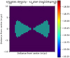 |
Fig. 7. Geometry of the thick disk model used in the MontAGN simulations. The image is a cut along any direction orthogonal to the equatorial plane of the structure. |
Interstellar dust mostly contains two grain types, namely graphite and silicate (Barvainis 1987; Netzer 2015), which are simultaneously present in most astrophysical conditions. However, close to the accretion disk of an AGN, dust grains are heated by the UV-X emission until they sublimate. Two distinct arguments point to the conclusion that silicate grains will reach sublimation at a larger distance from the accretion disk than graphite grains, which would then be the sole grain type populating this inner region of the dusty tori: First, silicate grains dispel their thermal energy in the infrared less efficiently than graphite grains, while they absorb UV-X photons similarly. Therefore, at a given distance from the central source, silicate grains will be found at higher temperatures. Second, the sublimation temperature of silicate grains is lower than that of graphite grains (Barvainis 1987; Baskin & Laor 2018, Tsub, silicates ∼ 1400 K, Tsub, graphites ∼ 1700 K). Hence, our model only contains graphite grains and we hypothesize that the inner radius of the dusty structure coincides with the distance at which they sublimate. The size distribution of the grains (n grains of size a) is assumed to follow a MRN power-law (Mathis et al. 1977) with dn/da ∝ a−3.5 and amin = 5 nm and amax = 250 nm. Given this size distribution, the mean density of grains specified as an input of the model, and the geometry of the structure, we can compute the total mass of dust of the model.
To describe the geometry of the hot dust structure, we use a simple model, with a geometrically thick disk defined by its inner radius, outer radius, and opening angle (see Fig. 7). As we see in the following section with the images generated by MontAGN, the luminosity of the dust decreases very quickly with the distance to the central source and most of the K-band emission comes from a region very close to the sublimation distance, forming a thick ring. Hence, the large-scale structure of the torus has little impact on the image of the object at these wavelengths and a more complex model is not required at this stage. The opening angle of the structure (i.e., the thickness of the disk) will be a variable parameter, as will its inner radius. The outer limit is defined by the grid limits.
At last, because the accretion disk of NGC 1068 is obscured and little information is known about its actual spectrum, to describe the central source (considered as point-like) we use a simple spectrum similar to the one used in Hönig et al. (2006) (see Fig. 8). Also, it emits the vast majority of its flux in the UV-X domain, with a negligible infrared luminosity. We note that for verification, we ran a few simulations with other central spectra, without any detectable effect as long as most of the energy is emitted in the UV-X domain. For a given type of grain and a given central source spectrum, the sublimation radius is only determined by the luminosity of the source.
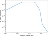 |
Fig. 8. Spectrum of the central source used in MontAGN simulations. |
4.2.3. MontAGN model 1: accounting for visibilities, photometry, and spectral variations
For the first model, to constrain the geometry of the source and the main scaling parameters of the model, we only focus on reproducing the visibility points without taking into account the closure phase. More precisely, we explore the values of the sublimation radius, the opening angle, the inclination, and polar angle (PA) parameters as reported in Table 3.
MontAGN simulation parameters for model 1.
Once a simulation with a given sublimation radius and opening angle is finished, K-band images with a 2.5 pc × 2.5 pc FoV and 0.025 pc pixel size are generated for a range of inclinations. The discrete Fourier transforms are computed and linearly interpolated at the spatial frequencies observed with GRAVITY. Polar angle (PA) values are explored by a change of coordinates so that fewer images have to be computed.
The spectrum of the model never matches the observed coherent spectrum: it is more blue in comparison, even in the most favorable cases. Moreover, the analysis of the simulation reveals that the models are too luminous when compared to the K-band magnitude. These two remarks suggest that the infrared emission of this region is significantly absorbed by foreground material. To match the observed K-band magnitude, we fit for each set of parameters a standard extinction (Cardelli et al. 1989) by applying its effect uniformly on the initial MontAGN images. The AV values reported in Tables 4 and 6 correspond to this extinction, which is not caused by the hot dusty structure, but rather by foreground colder material. We then deduce the spectrum of the diffuse component required to match the observed visibility.
Best-fit parameters from model 1.
Table 4 gives the value of the best-fit parameters and Fig. A.1 shows cuts around this best solution in the 4D χ2 cube. The inner radius, the inclination, and the position are well constrained, with well-defined minima. However, two solutions are possible for PA, separated by exactly 180°, which highlights the limitations of a modeling performed solely on visibility measurements. The opening angle of the disk is not well constrained, and even if an optimal solution is obtained, the χ2 analysis reveals that we can only reliably consider an upper limit on this parameter: α1/2 ≤ 25°.
From Fig. A.1, we also notice that one slight degeneracy seems to appear between the inclination and the sublimation radius. This is explained by the fact that given the u − v plane of the observation, the information contained in the visibility is mostly a measurement of the spatial extent of the structure in the northeast–southwest direction.
Figure A.3 shows the K-band image associated to this best solution. Because of the  inclination, the source appears as an inclined ring. The low density of dust used in this model explains both the symmetric aspect of the structure and the fact that the northwest and southeast extremities are more luminous, because they correspond to lines of sight that are geometrically crossing more hot dust.
These results are in good agreement with the ones from the geometric models presented in Sect. 4.1 and in GRAVITY Collaboration (2020), indicating that the K-band emitting structure resembles an inclined ring with PA ∼ 135°.
4.2.4. MontAGN model 2: accounting also for the closure phase
In a third model, we try to reproduce the GRAVITY closure phase and visibility measurements simultaneously. As already pointed out in Sect. 3.3, the [UT1–UT2–UT3] triplet (in red in Fig. 4) contains the majority of the closure phase measurements and is moreover associated with the lowest uncertainties. The spatial frequencies probed by this triplet allow us to constrain an important property of the model: the difference in luminosity between the northeast and the southwest regions of the structure. The closure phase is positive when the southwest edge is the most luminous, and negative if the northeast edge is the most luminous. The value of these closure phases is an indicator of the relative contrast between the two edges. The mean closure phase on the [UT1–UT2–UT3] triplet is 73°, which implies a high contrast.
The first dataset of MontAGN simulations, which was used for model 1 in Sect. 4.2.4, produces very symmetric images which do not allow us to reproduce this contrast and the closure phase measurements. However, increasing the dust density of the disk in MontAGN simulations results in an increase in the contrast between the two edges: the closest edge becomes optically thick, self-absorbs the infrared photons it emits, and as a result, its K-band luminosity is decreased. Hence, the value of the closure phase of the resulting model for the [UT1–UT2–UT3] triplet gets closer to those observed.
In order to investigate this new aspect of the model, we performed new simulations with a coarser sampling for the opening angle (accounting for the difficulty in constraining this parameter and to save time) and with a wide range of dust densities (testing up to 40 grains per cm3 was necessary to converge toward a solution). Table 5 summarizes the parameters used for the model. The comparison with the visibility measurements is similar to the one performed for model 1. As the complex discrete Fourier transform of the images has already been computed and interpolated at the spatial frequency probed by the baselines, the computation of the closure phase is direct. The presence of a diffuse background, a foreground extinction, and the luminosity of the source does not influence these closure phase measurements, so there is no additional correction to apply.
MontAGN simulation parameters for model 2.
We computed two 5D χ2 maps, one for the visibility predictions of the model and one for the closure phase. After normalization, which was performed so that the minimum of each hypercube is equal to the number of data points of the associated observable, these maps were added to get the final χ2 estimator.
The various 2D χ2 maps are presented in Fig. A.5. It is interesting to note that there is a slight degeneracy between the opening angle and the inclination, maintaining the annular aspect of the source. Nevertheless, these maps highlight the existence of a well-defined and unique solution in the explored parameter space. The best model parameters are presented in Table 6. Some properties from previous models are maintained, but, in addition to providing a constraint on the dust density, the inclusion of the closure phase impacted some of the geometrical parameters.
Best-fit parameters for model 2.
A comparison between the observed and the predicted visibility is presented in Fig. 9, and a comparison of the closure phase is shown in Fig. 10. The prediction of the visibility is similar to that obtained with model 1; the low spatial frequencies are well reproduced with their spatial variability, as is the rebound at high frequencies, even if the spectral dispersion is underestimated by the model at these frequencies. Except the shortest wavelength of the shortest baseline, this model reproduces the observed visibility and its spectral dependency well.
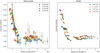 |
Fig. 9. Comparison between the observed visibility (left) and the one predicted by the MontAGN model 2 (right). |
 |
Fig. 10. Comparison between the observed closure phase (left) and the one predicted by the MontAGN model 2 (right). |
The predictions of the model closely agree with the observed closure phase measurements, particularly those related to the [UT1–UT2–UT3] triplet (blue), which carries most of the information. The [UT2–UT3–UT4] triplet (red) is also fairly well reproduced by the model, as is the [UT1–UT3–UT4] triplet (green) considering the uncertainties. However, the [UT1–UT2–UT4] triplet (orange), which probes the highest spatial frequencies, is not well reproduced by the model. The uncertainties on the values of this triplet and their scattering are high, which clearly indicates that this measurement lacks reliability. However, closure phase measurements are known to be very robust and we consider that a better explanation is that this observation traces an additional asymmetry at the smallest spatial scales, which cannot be reproduced by the models used in this work.
With i = 44° and α1/2 = 21°, the structure still resembles an inclined ring. However, its orientation is now estimated to be  , compared to ∼135 − 145° as suggested by previous models. Considering the estimated uncertainties, these values could be compatible, but the difference is significant. The closure phase provides an estimation of the density of the medium: ngrains = 10 cm−3. Finally, the temperature of the diffuse component is estimated to be T ∼ 600 K and the foreground extinction to be AV = 76.5 (i.e., AK = 8.9), very similar to the one deduced from the previous model.
The best K-band image of the source is presented in Fig. 11. It is compatible with our previous models in terms of shape and size, despite noticeable differences. The most significant such difference is the high contrast between the two edges of the structure. This can be explained as follows: for the southwest edge, we have a direct line of sight toward the surface of sublimation, while for the northeast edge it is obscured by the dust located in the line of sight, so that only the southern extremity of this edge can be observed. This last point may explain the finding that for a similar aspect of the image, this model corresponds to a lower inclination. Hence, knowing that the northeast edge is the least luminous allows us to state that the south pole of the structure is directed toward the observer.
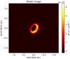 |
Fig. 11. K-band image of the MontAGN model 2. The diffuse background is not represented. |
The information presented in Fig. A.8 suggests that inside the dusty structure the temperature decreases very quickly with distance to the central source. This confirms that GRAVITY is observing only the most internal region of the torus, the inner rim. Figure 12 displays the spectra of the model for the compact source and for the diffuse background. The spectrum of the diffuse background is very well fitted by a T ∼ 600 K black-body emission, which is consistent with the large-scale structure temperature observed with MIDI in the mid-infrared (see Table B.1).
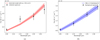 |
Fig. 12. Spectral fits for model 2. a: observed coherent spectrum and extincted model spectrum. b: diffuse background and temperature estimation. |
4.2.5. Unified model of the dataset
In the previous sections, we described several methods to interpret and model the GRAVITY data. Despite some diversity in the resulting parameters, recurrent features allow us to draw a synthetic description of the nuclear structures, which we present below before discussion and comparison with previous studies.
First, the flux of the compact object represents around one-third of the total flux detected in the field of view of GRAVITY (56 mas or 3.9 pc); the remainder is considered as a diffuse component distributed on larger spatial scales.
All the models agree on the characteristic size of this structure which is less than one parsec. More precisely, the different methods converge toward an elongated structure with a major axis of around 7 mas (0.5 pc) oriented northwest–southeast and with an elongation ratio of e ∼ 3/2.
The apparent image of the source is an elongated ring. This is suggested by the simple geometrical models, the image reconstructions, and the various MontAGN models. This aspect can be explained in three dimensions by a roughly toroidal structure observed from a latitude of between 35° and 45°.
The best model found to describe the infrared emission is an optically thick structure with a geometrically thick disk shape and composed of graphite heated by a central UV-X source. The inner radius of this disk, which coincides with the sublimation region of graphite, is between 0.20 pc and 0.25 pc, which corresponds to a central source of luminosity of between 3.9 × 1038 W and 6.4 × 1038 W. As we assume that the dust is at its sublimation temperature and that the central radiation is fully responsible of its heating, this value should be taken as an upper limit of the central UV-X luminosity. As this upper limit is relatively close to other independent estimations and lower limits (between a few 1037 and a few 1038 W according to Pier et al. 1994; Bland-Hawthorn et al. 1997; Kishimoto 1999; Gallimore et al. 2001), we confirm a posteriori that the dust must be close to its sublimation temperature and mostly heated by the central radiation.
The closer and further edges do not have the same luminosity, which can be explained by the self-absorption effect of secondary photons. It is possible to get an estimation of the density of the dust from this information, which in turn provides an estimation of the mass dust of the structure, Mdust ∼ 1.75 M⊙. Importantly, the whole region is obscured by a large quantity of interstellar dust located between the object and the observer. Reproducing the entirety of the observables, the MontAGN model 2 is considered the best model in the following and the following discussion refers to the parameters presented in Table 6 unless otherwise specified.
5. Discussion on the overall torus structure
The orientation of the hot dust structure that we deduce from the results of the present study seems incompatible with results from previous observations of the NGC 1068 nucleus. However, as further discussed below, the geometry and the dynamics of the torus at parsec scales is much more complex than what can be suggested by lower angular resolution observations. This observational complexity reveals an asymmetry, and possibly high turbulence or instabilities in the heart of the torus. From this perspective, two interpretations are discussed below to explain the observed discrepancies: a unique unstable disk, and an apparent superposition of entangled rings.
5.1. Discussion on the central structure inclination and orientation
Every method presented in this paper to model the GRAVITY data indicate an orientation of the structure in the range of 135° ≲PA ≲ 150° and an inclination of 40° ≲i ≲ 70°. The best model has  and
and  .
.
Nevertheless, several observations, as described below, suggest either an obscured nature of the nucleus, associated with an inclination of around 90°, which is well in line with the classical unified model of AGNs (Antonucci 1993), or a different orientation of the central structure from ours. First of all, the historical spectro-polarimetric observation of NGC 1068 (Antonucci & Miller 1985) revealed polarized Seyfert 1 emission in the heart of NGC 1068, interpreted as a type 1 nucleus hidden behind a large amount of dust (Antonucci 1993). This structure is assumed to be roughly toroidal –as is the case for our model– but seen close to edge-on for an obscured AGN such as NGC 1068. At first sight, our results seem to contradict this model.
The extended torus has been observed at the scale of a few tens of parsecs. Its very dimly lit outskirts were observed thanks to polarimetric techniques in Gratadour et al. (2015). The image of the object is elongated, with dimensions 60 pc × 20 pc, which suggests an edge-on structure. This signature of the extended torus is oriented with PA = 118° which differs by 15° to 30° from our estimations.
At subparsec scales, the VLBA radio continuum observations (Gallimore et al. 2004) also suggest the presence of an elongated structure, S1, which could trace an edge-on disk, with PA ∼ 110°. Moreover, the detection of many maser spots located on a line crossing the nucleus indicates without any ambiguity the presence of an edge-on disk, with i ∼ 90°. Nevertheless, this maser disk is not oriented with PA ∼ 110° as in the other structures mentioned so far, but with PA ∼ 135°, which is compatible with the lowest estimations obtained from GRAVITY data.
As we discuss below, the misalignment between these two radio structures (maser disk and S1) is also observed between structures at larger scales. To support this discussion, inclination measurements as well as position angles for the various observations are synthesized in Table B.1.
A structure with PA ∼ 145°. As in the previously mentioned maser orientation (Greenhill & Gwinn 1997), several observations have revealed the presence of one or more elongated structures oriented along PA ∼ 135° −140°. In particular, the 800 K dust observed with MIDI is oriented with 135 − 140°, exactly as the 1600 K hot dust observed with GRAVITY in this study. Also, López-Gonzaga et al. (2014) highlight a polar emission (located north of the central source) that is colder and more extended, with PA ∼ 145°. We also note that the highly polarized ridge observed in Gratadour et al. (2015) is approximately orthogonal to this PA ∼ 140° orientation, which could trace a polar counterpart.
Inclinations. Only a few observations provide an actual measurement of the inclination of the torus at parsec and subparsec scales. Indeed, i ∼ 90° found in the literature is more often a hypothesis motivated by the obscured nature of the nucleus or by the orientation of the NLR and jet rather than a direct measurement. As explained in Nixon & King (2013), the orientation of a jet originating from accretion around a black hole is very stable as it is linked to the rotation axis of the massive object. Its orientation is not expected to show any significant changes on timescales of τ ≤ 107 years, even in the case of chaotic accretion. In comparison, the timescale of a cloud orbiting at 0.5 pc from the central mass is τ ∼ 2000 years. As a consequence, there is no guarantee that the orientation of the dusty structures coincides with the equatorial plane perpendicular to the jet and NLR axis.
At first sight, the elongated shapes observed with ALMA or MIDI also suggest structures with low inclination. However, the observed major and minor axes ratios, 2 ≲ a/b ≲ 3 (Gallimore et al. 2004; López-Gonzaga et al. 2014; Gratadour et al. 2015), do not really exclude inclinations close to 60°.
Besides the  estimation obtained from the 3D MontAGN model presented in this study, only García-Burillo et al. (2016) from ALMA data and Greenhill & Gwinn (1997) provide an estimate at those spatial scales. García-Burillo et al. (2016) find an estimation of the inclination by fitting a CLUMPY torus model (Nenkova et al. 2008) on the observed SED. When limiting the inclination to values of between 60° and 90°, the authors find i = 66°, which could be compatible with GRAVITY results on hot dust. But when removing the a priori constraint on the inclination, the best fit becomes i = 33°, which is even less inclined than our models. This estimation is nevertheless in much better agreement with the GRAVITY results than with an edge-on structure.
Finally, the most challenging difference is between our measurement of the inclination and the presence of the maser disk. Indeed, the detection of masers is conditioned by the presence of a coherent flux of gas directed toward the observer. This provides information about the inclination, which has to be close to i = 90° (inclined by at most 2° from this configuration according to Gallimore et al. 2001). Also, as a maser spot is observed as a point source, its position is known with the astrometric resolution of the VLBA, which is of high quality. Hence, both i and PA are known with precision for the maser disk. Moreover, these precise measurements allowed us to characterize the maser disk with more details and to confirm a 0.65 pc inner radius, which is larger than the outer radius of the hot dust structure (see Figs. 11 and A.8). Hence, these two structures do not necessarily occupy the same volume of space and their simultaneous existence is possible.
Summary. The inner region of the torus appears complex, with at least three favored planes, which exhibit close but significantly different orientations:
-
The extended molecular torus plane (∼10 pc), with PA ∼ 110° −120°, and an inclination which is not measured precisely but presumed to be close to edge-on (i ∼ 90°).
-
The maser disk plane, with PA ∼ 135° and i = 90°. The 800 K dusty structure observed with MIDI could be in that plane.
-
The hot dust structure observed with GRAVITY, with
 and
and  .
.
Superimposed on this complex structuration, several dynamical structures are observed: a high turbulence as well as noncircular motions (García-Burillo et al. 2016; Imanishi et al. 2018), the outflow that interacts with the ISM as close as 0.6 pc from the nucleus (Gallimore et al. 2016), and the recently observed velocity field that suggest a counter-rotation between the maser and molecular disks (Imanishi et al. 2018; Impellizzeri et al. 2019). We note that the latter observation could also be explained by an outflowing torus model (García-Burillo et al. 2019).
Far from the simple picture of a unique structure in equilibrium or a regular inflow toward the central mass, the torus appears to be a turbulent region, where several structures with very different geometries and dynamics coexist.
5.2. A unique unstable disk or several entangled rings
The observed diversity of sizes and orientations could be explained by at least two models: either the various structures observed with different orientations belong to a single object with a warped disk shape, or they are indeed different entangled structures, with roughly circular shapes.
Warped disk. If the inner region of the torus observed at the parsec scale constitutes the prolongation of the accretion disk, it likely has the shape of a disk at larger spatial scales and presents asymmetries and distortions to explain the different observations. Two instabilities are known to be able to affect tori and accretion disks: the first one, called runaway instability to highlight its cataclysmic effects (Abramowicz et al. 1983, 1998), is caused by an axisymmetric perturbation. This happens when the accretion disk overflows in the Roche lobe of the central mass, that is, the black hole mass as well as the mass of surrounding gas, which is significant (Lodato & Bertin 2003). The inflow of matter produced toward the central mass pushes the Roche lobe further away, leading to an exponential increase in the mass transfer and the accretion of the whole structure in a few dynamical times (for NGC 1068, a few thousand years for parsec-scale structures; Korobkin et al. 2013). The second instability known to possibly affect AGNs happens when a disk is submitted to low-order nonaxisymmetric perturbations (e.g., a significant mass present on one side of the disk). This is called PPI instability, and has been thoroughly studied ever since it was first proposed by Papaloizou & Pringle (1984). It leads to a transfer of the angular momentum from the inside to the outside of the disk, producing density asymmetries (Bugli et al. 2018). This instability can lead to a runaway scenario.
The apparition of instabilities in a disk may explain the variety of orientations observed in the heart of NGC 1068, while keeping a unique structure to describe the object. However, there is no published study on the maser spots that indicate the presence of a warped disk, as is the case for other objects (see Greenhill et al. 2003, for the warped disk of Circinus for instance), and in addition it appears unlikely that either a runaway or a PPI instability could produce the observed counter-rotating outer and inner disks. The very quick propagation and development of these instabilities until reaching the critical moment when the accretion material is depleted (a few dynamical timescales) makes the observation of the phenomenon unlikely, and difficult to reconcile with the continuous activity of the AGN highlighted by the jet and NLR sizes. The stability of such a structure could only be sustained by the presence of a binary supermassive black hole system (Wang et al. 2020).
Entangled rings. A second interpretation of the incompatible parsec-scale observations relies on different structures originating from different clouds orbiting the central mass, and with different orientations, radial distances, motions, and chemical compositions. One of the most plausible scenarios to explain the feeding of an AGN is the continuous collision of clouds constituting the torus that lose their angular momentum, fall into the GRAVITY well, and provide material for the accretion (Sanders 1981). Once a cloud crosses the Roche limit, it is torn apart by the tidal forces and can form a disk or ring structure. Similarly, Impellizzeri et al. (2019) suggest that the capture of a molecular cloud or a dwarf satellite could explain the presence of a counter-rotating disk. Depending on the density of clouds and their velocity dispersion, the number of collisions and the life expectancy of these structures can greatly vary. At the 10 pc scale, two of these “tongues” of matter are detected flowing to the nucleus from the northern region (Sánchez et al. 2009). Some of these rings, formed by the disruption of clouds, could survive up to subparsec distances and be separately detected by the different mentioned instruments (SPHERE, ALMA, VLBA, MIDI, GRAVITY). This model offers a lot of freedom for interpretation and can easily explain the various orientations observed. Moreover, it may explain the counter-rotation observed between the maser disk and the molecular torus that would have arisen from two clouds with distinct orbits Imanishi et al. (2020).
Conclusion. Both models provide an explanation for the variety of observed orientations. However, the unique warped disk scenario cannot explain the presence of an inner counter-rotating region and faces difficulties in maintaining accretion on long timescales. The second model can explain the various observations, including the counter-rotations. The formation of the rings is realistic, even if their survival at these small spatial scales is surprising. Globally, the multiple entangled rings model is favored.
6. Conclusions
The GRAVITY observation on which this paper is based offers for the first time the possibility to study hot dust at the smallest spatial scale of the torus of NGC 1068. We show that a model based on realistic radiative transfer simulations provides a fair description of the observables. Most of the emission comes from a hot dust structure, which has the following properties:
-
an annular shape, with a r = 0.21 ± 0.03 pc radius. This ring appears to be geometrically thick, with a half-opening angle α1/2 = 21 ± 8°;
-
an inclination of i = 44 ± 10° meaning that it does not obscure the central UV-X source. This result is surprising with regards to both the obscured nature of the central UV-X source and the observation of an edge-on disk at slightly large scales;
-
alignment along
 , which is consistent with the previous observation at parsec scales;
 -
is overall obscured by a foreground extinction, leading to AV ≥ 60 (↔AK ≥ 7);
-
is constituted of graphite with a high density of grains (n = 10 grains cm−3 or
 pc−3), for a total of approximately one solar mass of dust;
 -
is of sufficient density to be optically thick to K band photons, explaining the contrast between the northeast and southwest edges.
We highlight inconsistencies between the 3D orientation of this hot dust structure in space and the orientation of previously observed structures, which are also partially incompatible with each other. Two models could explain most of the differences: a unique warped disk, or a system of entangled rings. As the warping of the disk is not observed in the astrometry of the maser spots and cannot explain the counter rotation, we favor the second model, where several rings have been formed from the tidal disruption of individual clouds.
LITpro software available at http://www.jmmc.fr/litpro
Acknowledgments
We thank the anonymous referee for its constructive comments. This work was made possible by the doctoral school ED 127 Astronomie et Astrophysique d’Île de France which funded and accompanied with care the first author during its PhD. The last steps of the publication process were done while he was starting a position at the Astronomical Institute of the Czech Academy of Sciences, where he was supported by Czech Science Foundation Grant 19-15480S and by the project RVO:67985815. The GRAVITY data analyzed in this paper have been obtained thanks to ESO Large Programs IDs 0102.B-0667, 0102.C-0205 and 0102.C-0211. We would like to thank the GRAVITY collaboration, and more particularly our colleagues from Max Planck Institute for extraterrestrial Physics, for the fruitful discussions that allowed to improve our data analysis. We are grateful for the services provided by the NASA/IPAC Extragalactic Database, the SIMBAD database, and the various Python libraries used for this work, which include notably NumPy, SciPy, and AstroPy.
References
- Abramowicz, M. A., Calvani, M., & Nobili, L. 1983, Nature, 302, 597 [Google Scholar]
- Abramowicz, M. A., Karas, V., & Lanza, A. 1998, A&A, 331, 1143 [NASA ADS] [Google Scholar]
- Antonucci, R. 1993, ARA&A, 31, 473 [Google Scholar]
- Antonucci, R. R. J., & Miller, J. S. 1985, ApJ, 297, 621 [Google Scholar]
- Barvainis, R. 1987, ApJ, 320, 537 [NASA ADS] [CrossRef] [Google Scholar]
- Baskin, A., & Laor, A. 2018, MNRAS, 474, 1970 [Google Scholar]
- Bland-Hawthorn, J., Gallimore, J. F., Tacconi, L. J., et al. 1997, Ap&SS, 248, 9 [Google Scholar]
- Bugli, M., Guilet, J., Müller, E., et al. 2018, MNRAS, 475, 108 [Google Scholar]
- Burtscher, L., Meisenheimer, K., Tristram, K. R. W., et al. 2013, A&A, 558, A149 [NASA ADS] [CrossRef] [EDP Sciences] [Google Scholar]
- Cardelli, J. A., Clayton, G. C., & Mathis, J. S. 1989, ApJ, 345, 245 [NASA ADS] [CrossRef] [Google Scholar]
- Crenshaw, D. M., & Kraemer, S. B. 2000, ApJ, 532, L101 [NASA ADS] [CrossRef] [Google Scholar]
- Das, V., Crenshaw, D. M., Kraemer, S. B., & Deo, R. P. 2006, AJ, 132, 620 [Google Scholar]
- Dopita, M. A., & Sutherland, R. S. 1996, ApJS, 102, 161 [NASA ADS] [CrossRef] [Google Scholar]
- Exposito, J., Gratadour, D., Clénet, Y., & Rouan, D. 2011, A&A, 533, A63 [NASA ADS] [CrossRef] [EDP Sciences] [Google Scholar]
- Gallimore, J. F., Baum, S. A., O’Dea, C. P., Brinks, E., & Pedlar, A. 1996, ApJ, 462, 740 [Google Scholar]
- Gallimore, J. F., Henkel, C., Baum, S. A., et al. 2001, ApJ, 556, 694 [Google Scholar]
- Gallimore, J. F., Baum, S. A., & O’Dea, C. P. 2004, ApJ, 613, 794 [Google Scholar]
- Gallimore, J. F., Elitzur, M., Maiolino, R., et al. 2016, ApJ, 829, L7 [NASA ADS] [CrossRef] [Google Scholar]
- García-Burillo, S., Combes, F., Almeida, C. R., et al. 2016, ApJ, 823, L12 [Google Scholar]
- García-Burillo, S., Combes, F., Ramos Almeida, C., et al. 2019, A&A, 632, A61 [CrossRef] [EDP Sciences] [Google Scholar]
- Gratadour, D., Rouan, D., Grosset, L., Boccaletti, A., & Clénet, Y. 2015, A&A, 581, L8 [NASA ADS] [CrossRef] [EDP Sciences] [Google Scholar]
- GRAVITY Collaboration (Pfuhl, O., et al.) 2020, A&A, 634, A1 [NASA ADS] [CrossRef] [EDP Sciences] [Google Scholar]
- Greenhill, L. J., & Gwinn, C. R. 1997, Ap&SS, 248, 261 [Google Scholar]
- Greenhill, L. J., Gwinn, C. R., Antonucci, R., & Barvainis, R. 1996, ApJ, 472, L21 [Google Scholar]
- Greenhill, L. J., Booth, R. S., Ellingsen, S. P., et al. 2003, ApJ, 590, 162 [NASA ADS] [CrossRef] [Google Scholar]
- Grosset, L. 2019, PhD Thesis, LESIA, Observatoire de Paris, PSL Research University [Google Scholar]
- Grosset, L., Rouan, D., Gratadour, D., et al. 2018, A&A, 612, A69 [NASA ADS] [CrossRef] [EDP Sciences] [Google Scholar]
- Grosset, L., Rouan, D., Marin, F., et al. 2021, A&A, 648, A42 [EDP Sciences] [Google Scholar]
- Hashimoto, T., Nagao, T., Yanagisawa, K., Matsuoka, K., & Araki, N. 2011, PASJ, 63, L7 [Google Scholar]
- Hönig, S. F., Beckert, T., Ohnaka, K., & Weigelt, G. 2006, A&A, 452, 459 [NASA ADS] [CrossRef] [EDP Sciences] [Google Scholar]
- Hönig, S. F., Prieto, M. A., & Beckert, T. 2008, A&A, 485, 33 [NASA ADS] [CrossRef] [EDP Sciences] [Google Scholar]
- Imanishi, M., Nakanishi, K., Izumi, T., & Wada, K. 2018, ApJ, 853, L25 [Google Scholar]
- Imanishi, M., Nguyen, D. D., Wada, K., et al. 2020, ApJ, 902, 99 [Google Scholar]
- Impellizzeri, C. M. V., Gallimore, J. F., Baum, S. A., et al. 2019, ApJ, 884, L28 [Google Scholar]
- Jaffe, W., Meisenheimer, K., Röttgering, H. J. A., et al. 2004, Nature, 429, 47 [NASA ADS] [CrossRef] [PubMed] [Google Scholar]
- Kishimoto, M. 1999, Adv. Space Res., 23, 899 [Google Scholar]
- Korobkin, O., Abdikamalov, E., Stergioulas, N., et al. 2013, MNRAS, 431, 349 [Google Scholar]
- Kraemer, S. B., & Crenshaw, D. M. 2000, ApJ, 544, 763 [Google Scholar]
- Lodato, G., & Bertin, G. 2003, A&A, 398, 517 [NASA ADS] [CrossRef] [EDP Sciences] [Google Scholar]
- López-Gonzaga, N., Jaffe, W., Burtscher, L., Tristram, K. R. W., & Meisenheimer, K. 2014, A&A, 565, A71 [NASA ADS] [CrossRef] [EDP Sciences] [Google Scholar]
- Mathis, J. S., Rumpl, W., & Nordsieck, K. H. 1977, ApJ, 217, 425 [NASA ADS] [CrossRef] [Google Scholar]
- Nenkova, M., Sirocky, M. M., Ivezić, Ž., & Elitzur, M. 2008, ApJ, 685, 147 [NASA ADS] [CrossRef] [Google Scholar]
- Netzer, H. 2015, ARA&A, 53, 365 [Google Scholar]
- Nixon, C., & King, A. 2013, ApJ, 765, L7 [NASA ADS] [CrossRef] [Google Scholar]
- Papaloizou, J. C. B., & Pringle, J. E. 1984, MNRAS, 208, 721 [NASA ADS] [CrossRef] [Google Scholar]
- Pier, E. A., Antonucci, R., Hurt, T., Kriss, G., & Krolik, J. 1994, ApJ, 428, 124 [NASA ADS] [CrossRef] [Google Scholar]
- Poncelet, A., Perrin, G., & Sol, H. 2006, A&A, 450, 483 [NASA ADS] [CrossRef] [EDP Sciences] [Google Scholar]
- Poncelet, A., Sol, H., & Perrin, G. 2008, A&A, 481, 305 [NASA ADS] [CrossRef] [EDP Sciences] [Google Scholar]
- Raban, D., Jaffe, W., Röttgering, H., Meisenheimer, K., & Tristram, K. R. W. 2009, MNRAS, 394, 1325 [Google Scholar]
- Sánchez, F. M., Davies, R. I., Genzel, R., et al. 2009, ApJ, 691, 749 [NASA ADS] [CrossRef] [Google Scholar]
- Sanders, R. H. 1981, Nature, 294, 427 [CrossRef] [Google Scholar]
- Thiébaut, E., Garcia, P. J. V., & Foy, R. 2003, Ap&SS, 286, 171 [NASA ADS] [CrossRef] [Google Scholar]
- Vermot, P., Clénet, Y., & Gratadour, D. 2019, A&A, 629, A98 [CrossRef] [EDP Sciences] [Google Scholar]
- Wang, J.-M., Songsheng, Y.-Y., Li, Y.-R., Du, P., & Yu, Z. 2020, MNRAS, 497, 1020 [CrossRef] [Google Scholar]
- Weigelt, G., Wittkowski, M., Balega, Y. Y., et al. 2004, A&A, 425, 77 [NASA ADS] [CrossRef] [EDP Sciences] [Google Scholar]
- Wittkowski, M., Kervella, P., Arsenault, R., et al. 2004, A&A, 418, L39 [NASA ADS] [CrossRef] [EDP Sciences] [Google Scholar]
Appendix A: MontAGN models
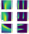 |
Fig. A.1. Cuts around the best solution in the χ2 cube obtained from MontAGN model 1. |
 |
Fig. A.2. Left: observed visibility. Right: visibility from MontAGN model 1. |
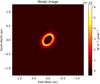 |
Fig. A.3. K-band image of the MontAGN model 1. The diffuse background is not represented. |
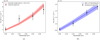 |
Fig. A.4. Spectral fits for MontAGN model 1. a: observed coherent spectrum and extincted model spectrum. b: diffuse background and temperature estimation. |
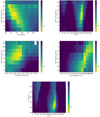 |
Fig. A.5. Cuts around the best solution in the χ2 cube obtained from MontAGN model 2. We note that the dust is not sampled linearly. |
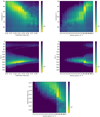 |
Fig. A.5. continued. |
 |
Fig. A.6. Left: observed visibility. Right: visibility from model 2. |
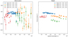 |
Fig. A.7. Left: observed closure phase. Right: closure phase from MontAGN model 2. |
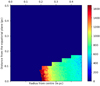 |
Fig. A.8. Temperature as a function of radius for the MontAGN model 2. |
Appendix B: Nuclear structures of NGC 1068
Comparison of the orientations observed for various substructures of the inner region of the NGC 1068 torus.
All Tables
Comparison of the orientations observed for various substructures of the inner region of the NGC 1068 torus.
All Figures
|
Fig. 1. u − v plane associated to the UT observation. (0) UT3–UT4, (1) UT2–UT4, (2) UT1–UT4, (3) UT2–UT3, (4) UT1–UT3, (5) UT1–UT2. |
| In the text | |
|
Fig. 2. Squared visibility color-coded according to baseline : (0) UT3–UT4, (1) UT2–UT4, (2) UT1–UT4, (3) UT2–UT3, (4) UT1–UT3, (5) UT1–UT2. |
| In the text | |
|
Fig. 3. Squared visibility color-coded according to wavelength (in meters), as listed in the legend. |
| In the text | |
|
Fig. 4. Closure phase color-coded per triplet. |
| In the text | |
|
Fig. 5. Observed coherent spectrum. |
| In the text | |
|
Fig. 6. a: image in arbitrary flux units of the best geometrical model, an elongated thick ring over-imposed on diffuse emission. b: comparison between the observed and the modeled visibilities. |
| In the text | |
|
Fig. 7. Geometry of the thick disk model used in the MontAGN simulations. The image is a cut along any direction orthogonal to the equatorial plane of the structure. |
| In the text | |
|
Fig. 8. Spectrum of the central source used in MontAGN simulations. |
| In the text | |
|
Fig. 9. Comparison between the observed visibility (left) and the one predicted by the MontAGN model 2 (right). |
| In the text | |
|
Fig. 10. Comparison between the observed closure phase (left) and the one predicted by the MontAGN model 2 (right). |
| In the text | |
|
Fig. 11. K-band image of the MontAGN model 2. The diffuse background is not represented. |
| In the text | |
|
Fig. 12. Spectral fits for model 2. a: observed coherent spectrum and extincted model spectrum. b: diffuse background and temperature estimation. |
| In the text | |
|
Fig. A.1. Cuts around the best solution in the χ2 cube obtained from MontAGN model 1. |
| In the text | |
|
Fig. A.2. Left: observed visibility. Right: visibility from MontAGN model 1. |
| In the text | |
|
Fig. A.3. K-band image of the MontAGN model 1. The diffuse background is not represented. |
| In the text | |
|
Fig. A.4. Spectral fits for MontAGN model 1. a: observed coherent spectrum and extincted model spectrum. b: diffuse background and temperature estimation. |
| In the text | |
|
Fig. A.5. Cuts around the best solution in the χ2 cube obtained from MontAGN model 2. We note that the dust is not sampled linearly. |
| In the text | |
|
Fig. A.5. continued. |
| In the text | |
|
Fig. A.6. Left: observed visibility. Right: visibility from model 2. |
| In the text | |
|
Fig. A.7. Left: observed closure phase. Right: closure phase from MontAGN model 2. |
| In the text | |
|
Fig. A.8. Temperature as a function of radius for the MontAGN model 2. |
| In the text | |
Current usage metrics show cumulative count of Article Views (full-text article views including HTML views, PDF and ePub downloads, according to the available data) and Abstracts Views on Vision4Press platform.
Data correspond to usage on the plateform after 2015. The current usage metrics is available 48-96 hours after online publication and is updated daily on week days.
Initial download of the metrics may take a while.