| Issue |
A&A
Volume 647, March 2021
|
|
|---|---|---|
| Article Number | A190 | |
| Number of page(s) | 15 | |
| Section | The Sun and the Heliosphere | |
| DOI | https://doi.org/10.1051/0004-6361/202039927 | |
| Published online | 05 April 2021 | |
Combining magneto-hydrostatic constraints with Stokes profiles inversions
II. Application to Hinode/SP observations
1
Leibniz-Institut für Sonnenphysik, Schöneckstr. 6, 79110 Freiburg, Germany
e-mail: This email address is being protected from spambots. You need JavaScript enabled to view it.
2
Institute for Solar Physics, Department of Astronomy, Stockholm University, AlbaNova University Centre, 10691 Stockholm, Sweden
3
Instituto de Astrofísica de Canarias, Avd. Vía Láctea s/n, 38205 La Laguna, Spain
4
Departamento de Astrofísica, Universidad de La Laguna, 38205 La Laguna, Tenerife, Spain
Received:
17
November
2020
Accepted:
16
December
2020
Abstract
Context. Inversion techniques applied to the radiative transfer equation for polarized light are capable of inferring the physical parameters in the solar atmosphere (temperature T, magnetic field B, and line-of-sight velocity vlos) from observations of the Stokes vector (i.e., spectropolarimetric observations) in spectral lines. Inferences are usually performed in the (x, y, τc) domain, where τc refers to the optical-depth scale. Generally, their determination in the (x, y, z) volume is not possible due to the lack of a reliable estimation of the gas pressure, particularly in regions of the solar surface harboring strong magnetic fields.
Aims. We aim to develop a new inversion code capable of reliably inferring the physical parameters in the (x, y, z) domain.
Methods. We combine, in a self-consistent way, an inverse solver for the radiative transfer equation (Firtez-DZ) with a solver for the magneto-hydrostatic equilibrium, which derives realistic values of the gas pressure by taking the magnetic pressure and tension into account.
Results. We test the correct behavior of the newly developed code with spectropolarimetric observations of two sunspots recorded with the spectropolarimeter (SP) instrument on board the Hinode spacecraft, and we show how the physical parameters are inferred in the (x, y, z) domain, with the Wilson depression of the sunspots arising as a natural consequence of the force balance. In particular, our approach significantly improves upon previous determinations that were based on semiempirical models.
Conclusions. Our results open the door for the possibility of calculating reliable electric currents in three dimensions, j(x, y, z), in the solar photosphere. Further consistency checks would include a comparison with other methods that have recently been proposed and which achieve similar goals.
Key words: sunspots / Sun: magnetic fields / Sun: photosphere / polarization / magnetohydrodynamics (MHD)
© ESO 2021
1. Introduction
Inversion techniques applied to the radiative transfer equation for polarized light are arguably the best tools at our disposal for inferring the physical properties (temperature T, magnetic field B, and line-of-sight velocity vlos) of the solar atmosphere (Socas-Navarro 2001; del Toro Iniesta 2003a; Bellot Rubio et al. 2006; Ruiz Cobo et al. 2007; del Toro Iniesta & Ruiz Cobo 2016). Because the natural scale to describe how photons propagate is the so-called optical depth (τ), the physical properties are inferred in the (x, y, τc), where τc refers to the continuum optical depth. Here “continuum” means any wavelength where the absorption is only due to bound-free and free-free transitions (Mihalas 1970, Sect. 4.4).
In order to infer the physical parameters in the (x, y, z) domain, additional constraints must be invoked. By far, the most widely used has been hydrostatic equilibrium. However, this assumption is adequate only in regions where the magnetic field is force-free (i.e., Lorentz force ∝j × B = 0) and the plasma is stationary (i.e., no time dependence) and static (i.e., no velocities). In many regions of the solar atmosphere, notably in sunspots, the force-free assumption breaks down and a different method must therefore be employed.
The first authors that attempted a more realistic treatment were Martinez Pillet & Vazquez (1990, 1993), Solanki et al. (1993). They all employed the theoretical model from Maltby (1977), which considers an axially symmetric magnetic field around the sunspot in order to account for the magnetic pressure and tension. This approach had been used until recently (see e.g., Mathew et al. 2004), until the pioneering work of (Puschmann et al. 2010, hereafter referred to as PUS2010), who presented a new method based on the minimization of the Lorentz force and ∇ ⋅ B in order to transform the physical parameters from the (x, y, τc) domain into the (x, y, z) domain. Despite its importance, PUS2010 suffers a couple of drawbacks. The first is that the minimization, based on a genetic algorithm, is very slow due to the large number of free parameters and therefore can only deal with relatively small regions. More important, however, is the fact that the gas pressure is modified in the process of inferring the physical parameters in the (x, y, z) domain, and therefore the physical parameters are not able to provide the best possible fit to the observed polarization signals.
The results from PUS2010 have sparked a new interest in developing an inversion code for the radiative transfer equation that is capable of inferring the physical parameters in the solar atmosphere in the geometrical (x, y, z) three-dimensional domain. This has resulted in a number of new approaches, beginning with adapting the PUS2010 method to minimize only ∇ ⋅ B but in a much larger area (Löptien et al. 2018, 2020). Methods that rely on magneto-hydrodynamic (MHD) simulations have also been developed, with some using these simulations as training sets for artificial neural networks (Carroll & Kopf 2008) and convolutional neural networks (Asensio Ramos & Díaz Baso 2019), while others employing them as a database of physical parameters capable of fitting the observed polarization signals (Riethmüller et al. 2017).
We have developed an alternative approach that is loosely based on PUS2010. In Pastor Yabar et al. (2019), we presented an inversion code for the radiative transfer equation that works directly in the (x, y, z) domain, and we showed that the reliability of inferences in the z-scale depend upon the realism of the gas pressure (Pg). In Borrero et al. (2019), we presented a method that is based on the magneto-hydrostatic (MHS) equilibrium instead of hydrostatic equilibrium and can be used to infer very realistic values of Pg. In this article, we come full circle and demonstrate how the approaches presented in the previous two papers can be combined to determine accurate physical parameters in the solar atmosphere in the (x, y, z) domain, by applying our newly developed methods to spectropolarimetric observations with high spatial and spectral resolution.
2. Hinode/SP observations
The observations employed in this work correspond to spectropolarimetric observations (i.e., Stokes vector 𝕀obs) of two neutral iron (Fe I) spectral lines at 630 nm. The Stokes vector possesses four components, 𝕀 = (I, Q, U, V), where I refers to the total intensity, Q and U to the linear polarization, and V to the circular polarization (see Sect. 3.3 in del Toro Iniesta 2003b).
The observations were carried out with the spectropolarimeter (SP; Lites et al. 2001; Ichimoto et al. 2007) attached to the Solar Optical Telescope (SOT; Suematsu et al. 2008; Tsuneta et al. 2008; Shimizu et al. 2008) on board the Japanese satellite Hinode (Kosugi et al. 2007). The spectral region containing the two aforementioned Fe I lines was measured across Λ = 112 wavelength points with a wavelength sampling of about 21.5 mÅ. The atomic parameters for these spectral lines can be found in Borrero et al. (2014) (see their Table 1). The SP is a slit-spectrograph where a given region is scanned spatially. For each slit position, the light is integrated for a total of 4.8 s, yielding a noise level of σ = 10−3 in units of the quiet-Sun continuum intensity. The spatial sampling along the slit and perpendicular to it is about 0.16 arcsec (i.e., dx = dy = 120 km at disk center).
In this work, we analyze spectropolarimetric data from two different sunspots: NOAA AR 10923 and NOAA AR 10944. Both spots were observed very close to disk center μ ≈ 1.0, on November 14, 2006 (at around 7:15 UT) and February 28, 2007 (at around 11:50 UT), respectively. Maps of the continuum intensity Ic, normalized to the quiet-Sun continuum intensity Ic, qs, can be seen in Fig. 1 for AR 10923 (left) and AR 10944 (right). The analyzed maps possess the following horizontal dimensions (in pixels): L = 645, M = 640 and L = 350, M = 300, respectively.
 |
Fig. 1. Maps of the normalized continuum intensity, Ic/Ic, qs, for the two sunspots analyzed in this work. Left: NOAA AR 10923 observed on November 14, 2006. Right: NOAA AR 10944 observed on February 28, 2007. At the time of the observations, both sunspots were located at disk center. Regions marked with red symbols and solid blue lines will be studied in more detail later on. |
3. Methodology
3.1. Stokes inversion with Firtez-DZ
The Stokes inversion code employed in this work is Firtez-DZ (Pastor Yabar et al. 2019). A graphical sketch of how Firtez-DZ operates is presented in Fig. 2 and is highlighted in red boxes. A more detailed description of this figure will be given throughout this section. Firtez-DZ needs guesses of the physical parameters 𝒞ij in the solar atmosphere as inputs. We refer to these physical parameters with the super-indexes i, j, where i-even indicates that we are currently inside the Stokes inversion loop within Firtez-DZ, while i-odd implies that we are inside the MHS module. Index j stands for the iteration number within either Firtez-DZ or the MHS module and is reset to j = 0 every time the Stokes inversion and MHS modules communicate with each other.
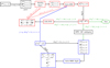 |
Fig. 2. Flow chart indicating the inversion process of the radiative transfer equation (RTE) for polarized light (i.e., the Stokes inversion) combined with MHS constraints. The black squares denote the acquisition of the observed Stokes vector 𝕀obs(x, y, λ) and the determination of an initial set of physical parameters (T00(x, y, z), B00(x, y, z)) with which we can start the inversion (i.e., a guess). The red squares indicate the inversion process as carried out by the Firtez-DZ code. This is described in detail in Sect. 3.1. Blue squares correspond to the steps carried out by the MHS module (see Sect. 3.3 for details). Finally, green squares and arrows indicate locations where an interplay between Firtez-DZ and the MHS module are needed in order to assess if convergence and exit conditions are achieved (see Sect. 3.4 for more information). |
The aforementioned physical parameters 𝒞ij stand for: temperature (Tij), three components of the magnetic field ( ,
,  ,
,  ), and the line-of-sight component of the velocity (
 ), all as a function of the Cartesian1 coordinates (x, y, z). Besides these physical parameters, Firtez-DZ needs the density ρij and gas pressure
  . The former can be obtained from the latter if the temperature is known by using the equation of state:
 (1)
(1)
where u and Kb refer to the atomic unit mass and the Boltzmann constant, respectively: u = 1.6605 × 10⁻²⁴ g and Kb = 1.3806 × 10⁻¹⁶ erg K−1. The mean molecular weight μ is a function of T and Pg, and its determination involves the iterative computation of the Saha ionization equation and the Boltzmann equation for the occupancy of the energy levels within an atom (Mihalas 1970).
The question that remains is how to determine the gas pressure  at every j-step during the inversion process. At i = 0, the MHS module has not yet been employed, so we need to rely on hydrostatic equilibrium approximation along the vertical direction:
 (2)
(2)
where g = 2.74 cm s−2 is the Sun’s gravitational acceleration. The gas pressure is recalculated at every j-step during the Stokes inversion as long as i = 0 (i.e., hydrostatic equilibrium). This is indicated by the solid red arrow in Fig. 2. For i ≥ 1, the MHS module (Sect. 3.3) already provides the gas pressure, and therefore we do not need to calculate it. Indeed, for i ≥ 1, Firtez-DZ keeps Pg constant during the Stokes inversion (i.e., j-step; see dashed red arrow in Fig. 2).
With all these ingredients, Firtez-DZ solves the radiative transfer equation for polarized light in the z-scale (Landi Degl’Innocenti & Landi Degl’Innocenti 1985) under the assumption of local thermodynamic equilibrium and computes the polarized spectrum (i.e., Stokes vector 𝕀ij) of atomic spectral lines in the Zeeman regime as a function of wavelength and horizontal grid position (x, y, λ). This Stokes vector is referred to as a “synthetic” Stokes vector and is denoted as  . The four components of the Stokes vector (see Sect. 2) are generically referred to as Is, ij (Is = 1 = I, Is = 2 = Q, Is = 3 = U, Is = 4 = V). The
  is then compared to the observed Stokes vector 𝕀obs(x, y, λ) via a χ2-merit function:
![Mathematical equation: $$ \begin{aligned} \chi ^2({\mathbb{I} }^\mathrm{syn}_{ij},{\mathbb{I} }^\mathrm{obs})&= \frac{1}{4ML\Lambda -F} \sum \limits _{l=1}^{L}\sum \limits _{m=1}^{M} \sum \limits _{k=1}^{\Lambda }\sum \limits _{s=1}^4 { w}_s^2 [I_s^\mathrm{obs}(x_l,{ y}_m,\lambda _k)\nonumber \\&\quad -I_{s,ij}^\mathrm{syn}(x_l,{ y}_m,\lambda _k)]^2 \;\;{\mathrm{with}\,i\,\mathrm{even}}, \end{aligned} $$](/articles/aa/full_html/2021/03/aa39927-20/aa39927-20-eq11.gif) (3)
(3)
where the sum runs for all grid points on the horizontal plane (x, y) (indexes l and m, respectively), for all observed wavelengths (index k) and for all four Stokes parameters (index s). In order to help the reader keep track of all indexes, a summary is provided in Table 1. In Eq. (3), F stands for the total number of free parameters employed in the inversion (see Table 2). The ws factors in Eq. (3) are used as weights during the inversion of the radiative transfer equation (see Eq. (35) del Toro Iniesta & Ruiz Cobo 2016), and χ2 is normalized such that a value of χ2 < 1 indicates a good fit between 𝕀obs and  . In this paper, the inversion is performed such that it gives three times more weight to the linear polarization profiles Q and U than to I: w2 = w3 = 3w1, and two times more weight to the circular polarization V than to I: w4 = 2w1. The weight given to Stokes I was taken as the inverse of the noise (see Sect. 2): w1 = 1/σ.
Analytical derivatives of χ2 with respect to the physical parameters2 are calculated and fed into a Levenberg-Marquardt (LM) algorithm (Press et al. 1986) that, along with the singular decomposition value (SVD) method (Golub & Kahan 1965), provides the new physical parameters in the solar atmosphere 𝒞ij + 1 as a function of (x, y, z); these new parameters produce a better match between the synthetic and observed Stokes profiles:  . This process continues iteratively until the best possible match between the synthetic and observed Stokes vector is found (i.e., χ2-minimization).
We will now assume that the minimization is achieved after j = p iterations of the Stokes inversion process (i-even), thus proving the physical parameters in the solar atmosphere, ![Mathematical equation: $ [{\mathcal{C}}^{ip}, P_{\mathrm{g}}^{ip}, \rho^{ip}] $](/articles/aa/full_html/2021/03/aa39927-20/aa39927-20-eq16.gif) , as a function of (x, y, z). If i = 0, Firtez-DZ provides only a “first estimation” of the physical parameters in the solar atmosphere as a function of (x, y, z) because, as discussed in Pastor Yabar et al. (2019), their reliability in the (x, y, z) domain depends upon the accuracy of the gas pressure Pg(x, y, z), whose inference is in turn hindered by the limitations of hydrostatic equilibrium employed at i = 0. In order to improve the determination of Pg(x, y, z), all physical parameters (Tip,
, as a function of (x, y, z). If i = 0, Firtez-DZ provides only a “first estimation” of the physical parameters in the solar atmosphere as a function of (x, y, z) because, as discussed in Pastor Yabar et al. (2019), their reliability in the (x, y, z) domain depends upon the accuracy of the gas pressure Pg(x, y, z), whose inference is in turn hindered by the limitations of hydrostatic equilibrium employed at i = 0. In order to improve the determination of Pg(x, y, z), all physical parameters (Tip,  , ρip,
  ,
,  ,
,  , and
, and  ) are then passed onto the disambiguation module (Sect. 3.2) and from there to the MHS module (Sect. 3.3). With this, we increase the i-index by one (i is now odd), and, since the MHS module has its own internal iteration that is independent from the Stokes inversion, we also reset the j-index to zero. This step is indicated by the green arrow in Fig. 2.
During the inversion process, the three-dimensional volume is discretized in L, M, and N points along each of the three Cartesian coordinates, x, y, and z, respectively. The grid sizes are denoted as dx, dy, and dz. In all our inversions, we discretized the vertical direction with N = 128 grid points with a spacing of dz = 12 km. The number of grid points on the horizontal plane, L and M, depends on the actual size of the observed sunspots (see Sect. 2). The horizontal spacing is always dx = dy = 120 km. A summary of these values is also included in Table 1.
We note that the inversion process performed by Firtez-DZ is done in such a way that the complexity of the atmospheric model along the vertical z-direction increases slowly. This means that the number of free parameters that are determined, at every j-step of the Stokes inversion process (i-even), also increases. More details can be found in Pastor Yabar et al. (2019, see Sect. 2.3). The number of free parameters employed in this paper is indicated in Table 2.
We slightly modified the original implementation of Firtez-DZ in order to avoid excessively modifying the temperature outside the “sensitivity region”, which we denote as [τa, τb] (τa > τb; see also Appendix A). To do so, temperature perturbations δT, calculated with the LM algorithm, are forced to exponentially decay above τb:
![Mathematical equation: $$ \begin{aligned} \delta T(z) = \delta T(z[\tau _{i}])\,exp\{-2(\log \tau _{b}-\log \tau _{i})\} \;\; \text{if} \;\; z < z(\tau _b) . \end{aligned} $$](/articles/aa/full_html/2021/03/aa39927-20/aa39927-20-eq22.gif) (4)
(4)
Additionally, temperature perturbations for layers below τa are set to be equal to those at the sensitivity region limit, namely: δT(z) = δT(z[τa]) if z > z(τa).
3.2. Disambiguation module
Between the inversion of the radiative transfer equation (Sect. 3.1; i-even) and the MHS module (Sect. 3.3; i-odd), there is an intermediate step that refers to the resolution of the 180° ambiguity on the horizontal component of the magnetic field. As already mentioned in Borrero et al. (2019) (Sect. 5), the inversion of the radiative transfer equation provides the horizontal component of the magnetic field (Bx, By) with an ambiguity of 180° (Metcalf 1994). This means that, at every point on the solar surface (x, y), we could randomly exchange (Bx, By, Bz) with (− Bx, −By, Bz) and the radiative transfer equation would yield exactly the same solution: 𝕀syn(x, y, λ). If the magnetic field thus inferred is fed into the MHS module (Sect. 3.3), we would solve for a completely erroneous force balance as the electric currents derived from such a magnetic field, j = (4π)−1c∇ × B, would be completely unrealistic.
Therefore, we first must ensure that the aforementioned ambiguity has been resolved. While there are many tools available to solve this issue (Metcalf et al. 2006), we decided to employ the so-called non-potential field calculation method (NPFC) from Georgoulis (2005). Since the NPFC method works in a two-dimensional plane parallel to the solar surface (i.e., fixed z), we solved the 180° ambiguity at the height z that corresponds to the middle of the sensitivity region for the magnetic field  , where
  is defined in Eq. (A.2). This is where it makes the most sense to solve the 180° ambiguity as it is the region where the errors in the inference of B by Firtez-DZ are the smallest. Elsewhere, we simply extrapolated the solution from the NPFC method to all other z values.
3.3. Magneto-hydrostatic module
The MHS module receives the physical parameters from the disambiguation module. This is indicated by the green arrow in Fig. 2. The MHS module is based on the approach presented in Borrero et al. (2019). In that paper, we employed the “fishpack” library (Swarztrauber & Sweet 1975) to solve the following equation, which represents the MHS equilibrium in the solar atmosphere:
 (5)
(5)
In this paper, we employed the magnetic field inferred from the inversion of the radiative transfer equation. This is not necessarily consistent with the MHD equations and contains measurement errors (see e.g., Wiegelmann & Inhester 2010). Therefore, we solved a modified version of Eq. (5), namely
![Mathematical equation: $$ \begin{aligned} \nabla ^2 (\ln P_{\rm g}) = -\frac{g u}{K_{\rm b}} \frac{\partial }{\partial z}\left(\frac{\mu }{T}\right) - \frac{f(\beta )}{c P_{\rm g}}\left[\frac{4\pi \Vert \boldsymbol{j}\Vert ^2}{c}+(\boldsymbol{j} \times \boldsymbol{B}) \cdot \boldsymbol{\nabla }(\ln P_{\rm g})\right] . \end{aligned} $$](/articles/aa/full_html/2021/03/aa39927-20/aa39927-20-eq26.gif) (6)
(6)
The derivation of this equation is detailed in Appendix B. Here we only need to mention that the factor f(β) is a function that aims at limiting the effect of the Lorentz force in those regions of the solar atmosphere where the plasma-β, defined as β = 8πPg/∥B∥2, drops below a certain value β*. We prescribe f(β) as:
 (7)
(7)
where we adopt β* = 0.5. Using a first estimation of the gas pressure  (i-odd), we can solve for the left-hand side of Eq. (6) as a Poisson-like equation and obtain a new gas pressure,
  , which is then inserted back into the right-hand side, and the process continues until convergence. Each time a new gas pressure is obtained, the conversion between z and the optical depth τc changes even if the temperature is kept constant (see Appendix A and Eq. (A.1)). Convergence is assessed by requiring that the Wilson depression zw = z(τc = 1) does not vary, on average over the observed region, by more than half a vertical grid point (dz/2) between two consecutive iterations. To this end, we defined the following χ2-merit for the Wilson depression:
![Mathematical equation: $$ \begin{aligned} \chi ^2(z_{ w}^{ij+1},z_{ w}^{ij})&= \frac{1}{LM \mathrm{d}z^2} \sum \limits _{l=1}^L\sum \limits _{m=1}^M [z^{ij+1}(x_l,{ y}_m,\tau _{\rm c}=1) \nonumber \\&\quad - z^{ij}(x_l,{ y}_m,\tau _{\rm c}=1)]^2 \;\;{\mathrm{with}\,i-\mathrm{odd}}. \end{aligned} $$](/articles/aa/full_html/2021/03/aa39927-20/aa39927-20-eq30.gif) (8)
(8)
With the previous conditions, convergence is achieved whenever  . The iterations performed by the MHS module are illustrated in Fig. 2 in blue boxes. We will now assume that convergence occurs after j = q iterations, resulting in a gas pressure
  with i-odd. The resulting physical parameters
 ![Mathematical equation: $ [{\mathcal{C}}_{\dagger}^{iq},P_{\mathrm{g}}^{iq},\rho^{iq}] $](/articles/aa/full_html/2021/03/aa39927-20/aa39927-20-eq33.gif) are then sent back into the Stokes inversion module by Firtez-DZ (Sect. 3.1). We then increase the i-index by one, which thus becomes an even number, and again we reset the j-index to zero. This is indicated by the blue arrow in Fig. 2.
are then sent back into the Stokes inversion module by Firtez-DZ (Sect. 3.1). We then increase the i-index by one, which thus becomes an even number, and again we reset the j-index to zero. This is indicated by the blue arrow in Fig. 2.
It is important to note here that the physical parameters 𝒞† that the MHS module sends back to the Firtez-DZ inversion code (blue arrow in Fig. 2) are not exactly the same as the physical parameters 𝒞 that the MHS module receives from Firtez-DZ (green arrow in Fig. 2). This occurs because even though C and 𝒞† are the same in the (x, y, z) domain, they might differ significantly in the (x, y, τc) scale as the conversion between z and τc is strongly dependent on the gas pressure and density (see Eq. (A.1)).
Finally, it must be borne in mind that, in order to solve Eq. (6), we need to establish a number of boundary conditions for the gas pressure Pg on the left-hand side of this equation, as well as for the magnetic field and temperature on the right-hand side. The boundary conditions employed in this work are detailed in Appendix C.
3.4. Iterating between Firtez-DZ and the MHS module
As mentioned in Sect. 3.1, the inversion code Firtez-DZ iteratively determines (i-even; see red boxes in Fig. 2) the temperature, T, the vertical component of the velocity, vz, and three components of the magnetic field, Bx, By, and Bz, in the three-dimensional (x, y, z) domain. These physical parameters were referred to as 𝒞. The gas pressure Pg was initially (i = 0) determined under hydrostatic equilibrium (Eq. (2)), while the density, ρ, is determined by applying the equation of state (Eq. (1)). All these parameters (𝒞, Pg, and ρ) are then passed through the disambiguation module and onto the MHS module so as to determine a more consistent gas pressure through the iterative solution of Eq. (6) (i-odd; see blue boxes in Fig. 2).
At this point, at i = 0, or in other words before the MHS module has been applied even once, we calculate the gas pressure and density through hydrostatic equilibrium (Eq. (2)). Because ρ depends on the temperature through Eq. (1), we need to reevaluate Eq. (2) at every step of the j-index iteration (Firtez-DZ). That is why in Fig. 2, after the temperature is modified, T0 j + 1 = T0j + δT0j, we go back to Eq. (2) (see solid red arrow). However, after the application of the MHS module (i ≥ 1), the physical parameters are directly employed to solve the radiative transfer equation inside Firtez-DZ (blue arrow in Fig. 2). In fact, for i ≥ 1, the gas pressure is never modified by Firtez-DZ and is kept to whatever values came from the MHS module (dashed red arrow in Fig. 2; see also Sect. 3.1). The density, however, does change inside Firtez-DZ because the temperature is being changed by the LM and SVD algorithms (LM+SVD box in Fig. 2).
Finally, we note that, as mentioned in Sect. 3.3, the physical parameters  that come out of the MHS module and are fed back into the Firtez-DZ are in general different from those inferred from the inversion code. Consequently, the output physical parameters from the MHS module, 𝒞iq (i-odd), will not necessarily produce the same 𝕀syn as the output physical parameters 𝒞ip (i-even) from Firtez-DZ. As indicated by the green if-statements in Fig. 2, Firtez-DZ verifies this by measuring whether the physical parameters from the MHS module, 𝒞iq, can still produce a good fit to 𝕀obs. If they cannot, Firtez-DZ resumes the inversion while keeping the gas pressure fixed at
  (i-odd). On the other hand, if 𝒞iq does indeed produce a good fit to 𝕀obs, we can consider that we have achieved convergence in both Firtez-DZ and the MHS module, and we therefore exit the process.
4. Fits to observed data
As mentioned in Sect. 1, one of the limitations in PUS2010 was that the resulting synthetic Stokes profiles, 𝕀syn(x, y, λ), did not provide the best possible fit to the observed ones, 𝕀obs(x, y, λ). This was more a matter of choice rather than a real limitation. The optimization process in PUS2010, based on a genetic algorithm, was too time-consuming to allow for further iterations in the inversion process. Aside from this, there was nothing preventing those authors from feeding their results in the z-scale back into the Stokes inversion code in order to continue the χ2-minimization (Eq. (3)). This is explicitly taken into account in our method, as already explained in Sect. 3.4 and illustrated in Fig. 2. Therefore, our method can be considered as having a similar motivation as those from Riethmüller et al. (2017) and Löptien et al. (2018), in the sense that we aim at providing the best possible fit to the observed Stokes profiles. This is in contrast with PUS2010 and Asensio Ramos & Díaz Baso (2019), where fitting the observations plays a secondary role.
To showcase the quality of the fits, we present, in Figs. 3–5, three examples – in the umbra, penumbra, and quiet Sun, respectively – of the observed Stokes profiles (black dots) and the best-fit profiles (solid colored lines) after i = 0 (orange), i = 2 (green), i = 4 (red), and i = 6 (purple). These examples provide only a qualitative idea about the quality of the fits. A more quantitative picture can be drawn from Fig. 6, where we present the mean value of  over the entire field-of-view for NOAA AR 10944 (blue; right-hand panel in Fig. 1) and NOAA AR 10923 (orange; left-hand panel in Fig. 1). As can be seen, i = 6 yields the best fits of the observed profiles. We note that this is simply a side effect of having the largest number of free parameters (see Table 2). This case allows us to fit even well-known asymmetric Stokes V profiles found in the sunspot penumbra, as seen in Fig. 4 (see also Sanchez Almeida & Lites 1992; Borrero et al. 2006). The important thing to consider here is not that the fit improves for larger i values, but rather that it does not get worse. The reason is that the pressure and density, and hence also the optical-depth scale, are modified after each application of the MHS module (i-odd; see Sect. 3.3), thus potentially changing the synthetic profiles 𝕀syn(x, y, λ) in a way that they no longer provide the best fit to the observed Stokes vector 𝕀obs(x, y, λ) (see e.g., Fig. 9 in PUS2010).
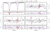 |
Fig. 3. Observed (black dots) and best-fit Stokes profiles (solid lines) after the application of the Firtez-DZ inversion code (i-even): i = 0 (orange), i = 2 (green), i = 4 (red), and i = 6 (purple). The spatial location of these profiles corresponds to a quiet-Sun pixel (red diamond in the right-hand panel of Fig. 1.) The intensity as a function of wavelength I(λ), normalized to the average quiet-Sun continuum intensity Ic, qs, in the two Fe I lines at 630 nm is presented in the upper-left panel. The linear polarization profiles, Q(λ) and U(λ), are displayed in the upper-right and lower-left panels, respectively. Finally, the circular polarization profile, V(λ), is shown in the lower-right panel. |
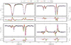 |
Fig. 4. Same as Fig. 3 but for a pixel located in the penumbra (see the red triangle in the right-hand panel of Fig. 1). |
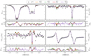 |
Fig. 5. Same as Fig. 3 but for a pixel located in the umbra (see the red square in the right-hand panel of Fig. 1). |
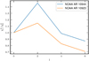 |
Fig. 6. Mean value of the χ2-merit function between the observed 𝕀obs(x, y, λ) and synthetic 𝕀syn(x, y, λ) Stokes profiles (Eq. (3)) over the entire field-of-view as a function of the inversion iteration (i-even) performed with the Firtez inversion code (Sect. 3.1). Results for NOAA AR 10944 (left-hand panel in Fig. 1) are indicated in orange, while results for NOAA AR 10944 (right-hand panel in Fig. 1) are shown in blue. |
5. Inferred physical parameters
Next we look at the physical parameters inferred from the combined application of the Firtez-DZ inversion code (Sect. 3.1) and the MHS constraints (Sect. 3.3). While the physical parameters are retrieved in the (x, y, z) domain, we will not consider those regions outside [z(τa),z(τb)], where τa = 10 and τb = 10−4. As such, we avoid presenting results in atmospheric layers where the errors are large. As explained in Appendix A, the locations of z(τa) and z(τb) depend on the point of the solar surface (x, y) where we look. This can be illustrated by plotting the physical parameters in the XZ plane for a fixed value of y (see horizontal blue lines in Fig. 1). These physical parameters are presented in Figs. 7 and 8 for NOAA AR 10923 and 10944, respectively. In these figures, we present the absolute value of the vertical component of the magnetic field ∥Bz(x, z) ∥ (first panel), the radial component of the magnetic field ![Mathematical equation: $ B_{\rm r}(x,z) = [B_x^2(x,z)+B_{\it y}^2(x,z)]^{1/2} $](/articles/aa/full_html/2021/03/aa39927-20/aa39927-20-eq37.gif) (second panel), the temperature T(x, z) (third panel), and the logarithm of the gas pressure log Pg(x, z) (fourth panel). We note that NOAA AR 10923 is a negative polarity sunspot (Bz < 0 in the umbra) but that this is not seen because we plot only ∥Bz(x, z)∥. Another important point is that the vertical z-scale and horizontal x-scale are not identical in these figures. While the total vertical extension of the box is about 1.5 Mm, it horizontally covers 40–60 Mm (see Sect. 3 and Table 1). Therefore, for a better visualization, we have stretched the vertical z-scale.
(second panel), the temperature T(x, z) (third panel), and the logarithm of the gas pressure log Pg(x, z) (fourth panel). We note that NOAA AR 10923 is a negative polarity sunspot (Bz < 0 in the umbra) but that this is not seen because we plot only ∥Bz(x, z)∥. Another important point is that the vertical z-scale and horizontal x-scale are not identical in these figures. While the total vertical extension of the box is about 1.5 Mm, it horizontally covers 40–60 Mm (see Sect. 3 and Table 1). Therefore, for a better visualization, we have stretched the vertical z-scale.
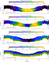 |
Fig. 7. Physical parameters for the sunspot NOAA AR 10923 on a vertical slice (XZ-plane) along the blue line in Fig. 1 (left-hand panel). From top to bottom: vertical component of the magnetic field Bz, radial component of the magnetic field Br, temperature T, and logarithm of the gas pressure Pg. The solid black line indicates the location of the Wilson depression (z(τc = 1) level). See the text for more details. |
In Figs. 7 and 8, the solid black lines indicate the location of z(τc = 1) (i.e., the Wilson depression). In these figures, we can see that, along the selected slice of constant y (blue lines in Fig. 1), the location of z(τc = 1) is about z ≈ 1.0 Mm in the quiet Sun, whereas in the umbra it decreases to about z ≈ 0.4−0.5 Mm, yielding a Wilson depression of some 500–600 km. We can also notice many small-scale features. Two examples of such features are umbral dots and/or light bridges (vertical dashed line in Fig. 8 at x ≈ 21 Mm), where we see a local enhancement in the temperature T and a local decrease in Bz at around z ≈ 0.5 Mm. This is accompanied by a small increase in the location of the z(τc = 1) level. Other interesting features are the magnetic field concentrations and magnetic knots outside the sunspot. They are seen, for instance, at x ≈ 75 Mm in Fig. 7 (see the vertical dashed lines). These magnetic knots are characterized by having strong vertical magnetic fields of the same or opposite polarity of the sunspot’s magnetic field, and they feature a strong dip at the z(τc = 1) level.
In Figs. 9 and 10, we show the two-dimensional (x, y) maps of the geometrical height at which different τc levels are reached in NOAA AR 10923 and 10944, respectively. All values are given with respect to the quiet Sun zqs(τc) (see white rectangles in these figures). These maps correspond to four different realizations of the z − τc conversion (see Eq. (A.1)) over the entire observed regions. Again, our method is capable of inferring the small-scale structure of the conversion between geometrical height z and optical depth τc. This is clearly seen around the light bridges in both sunspots as well as the magnetic knots around them. The mean values of the Wilson depression, zqs(τc = 1)−z(τc = 1), in the umbra obtained with our method are 588 km for NOAA AR 10923 (Fig. 9; upper-left panel) and 524 km for NOAA A 10944 (Fig. 10; upper-left panel). The maximum values around are 630 and 580 km, respectively.
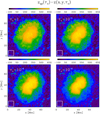 |
Fig. 9. Maps of the geometrical height at which different τc levels are reached in NOAA AR 10923: τc = 1 (top left), τc = 10−1 (top right), τc = 10−2 (bottom left), and τc = 10−3 (bottom right). All values are given with respect to the geometrical height for that τc level in the quiet Sun, zqs(τc). The quiet-Sun value is calculated as the spatial average over the white rectangle. |
It is important to notice that panels for each τc level differ. This is a consequence of our method being capable of stretching and/or shrinking the z − τc scale between consecutive grid points along the vertical direction through the changes in temperature, density, and pressure (see Eq. (A.1)). Other methods, where the z − τ conversion is obtained by simply shifting, at each (x, y)-location, the entire z-scale up or down, would yield exactly the same results at different τc levels in Figs. 9 and 10.
6. Conclusions
We have presented a new inversion code for the polarized radiative transfer equation that is capable of retrieving the physical parameters in the solar photosphere in the (x, y, z) domain in a way that is consistent with the MHS equations, and therefore it takes into account the effects of the Lorentz force (magnetic tension and pressure) in the force balance. Because of this, our new inversion code is capable of inferring not only the three components of the magnetic field, the temperature, and the line-of-sight velocity, but also the gas pressure and density in the solar photosphere. The development of this code is inspired, albeit loosely, on the work by Puschmann et al. (2010).
The inversion code makes use of the Firtez-DZ code and an MHS solver that have been described and tested separately by Pastor Yabar et al. (2019) and Borrero et al. (2019), respectively, employing results from three-dimensional MHD simulations of sunspots (Rempel 2012). In this paper, we combine both approaches into a single one and test its results with spectropolarimetric observations from the Hinode/SP instrument in two sunspots located very close to disk center.
To put our new approach in context, we will categorize all available methods (Carroll & Kopf 2008; Puschmann et al. 2010; Riethmüller et al. 2017; Löptien et al. 2018; Asensio Ramos & Díaz Baso 2019) that also aim at retrieving the physical parameters in the (x, y, z) domain into those that: (a) can be applied to large regions of the solar surface (i.e., entire sunspots plus their surrounding plage, moat, and quiet Sun); (b) infer the small-scale structure (i.e., umbral dots, penumbral filaments, light bridges, magnetic knots, etc.); and (c) fit the observed Stokes vector. All of the aforementioned methods give priority to some features at the expense of others. For instance, Löptien et al. (2018) limit the number of Fourier coefficients in order to analyze large fields-of-view, thereby limiting their ability to retrieve small-scale structures. Puschmann et al. (2010) make the opposite sacrifice. The Asensio Ramos & Díaz Baso (2019) method can deal with both situations but does not provide the best possible fit to the observed Stokes vector. Although our method meets the three previous requirements, there is a very obvious drawback: its speed. Just to give some numbers: the first iteration cycle (i = 0) took totals of 500 (small spot) or 2000 (large spot) combined CPU (central processing unit) hours. Later iterations (i ≥ 2) needed about half this. Although the actual running time was significantly reduced by running our inversions in clusters with several hundred nodes, our method is not yet suitable for processing large amounts of data. Therefore, which of the available methods is to be preferred depends on the particular use case.
Our inversion code also yields, in a natural way, the Wilson depression across the solar surface, not only at τc = 1 but at all optical depths within the region where the analyzed spectral lines are formed. Our values for the inferred Wilson depression are compatible, albeit somewhat smaller, by about 50–70 km, with similar studies of the same sunspots (Löptien et al. 2018, 2020; Asensio Ramos & Díaz Baso 2019). We note, however, that those studies were carried out with inversion results that considered the effects of the telescope and instrument point spread function (PSF). Those inversions usually retrieve sharper variations of the magnetic field along the (x, y)-directions, which is likely the reason our results differ from theirs. We will study this particular point in more detail in a future work by implementing the coupled-inversion technique by van Noort (2012) into our code, in order to remove the smearing effects introduced by the instrumental PSF.
It is also desirable to check how close to solenoidal the inferred magnetic field B(x, y, z) is. This might imply the implementation of a new approach, within our inversion code, to minimize ∇ ⋅ B. Therefore, we have decided to leave it for a future study. Such minimization seems to help improve the results of the inferences in the (x, y, z) domain (Puschmann et al. 2010; Löptien et al. 2018). We are not sure, however, how much our method will benefit from such an implementation as methods that minimize ∇ ⋅ B typically only modify the potential component of the magnetic field while leaving the non-potential component, and hence the electric currents j ∝ ∇ × B, untouched (Tóth 2000). Consequently, none of those methods would have any effect on the MHS force balance as implemented in our code (Eq. (6); Appendix B).
A corollary of the discussion in the previous paragraph is that, in its current state, our inversion code can be used to infer realistic electric currents j even if the magnetic field is not close to being solenoidal. We foresee future applications where the full j-vector, instead of simply its vertical jz-component, is employed to study the evolution of magnetic structures on the solar surface that are likely to produce enhanced chromospheric and coronal activity (see e.g., Solanki et al. 2003; Wang et al. 2017).
In this paper we will always assume that the observer’s line-of-sight is parallel to the gravity direction −z and therefore vlos = vz. This is possible because the selected observations are very close to disk center (μ ≈ 1; see Sect. 2).
These derivatives are ultimately written as a function of the derivatives of the Stokes vector with respect to the physical parameters: the so-called response functions (see Sect. 6 in del Toro Iniesta & Ruiz Cobo 2016).
Acknowledgments
This work has received funding from the Deutsche Forschungsgemeinschaft (DFG project number 321818926) and from the European Research Council (ERC) under the European Union’s Horizon 2020 research and innovation programme (SUNMAG, grant agreement 759548). JMB acknowledges travel support from the Spanish Ministry of Economy and Competitiveness (MINECO) under the 2015 Severo Ochoa Program MINECO SEV-2015-0548 and from the SOLARNET project that has received funding from the European Union’s Horizon 2020 research and innovation programme under grant agreement no 824135. The Institute for Solar Physics is supported by a grant for research infrastructures of national importance from the Swedish Research Council (registration number 2017-00625). This research has made use of NASA’s Astrophysics Data System. Hinode is a Japanese mission developed and launched by ISAS/JAXA, collaborating with NAOJ as a domestic partner, NASA and STFC (UK) as international partners. Scientific operation of the Hinode mission is conducted by the Hinode science team organized at ISAS/JAXA. This team mainly consists of scientists from institutes in the partner countries. Support for the post-launch operation is provided by JAXA and NAOJ (Japan), STFC (UK), NASA, ESA, and NSC (Norway).
References
- Asensio Ramos, A., & Díaz Baso, C. J. 2019, A&A, 626, A102 [NASA ADS] [CrossRef] [EDP Sciences] [Google Scholar]
- Asensio Ramos, A., Requerey, I. S., & Vitas, N. 2017, A&A, 604, A11 [NASA ADS] [CrossRef] [EDP Sciences] [Google Scholar]
- Bellot Rubio, L. R. 2006, in Solar Polarization 4, eds. R. Casini, & B. W. Lites, ASP Conf. Ser., 358, 107 [NASA ADS] [Google Scholar]
- Borrero, J. M., Solanki, S. K., Lagg, A., Socas-Navarro, H., & Lites, B. 2006, A&A, 450, 383 [NASA ADS] [CrossRef] [EDP Sciences] [Google Scholar]
- Borrero, J. M., Lites, B. W., Lagg, A., Rezaei, R., & Rempel, M. 2014, A&A, 572, A54 [NASA ADS] [CrossRef] [EDP Sciences] [Google Scholar]
- Borrero, J. M., Pastor Yabar, A., Rempel, M., & Ruiz Cobo, B. 2019, A&A, 632, A111 [NASA ADS] [CrossRef] [EDP Sciences] [Google Scholar]
- Carroll, T. A., & Kopf, M. 2008, A&A, 481, L37 [NASA ADS] [CrossRef] [EDP Sciences] [Google Scholar]
- del Toro Iniesta, J. C. 2003a, Astron. Nachr., 324, 383 [NASA ADS] [CrossRef] [Google Scholar]
- del Toro Iniesta, J. C. 2003b, Introduction to Spectropolarimetry (Cambridge, UK: Cambridge University Press) [CrossRef] [Google Scholar]
- del Toro Iniesta, J. C., & Ruiz Cobo, B. 2016, Liv. Rev. Sol. Phys., 13, 4 [Google Scholar]
- Georgoulis, M. K. 2005, ApJ, 629, L69 [NASA ADS] [CrossRef] [Google Scholar]
- Golub, G., & Kahan, W. 1965, SIAM J. Numer. Anal., 2, 205 [Google Scholar]
- Ichimoto, K., Suematsu, Y., & Shimizu, T. 2007, in New Solar Physics with Solar-B Mission, eds. K. Shibata, S. Nagata, & T. Sakurai, ASP Conf. Ser., 369, 39 [Google Scholar]
- Jurčák, J., Collados, M., Leenaarts, J., van Noort, M., & Schlichenmaier, R. 2019, Adv. Space Res., 63, 1389 [Google Scholar]
- Kippenhahn, R., & Moellenhoff, C. 1975, Mannheim West Germany Bibliographisches Institut AG [Google Scholar]
- Kosugi, T., Matsuzaki, K., Sakao, T., et al. 2007, Sol. Phys., 243, 3 [Google Scholar]
- Landi Degl’Innocenti, E., & Landi Degl’Innocenti, M. 1985, Sol. Phys., 97, 239 [NASA ADS] [CrossRef] [Google Scholar]
- Lites, B. W., Elmore, D. F., & Streander, K. V. 2001, in Advanced Solar Polarimetry - Theory, Observation, and Instrumentation, ed. M. Sigwarth, ASP Conf. Ser., 236, 33 [Google Scholar]
- Löptien, B., Lagg, A., van Noort, M., & Solanki, S. K. 2018, A&A, 619, A42 [NASA ADS] [CrossRef] [EDP Sciences] [Google Scholar]
- Löptien, B., Lagg, A., van Noort, M., & Solanki, S. K. 2020, A&A, 635, A202 [EDP Sciences] [Google Scholar]
- Maltby, P. 1977, Sol. Phys., 55, 335 [NASA ADS] [CrossRef] [Google Scholar]
- Martinez Pillet, V., & Vazquez, M. 1990, Ap&SS, 170, 75 [NASA ADS] [CrossRef] [Google Scholar]
- Martinez Pillet, V., & Vazquez, M. 1993, A&A, 270, 494 [NASA ADS] [CrossRef] [Google Scholar]
- Mathew, S. K., Solanki, S. K., Lagg, A., et al. 2004, A&A, 422, 693 [NASA ADS] [CrossRef] [EDP Sciences] [Google Scholar]
- Metcalf, T. R. 1994, Sol. Phys., 155, 235 [Google Scholar]
- Metcalf, T. R., Leka, K. D., Barnes, G., et al. 2006, Sol. Phys., 237, 267 [Google Scholar]
- Mihalas, D. 1970, Stellar Atmospheres (San Francisco: Freeman) [Google Scholar]
- Pastor Yabar, A., Borrero, J. M., & Ruiz Cobo, B. 2019, A&A, 629, A24 [NASA ADS] [CrossRef] [EDP Sciences] [Google Scholar]
- Press, W. H., Flannery, B. P., & Teukolsky, S. A. 1986, Numerical Recipes. The Art of Scientific Computing (Cambridge: Cambridge University Press) [Google Scholar]
- Priest, E. R. 1984, Solar Magneto-hydrodynamics [Google Scholar]
- Puschmann, K. G., Ruiz Cobo, B., & Martínez Pillet, V. 2010, ApJ, 720, 1417 [NASA ADS] [CrossRef] [Google Scholar]
- Rempel, M. 2012, ApJ, 750, 62 [NASA ADS] [CrossRef] [Google Scholar]
- Riethmüller, T. L., Solanki, S. K., Barthol, P., et al. 2017, ApJS, 229, 16 [NASA ADS] [CrossRef] [Google Scholar]
- Rimmele, T. R., Warner, M., Keil, S. L., et al. 2020, Sol. Phys., 295, 172 [Google Scholar]
- Ruiz Cobo, B. 2007, in Modern Solar Facilities - Advanced Solar Science, eds. F. Kneer, K. G. Puschmann, & A. D. Wittmann, 287 [Google Scholar]
- Ruiz Cobo, B., & del Toro Iniesta, J. C. 1994, A&A, 283, 129 [NASA ADS] [Google Scholar]
- Sanchez Almeida, J., & Lites, B. W. 1992, ApJ, 398, 359 [NASA ADS] [CrossRef] [Google Scholar]
- Schlichenmaier, R., Rezaei, R., Bello González, N., & Waldmann, T. A. 2010, A&A, 512, L1 [NASA ADS] [CrossRef] [EDP Sciences] [Google Scholar]
- Schlichenmaier, R., von der Lühe, O., Hoch, S., et al. 2016, A&A, 596, A7 [NASA ADS] [CrossRef] [EDP Sciences] [Google Scholar]
- Shimizu, T., Nagata, S., Tsuneta, S., et al. 2008, Sol. Phys., 249, 221 [NASA ADS] [CrossRef] [Google Scholar]
- Socas-Navarro, H. 2001, in Advanced Solar Polarimetry - Theory, Observation, and Instrumentation, ASP Conf. Ser., 236, 487 [Google Scholar]
- Solanki, S. K., Walther, U., & Livingston, W. 1993, in IAU Colloq. 141: The Magnetic and Velocity Fields of Solar Active Regions, eds. H. Zirin, G. Ai, & H. Wang, ASP Conf. Ser., 46, 48 [NASA ADS] [Google Scholar]
- Solanki, S. K., Lagg, A., Woch, J., Krupp, N., & Collados, M. 2003, Nature, 425, 692 [NASA ADS] [CrossRef] [PubMed] [Google Scholar]
- Suematsu, Y., Tsuneta, S., Ichimoto, K., et al. 2008, Sol. Phys., 249, 197 [NASA ADS] [CrossRef] [Google Scholar]
- Swarztrauber, P., & Sweet, R. 1975, Efficient FORTRAN Subprograms for the Solution of Elliptic Partial Differential Equations [Google Scholar]
- Tóth, G. 2000, J. Comput. Phys., 161, 605 [Google Scholar]
- Tsuneta, S., Ichimoto, K., Katsukawa, Y., et al. 2008, Sol. Phys., 249, 167 [NASA ADS] [CrossRef] [Google Scholar]
- van Noort, M. 2012, A&A, 548, A5 [NASA ADS] [CrossRef] [EDP Sciences] [Google Scholar]
- Wang, H., Liu, C., Ahn, K., et al. 2017, Nat. Astron., 1, 0085 [Google Scholar]
- Wiegelmann, T., & Inhester, B. 2010, A&A, 516, A107 [NASA ADS] [CrossRef] [EDP Sciences] [Google Scholar]
Appendix A: z − τc conversion and sensitivity regions
The conversion between the continuum optical depths τc and z depends on the density and continuum opacity κc, which in turn depends on the gas pressure and temperature, as:
 (A.1)
(A.1)
Let us define za = z(τa) and zb = z(τb) as the locations of the optical depths τa and τb that cover the sensitivity region of the spectral lines to the physical parameters 𝒞 as determined by Firtez-DZ. We note that τa > τb, whereas za < zb because the optical-depth scale and the geometrical scale grow in opposite directions (see Eq. (A.1)). It is important to bear in mind that, due to its dependence on the density and opacity, Eq. (A.1) implies that the locations za and zb are different for every (x, y) position.
Owing to the fact that different spectral lines are sensitive to different regions in the solar atmosphere (Ruiz Cobo & del Toro Iniesta 1994), we adopted [τa, τb] = [10, 10−4] in this work. With this, we can define the optical depth location that corresponds to the “middle” of the sensitivity region as:
![Mathematical equation: $$ \begin{aligned} \widetilde{\tau } = 10^{\frac{1}{2}[\log \tau _a+\log \tau _b]} \; . \end{aligned} $$](/articles/aa/full_html/2021/03/aa39927-20/aa39927-20-eq39.gif) (A.2)
(A.2)
This yields  . The values of τa, τb, and
  depend, of course, on the observed spectral lines (see Sect. 2). The more spectral lines that are observed, the larger the sensitivity region becomes.
Appendix B: MHS equation
Let us start with the momentum equation in ideal MHS (see Eq. 16.23 in Kippenhahn & Moellenhoff 1975):
 (B.1)
(B.1)
where Pg, ρ, and g = −gez stand for the gas pressure, density, and the Sun’s gravity acceleration, respectively. These were introduced in Sect. 3.1. The term c−1j × B corresponds to the Lorentz force and can be decomposed into the magnetic pressure and the magnetic tension (Priest 1984, Sect. 2.7; Eq. (2.56)). In Borrero et al. (2019), we took the divergence of this equation to transform it from a system of three first-order partial differential equations into a single second-order partial differential equation. Here we will proceed along those same lines, but first we will employ the equation of state (Eq. (1)) to substitute the above density, as well as divide the left-hand side and the right-hand side by the gas pressure:
 (B.2)
(B.2)
This equation can be further transformed as follows:
 (B.3)
(B.3)
Finally, we take the divergence of the equation above, which yields:
![Mathematical equation: $$ \begin{aligned} \nabla ^2 (\ln P_{\rm g}) = -\frac{u g}{K_{\rm b}} \frac{\partial }{\partial z}\left[\frac{\mu }{T}\right] + \frac{1}{c} {\nabla \cdot \left[\frac{\boldsymbol{j} \times \boldsymbol{B}}{P_{\rm g}}\right]} \; . \end{aligned} $$](/articles/aa/full_html/2021/03/aa39927-20/aa39927-20-eq45.gif) (B.4)
(B.4)
Unlike Eq. (5), solving Eq. (B.4) will always yield Pg > 0. While this was not critical when employing physical parameters resulting from MHD simulations (Borrero et al. 2019), we are now determining the right-hand side using a magnetic field (B) and temperature (T) that have been inferred from the observations via the inversion of the radiative transfer equation (Sect. 3.1). They are therefore affected by measurement errors, which become exponentially larger as we consider regions outside the sensitivity region of the spectral line (see Appendix A). Consequently, when dealing with actual observations, Eq. (B.4) is highly preferable.
We will now focus our attention on the second term on the right-hand side of Eq. (B.4) (highlighted in red) and expand the divergence operator as:
![Mathematical equation: $$ \begin{aligned} \nabla \cdot \left[\frac{\boldsymbol{j} \times \boldsymbol{B}}{P_{\rm g}}\right] = \frac{1}{P_{\rm g}} [{\boldsymbol{\nabla } \cdot (\boldsymbol{j}\times \boldsymbol{B})} - (\boldsymbol{j}\times \boldsymbol{B}) \cdot \nabla (\ln P_{\rm g})] \; , \end{aligned} $$](/articles/aa/full_html/2021/03/aa39927-20/aa39927-20-eq46.gif) (B.5)
(B.5)
where the first term on the right-hand side (again highlighted in red) of the above equation can be further expanded, employing basic vector identities, as:
![Mathematical equation: $$ \begin{aligned} \boldsymbol{\nabla } \cdot (\boldsymbol{j}\times \boldsymbol{B}) = -\frac{c}{4\pi } [(\nabla ^2 \boldsymbol{B})\boldsymbol{B}+\Vert \boldsymbol{\nabla } \times \boldsymbol{B}\Vert ^2] . \end{aligned} $$](/articles/aa/full_html/2021/03/aa39927-20/aa39927-20-eq47.gif) (B.6)
(B.6)
We can see here that the first term on the right-hand side of Eq. (B.6) involves second-order spatial derivatives of the magnetic field, whereas the second term on the right-hand side involves the square of first-order derivatives. Unlike MHD simulations, where grid sizes are typically on the order of a few kilometers, observational grid sizes are much larger (see Sect. 2 and Table 1) and therefore second-order derivatives will be much more inaccurate than first-order ones. For this reason, we decided to neglect the first term on the right-hand side of Eq. (B.6) (∇2B) and retain only the second term (∥∇ × B∥2). In the future, it might be possible to include the neglected term as new observing facilities, such as the Daniel K. Inouye Solar Telescope (DKIST; Rimmele et al. 2020) and the European Solar Telescope (EST; Jurčák et al. 2019), will provide spectropolarimetric observations, also with a spatial resolution of a few kilometers. Once we insert the simplified Eq. (B.6) into Eq. (B.5) and into Eq. (B.4) we obtain:
![Mathematical equation: $$ \begin{aligned} \nabla ^2 (\ln P_{\rm g}) = -\frac{u g}{K_{\rm b}} \frac{\partial }{\partial z}\left[\frac{u}{T}\right] -\frac{1}{c P_{\rm g}} \left[\frac{4\pi \Vert \boldsymbol{j}\Vert ^2}{c}+(\boldsymbol{j}\times \boldsymbol{B}) \cdot \nabla (\ln P_{\rm g})\right] . \end{aligned} $$](/articles/aa/full_html/2021/03/aa39927-20/aa39927-20-eq48.gif) (B.7)
(B.7)
Next we consider that, as we approach the highest layers of the solar photosphere (i.e., close to the temperature minimum), the density and gas pressure are so low that the Lorentz force term dominates the force balance (Eq. (B.1)). At this point, large velocities also usually appear (oftentimes supersonic and super-Alfvenic) so that the advection term (ρ(v ⋅ ∇) ⋅ v) starts to play an important role. Unfortunately, the velocity term is not included in our force balance (Eqs. (5), (6), (B.1)) simply because we do not have access, via spectropolarimetry, to the horizontal components of the velocity. Until such time that we implement a new method to determine vx and vy (see e.g., Asensio Ramos et al. 2017), we will take a pragmatic approach and consider that the advection term partially compensates for the Lorentz force term as we approach regions with very low plasma-β. To mimic this effect, we introduced a scaling function f(β) that reduces the effect of the Lorentz force in regions where β ≥ 0.5 (see Eq. (7)). Our approach is justified by the fact that the advection term partially compensates for the Lorentz force term in the high photosphere in MHD simulations (Rempel 2012), bringing the force balance close to hydrostatic equilibrium.
Appendix C: Boundary conditions
In the following, we describe the boundary conditions employed to solve Eq. (6). The need for these boundary conditions was mentioned in the last paragraph of Sect. 3.3.
C.1. Pg boundary conditions: Non-axially symmetric sunspots
The boundary conditions for the gas pressure apply to the left-hand side of Eq. (6) and must be known for all six sides of the three-dimensional volume. These sides are characterized by x1 = y1 = z1 = 0 and by xL = Ldx, yM = Mdy, zN = Ndz (see Table 1). In this paper, we consider only Dirichlet boundary conditions. In Borrero et al. (2019, see Eq. (9)), we employed axially symmetric boundary conditions for Pg. In this paper, we continue using the same values for the side boundaries: P(x1, y, z), P(xL, y, z), P(x, y1, z), and P(x, yM, z). These are adequate as long as the analyzed sunspot is fully surrounded by quiet Sun on all four sides. This is indeed our case (see Sect. 2). In the z-direction, we adopted a different approach that does not assume axial symmetry. This is important because, more often than not, sunspots have elliptical shapes, contain umbral dots or light bridges, are surrounded by plage or pores, the penumbra is unevenly developed, etc. (Schlichenmaier et al. 2010, 2016). To account for this possibility, we instead employed the following empirical boundary conditions at z = z1 and z = zN:
 (C.1)
(C.1)
where  refers to the modulus of the vertical component of the magnetic field at an optical depth corresponding to the middle of the sensitivity region
  (Eq. (A.2)). To get an idea about the values that Eq. (C.1) yields, we can consider that, in the quiet Sun,
  Gauss, thus resulting in Pg(z1) ≈ 250 dyn cm−2 and Pg(zN) ≈ 1.55 × 10⁶ dyn cm−2. On the other hand, taking a value of
  Gauss for a strong umbra, we obtain Pg(z1) ≈ 0.04 dyn cm−2 and Pg(zN) ≈ 1.02 × 10⁶ dyn cm−2. These values are in qualitative agreement with the results from three-dimensional MHD simulations of sunspots (Rempel 2012).
The purpose of these boundary conditions is to speed up the convergence of the MHS module (Sect. 3.3). Using significantly different boundary conditions results in very similar results to those presented in Sect. 5. We have tested that this is the case by running the MHS module with Pg(z1) = 1.25 × 10⁶ dyn cm−2 and Pg(zN) = 2.5 dyn cm−2, which are the same at every (x, y), over the lowermost z = z1 and uppermost z = zN planes. These results are in agreement with Borrero et al. (2019), where the role of the boundary conditions was studied in more detail.
C.2. T and B outside the sensitivity regions
At the beginning of Sect. 3.1, we introduced the physical parameters 𝒞ij = [T, Bx, By, Bz]. In principle, we could use the physical parameters 𝒞ij inferred from the inversion to solve Eq. (6). However, the inversion retrieves very unreliable values outside the sensitivity region [za, zb] (see Appendix A), and therefore we will change the physical parameters outside this region to more meaningful values. This will not interfere with our ability to fit the observed Stokes vector because the spectral lines are not sensitive to whatever happens outside [za, zb]. Consequently, we do not directly employ 𝒞ij on the right-hand side of Eq. (6) but rather  , which is constructed from the previous as follows:
![Mathematical equation: $$ \begin{aligned} \mathcal{C} ^{ij}_{\dagger }(z) = \left\{ \begin{array}{cc} \mathcal{C} (z_1)+\frac{\mathcal{C} ^{ij}(z_a)-\mathcal{C} (z_1)}{z_a-z_1}(z-z_1)&\mathrm{if} z < z_a \\ \mathcal{C} ^{ij}(z)&\mathrm{if} z \in [z_a,z_b] \\ \mathcal{C} (z_N)+\frac{\mathcal{C} ^{ij}(z_b)-\mathcal{C} (z_N)}{z_b-z_N}(z-z_N)&\mathrm{if} z > z_b \end{array}\right.. \end{aligned} $$](/articles/aa/full_html/2021/03/aa39927-20/aa39927-20-eq55.gif) (C.2)
(C.2)
Here we see that 𝒞† = 𝒞 inside the sensitivity region, and therefore we kept the physical parameters as determined by the Firtez-DZ inversion code (Sect. 3.1). Outside the sensitivity region, we performed a linear interpolation between z1 and za as well as between zb and zN. Since the values at za and zb are reliable and are provided by the inversion, all we need to do is establish the values at the boundaries z1 and zN; then, by virtue of the linear interpolation in Eq. (C.2), we can determine the physical parameters everywhere outside the sensitivity region. We note that Eq. (C.2) must be applied separately for each (x, y) grid point on the horizontal plane because za and zb change horizontally (see Appendix A). Also, it is important to bear in mind that Eq. (C.2) must be applied after every j-iteration of the solution of Eq. (6) (see Sect. 3.3) as well because  and ρij change with each j-iteration and hence so do the locations where z = z(τa) and z = z(τb) (see Eq. (A.1)).
For the temperature at the uppermost boundary, we simply say that T(zN) = T(zb), and therefore the temperature for z > zb is always constant and equals T(zb) (i.e., no interpolation needed). At the lowermost boundary, we employed a method similar to the one described in Borrero et al. (2019) (Sect. 4.2), in which we perform azimuthal averages of T(x, y, z1) as provided by the three-dimensional simulations of sunspots Rempel (2012) and fit the resulting radial dependence with a fourth-order polynomial. The resulting polynomial, as a function of the normalized radial distance ξ = r/R (R is the sunspot radius), is:
 (C.3)
(C.3)
Equation (C.3) yields temperatures of approximately 9000 K and 13 500 K at z1 in the center of the umbra (ξ = 0) and in the quiet Sun (ξ = 2), respectively.
We will now focus on the horizontal components of the magnetic field. At z = zN and z = zN − 1, we consider that they vanish, whereas at z = z1 we take them to be the same as those in the middle of the sensitivity region (this last condition also applies to the vertical component of the magnetic field):
![Mathematical equation: $$ \begin{aligned} B^{ij}_x(z_N)&= B^{ij}_x(z_{N-1}) = 0 \nonumber \\ B^{ij}_{ y}(z_N)&= B^{ij}_{ y}(z_{N-1}) = 0 \nonumber \\ B^{ij}_x(z_1)&= B^{ij}_x(z[\widetilde{\tau }]) \\ B^{ij}_{ y}(z_1)&= B^{ij}_x(z[\widetilde{\tau }]) \nonumber \\ B^{ij}_z(z_1)&= B^{ij}_z(z[\widetilde{\tau }]). \nonumber \end{aligned} $$](/articles/aa/full_html/2021/03/aa39927-20/aa39927-20-eq58.gif) (C.4)
(C.4)
The last boundary condition we need is that of the vertical component of the magnetic field at the uppermost boundary,  . To find it, we first write the radial component of the momentum equation in cylindrical coordinates at the uppermost z-plane, which, once we apply the boundary conditions for the Bx and By components of the magnetic field given by Eq. (C.4), simplifies into:
 (C.5)
(C.5)
Using this, we can readily determine the boundary condition for the vertical component of the magnetic field at z = zN:
![Mathematical equation: $$ \begin{aligned} B^{ij}_z(x,{ y},z_N) = \sqrt{8\pi [P^{ij}_{\rm g,qs}(z_N)-P^{ij}_{\rm g}(x,{ y},z_N)]} \;, \end{aligned} $$](/articles/aa/full_html/2021/03/aa39927-20/aa39927-20-eq61.gif) (C.6)
(C.6)
where the values of the gas pressure at zN can be obtained from Eq. (C.1) by inserting the values of the z-component of the magnetic field in the middle of the sensitivity region:  . The quiet-Sun values
  are obtained by setting the magnetic field in Eq. (C.1) to zero.
All Tables
All Figures
|
Fig. 1. Maps of the normalized continuum intensity, Ic/Ic, qs, for the two sunspots analyzed in this work. Left: NOAA AR 10923 observed on November 14, 2006. Right: NOAA AR 10944 observed on February 28, 2007. At the time of the observations, both sunspots were located at disk center. Regions marked with red symbols and solid blue lines will be studied in more detail later on. |
| In the text | |
|
Fig. 2. Flow chart indicating the inversion process of the radiative transfer equation (RTE) for polarized light (i.e., the Stokes inversion) combined with MHS constraints. The black squares denote the acquisition of the observed Stokes vector 𝕀obs(x, y, λ) and the determination of an initial set of physical parameters (T00(x, y, z), B00(x, y, z)) with which we can start the inversion (i.e., a guess). The red squares indicate the inversion process as carried out by the Firtez-DZ code. This is described in detail in Sect. 3.1. Blue squares correspond to the steps carried out by the MHS module (see Sect. 3.3 for details). Finally, green squares and arrows indicate locations where an interplay between Firtez-DZ and the MHS module are needed in order to assess if convergence and exit conditions are achieved (see Sect. 3.4 for more information). |
| In the text | |
|
Fig. 3. Observed (black dots) and best-fit Stokes profiles (solid lines) after the application of the Firtez-DZ inversion code (i-even): i = 0 (orange), i = 2 (green), i = 4 (red), and i = 6 (purple). The spatial location of these profiles corresponds to a quiet-Sun pixel (red diamond in the right-hand panel of Fig. 1.) The intensity as a function of wavelength I(λ), normalized to the average quiet-Sun continuum intensity Ic, qs, in the two Fe I lines at 630 nm is presented in the upper-left panel. The linear polarization profiles, Q(λ) and U(λ), are displayed in the upper-right and lower-left panels, respectively. Finally, the circular polarization profile, V(λ), is shown in the lower-right panel. |
| In the text | |
|
Fig. 4. Same as Fig. 3 but for a pixel located in the penumbra (see the red triangle in the right-hand panel of Fig. 1). |
| In the text | |
|
Fig. 5. Same as Fig. 3 but for a pixel located in the umbra (see the red square in the right-hand panel of Fig. 1). |
| In the text | |
|
Fig. 6. Mean value of the χ2-merit function between the observed 𝕀obs(x, y, λ) and synthetic 𝕀syn(x, y, λ) Stokes profiles (Eq. (3)) over the entire field-of-view as a function of the inversion iteration (i-even) performed with the Firtez inversion code (Sect. 3.1). Results for NOAA AR 10944 (left-hand panel in Fig. 1) are indicated in orange, while results for NOAA AR 10944 (right-hand panel in Fig. 1) are shown in blue. |
| In the text | |
|
Fig. 7. Physical parameters for the sunspot NOAA AR 10923 on a vertical slice (XZ-plane) along the blue line in Fig. 1 (left-hand panel). From top to bottom: vertical component of the magnetic field Bz, radial component of the magnetic field Br, temperature T, and logarithm of the gas pressure Pg. The solid black line indicates the location of the Wilson depression (z(τc = 1) level). See the text for more details. |
| In the text | |
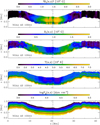 |
Fig. 8. Same as Fig. 7 but for the sunspot NOAA AR 10944 (right-hand panel in Fig. 1). |
| In the text | |
|
Fig. 9. Maps of the geometrical height at which different τc levels are reached in NOAA AR 10923: τc = 1 (top left), τc = 10−1 (top right), τc = 10−2 (bottom left), and τc = 10−3 (bottom right). All values are given with respect to the geometrical height for that τc level in the quiet Sun, zqs(τc). The quiet-Sun value is calculated as the spatial average over the white rectangle. |
| In the text | |
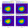 |
Fig. 10. Same as Fig. 9 but for NOAA AR 10944. |
| In the text | |
Current usage metrics show cumulative count of Article Views (full-text article views including HTML views, PDF and ePub downloads, according to the available data) and Abstracts Views on Vision4Press platform.
Data correspond to usage on the plateform after 2015. The current usage metrics is available 48-96 hours after online publication and is updated daily on week days.
Initial download of the metrics may take a while.