| Issue |
A&A
Volume 708, April 2026
|
|
|---|---|---|
| Article Number | A351 | |
| Number of page(s) | 14 | |
| Section | The Sun and the Heliosphere | |
| DOI | https://doi.org/10.1051/0004-6361/202659286 | |
| Published online | 27 April 2026 | |
Chromospheric and photospheric properties of sunspots as inferred from Stokes inversions under magnetohydrostatic and non-local thermodynamic equilibrium
1
Institut für Sonnenphysik, Georges-Köhler-Allee 401A, 79110 Freiburg, Germany
2
Institute for Solar Physics, Department of Astronomy, Stockholm University, AlbaNova University center, 10691 Stockholm, Sweden
3
Leibniz-Institut für Astrophysik Potsdam (AIP), An der Sternwarte 16, 14482 Potsdam, Germany
4
ETH Zürich, Institute for Particle Physics and Astrophysics, Wolfgang-Pauli-Strasse 27, 8093 Zürich, Switzerland
5
Istituto ricerche solari Aldo e Cele Daccò (IRSOL), Faculty of Informatics, Università della Svizzera italiana, CH-6605 Locarno, Switzerland
★ Corresponding author: This email address is being protected from spambots. You need JavaScript enabled to view it.
Received:
2
February
2026
Accepted:
9
March
2026
Abstract
Context. Sunspots represent a key feature in the solar atmosphere to explore how magnetic fields interact with plasma flows, exhibiting large variations in physical parameters over very small spatial scales (< 100 km), and sometimes featuring dynamic phenomena such as oscillatory umbral flashes. To fully understand the thermodynamic, magnetic and kinematic structure of these regions, from the stable photosphere to the shock-dominated chromosphere, Stokes inversion techniques are employed to jointly model these layers.
Aims. We aim to determine the average thermal, magnetic, and kinematic properties of a sunspot from the photosphere to the chromosphere and to deepen our understanding of the properties of umbral flashes.
Methods. We analysed high-resolution spectropolarimetric data acquired with the CRISP instrument at the Swedish Solar Telescope (SST). The dataset includes full Stokes measurements of the Mg I 517.2 nm, Na I 589.5 nm, Fe I 630.2 nm, and Ca II 854.2 nm spectral lines. We performed inversions using the FIRTEZ code, which includes non-local thermodynamic equilibrium (NLTE) and 3D magnetohydrostatic (MHS) equilibrium to constrain the gas pressure and density.
Results. We successfully inferred the physical parameters in a three-dimensional (x, y, z) domain and provide their average values as a function of the radial distance from the sunspot’s center at different heights. Among other findings, we determine that the photospheric Evershed flow is found to reverse into the inverse Evershed inflow in the upper photosphere. In contrast, the moat flow outside the sunspot persists as an outflow at similar heights, suggesting that it is not a direct continuation of the Evershed flow. Furthermore, analysis of an umbral flash event reveals supersonic upflows (Mach numbers ∥M∥≥1.5) and thermodynamic conditions consistent with shock fronts.
Conclusions. The application of 3D MHS equilibrium and NLTE effects combined with multiple lines sensing different layers of the atmosphere allows for the reliable retrieval of atmospheric parameters, which are typically difficult to simultaneously constrain in the photosphere and chromosphere. The inferred properties of umbral flash show clear evidence of shock dynamics, coinciding with previous theoretical and observational studies that point to converging supersonic flows that move the optical depth iso-surfaces as the driving mechanism behind umbral flashes.
Key words: Sun: activity / Sun: chromosphere / Sun: magnetic fields / Sun: photosphere
© The Authors 2026
 Open Access article, published by EDP Sciences, under the terms of the Creative Commons Attribution License (https://creativecommons.org/licenses/by/4.0), which permits unrestricted use, distribution, and reproduction in any medium, provided the original work is properly cited.
This article is published in open access under the Subscribe to Open model. This email address is being protected from spambots. You need JavaScript enabled to view it. to support open access publication.
1. Introduction
Sunspots are the most visible manifestation of the solar magnetic field. Their existence has been known for thousands of years, from naked-eye observations in ancient China and routine telescopic observations of sunspots recorded for hundreds of years by Harriot, Fabricius, Scheiner, Galileo and others (Vaquero & Vázquez 2009), to modern telescopes capable of recording sunspots’ polarized spectra with high spatial, spectral, and temporal resolution. Thanks to advanced analysis techniques such as spectropolarimetry, our knowledge of sunspots has advanced significantly (Solanki 2003; Borrero & Ichimoto 2011; Rempel & Borrero 2021).
Unfortunately, this knowledge pertains mainly to the deepest layers of the solar atmosphere, known as the photosphere (Lites et al. 1993; Stanchfield et al. 1997; Martinez Pillet 1997; Mathew et al. 2003). Higher layers such as the chromosphere have traditionally been more difficult to study due to deviations from hydrostatic and local thermodynamic equilibrium (LTE) that hinder the analysis of the spectra and their polarization signals. Over the past couple of decades the analysis techniques have matured to a point where non-LTE (NLTE) effects (Socas-Navarro et al. 2015; de la Cruz Rodríguez et al. 2019) and magnetohydrostatic (MHS) equilibrium (Borrero et al. 2021) can be routinely accounted for, making it possible to study the chromosphere of sunspots (Socas-Navarro 2005; de la Cruz Rodríguez et al. 2013). Despite these important advances, a comprehensive study of the magnetic, kinematic, and thermal properties of sunspots in the chromosphere is still lacking. This knowledge can have important applications in a number of fields. It can be used to constrain the upper boundary conditions of 3D magnetohydrodynamic (MHD) simulations of sunspots (Rempel 2012; Jurčák et al. 2020), or as a background model where the propagation of MHD waves from the photosphere into the chromosphere and their role in heating the upper atmospheric layers can be studied (Khomenko & Collados 2008; Felipe 2012; Felipe et al. 2014). In addition, it can be used to improve the determination of center-to-limb curves used in the study of stellar activity cycles and exoplanet detection and characterization (Lim et al. 2023; Sumida et al. 2026; Nèmec et al. 2026; Cauley et al. 2018; De Wilde et al. 2025).
In the present paper, we employ spectropolarimetric observations of several photospheric and chromospheric spectral lines in a sunspot to determine its average physical properties (e.g. temperature, gas pressure, Wilson depression, magnetic field, line-of-sight velocity) as a function of the radial distance from the sunspot’s center and at various optical depths, ranging from the photosphere to the mid-chromosphere. This is done via the application of a novel Stokes inversion technique (Pastor Yabar et al. 2019) that simultaneously accounts for NLTE effects (Kaithakkal et al. 2023; Borrero et al. 2024a) and for the effect of the Lorentz force (i.e. MHS equilibrium) in the thermodynamic structure of the sunspot. In addition to this, we present the results inferred from this inversion technique of a region of the sunspot umbra characterized by the presence of an umbral flash.
2. Observations
The data analysed in this work were recorded with the CRisp Imaging SpectroPolarimeter (CRISP) instrument (Scharmer et al. 2008) attached to the 1-metre Swedish Solar Telescope (SST). CRISP was used to measure the Stokes parameters I = (I, Q, U, V) across several photospheric and chromospheric spectral lines: Mg I 517.2 nm (also known as Fraunhofer’s Mg b2 line), Na I 589.5 nm (Fraunhofer’s Na D1 line), Fe I 630.2 nm, and Ca II 854.2 nm. The atomic data of the recorded spectral lines are summarized in Table 1, while the observed wavelengths are given in Table 2.
Atomic parameters of the spectral lines analysed in this work.
Scanning positions of the observed spectral lines.
The observation strategy followed the one described in Morosin et al. (2020). The number of accumulations per wavelength and per modulation state was twenty for 854.2 nm and ten for the rest of the spectral windows, and the exposure time per accumulation is 12 milliseconds. Part of data processing consisted of image reconstruction using the multi-object multi-frame blind deconvolution technique (MOMFBD Löfdahl 2002; van Noort et al. 2005) to remove the effects of atmospheric seeing during data acquisition and reach diffraction-limited observations. Given that the diffraction limit varies with wavelength, the data were first co-aligned and de-stretched using wide-band data for each spectral window and taking as a reference the shortest wavelength (517.2 nm). The narrow-band data were first corrected for cavity errors (small wavelength shifts) and then downgraded to the largest spatial sampling (589.6 nm), where the pixel scale is 0.0446″ pix−1. The size of the observed field of view is about 59″ × 59″, sampled in a total of 1358 × 1321 pixels.
The noise level achieved in the polarization signals is estimated by calculating the standard deviation of the polarization profiles at a fixed wavelength position. The wavelength used was in our case −0.6 Å from the center of the Fe I line, where no signal should be present in Q, U and V. This yields a noise level of σpol ≈ 1.6 × 10⁻³. The data described here are referred to as diffraction-limited data.
In addition to the diffraction-limited data, in this work we also analyse spatially averaged data where the diffraction-limited data are binned in a 4 × 4 pixel region, resulting in a pixel scale of 0.176″ pix−1 and a total of 339 × 330 pixels on the solar surface (x, y). We estimate the noise level in the polarization signals of the binned data to be σpol ≈ 1.2 × 10⁻³. The noise reduction achieved by binning deviates from the expected scaling of  . This occurs because the noise in the diffraction-limited data is spatially correlated, a consequence of the Wiener filter applied during the MOMFBD image reconstruction, which amplifies low-frequency noise components while suppressing high-frequency power, thus resulting in a lower than expected noise reduction.
The target recorded with the CRISP instrument corresponds to NOAA AR 13433 and was observed on 15 September 2023 at 8:38 UT. At this time, the center of the sunspot was located at approximate coordinates (−458″, 355″) corresponding to a heliocentric angle Θ ≈ 39.4° (i.e., μ ≈ 0.77). Maps of the intensities observed at different wavelengths are shown in the top panels of Figure 2. The first one corresponds to the continuum intensity at 630 nm, whereas the second and third maps show the observed intensity at the line core position of the Mg I and Ca II lines, respectively. In this order, they are meant to represent three different layers of the solar atmosphere: the photospheric continuum, the upper photosphere, and the chromosphere sampled by these spectral lines (see also Appendix A). Figures 2 and 3 contain three blue concentric circles around the sunspot’s center (indicated by the red cross in the umbra). These circles are meant to approximately represent the umbra-penumbra boundary, penumbra-quiet Sun boundary, and superpenumbral boundary, respectively. They are located around r/Rs = 0.3, 1.0 and 1.4, respectively, where Rs represents the sunspot’s radius. In our case Rs = 22″.
3. Stokes inversion and results
3.1. Inversion procedure
The Stokes inversion code used in this work is the FIRTEZ code (Pastor Yabar et al. 2019; Borrero et al. 2019). This code derives the physical parameters in the 3D domain (x, y, z), representing the solar atmosphere, from observations of the Stokes measurements on the solar surface I(x, y, λ). The simultaneous inversion of multiple spectral lines that form under potentially different physical conditions, such as local versus non-local thermodynamic equilibrium (LTE vs. NLTE), and at different heights, while enforcing physical constraints like MHS equilibrium, is a delicate task that deserves special attention.
Although the general procedure has been described in detail in Borrero et al. (2024a), here we provide a brief summary and some additional details when the approach deviates from the one described in the aforementioned paper. In this context, it is important to mention that for this work, the NLTE treatment in FIRTEZ has been improved by separating the source function into its contributions: one arising from the continuum and another contribution arising from the atomic transition (i.e. spectral line), with only the latter being affected by the departure coefficients. These modifications are detailed in Appendix B.
To initialize the inversion, we first obtained a guess of the physical parameters. To this end, we used the temperature and gas pressure from the VALC model (Vernazza et al. 1981) interpolated to 128 vertical grid points with a spacing of Δz = 12 km (Δlog τc ≈ 10−1 in the deep photosphere). The initial estimates for the magnetic field and line-of-sight velocity were done using simple estimations via the weak field approximation and the center of gravity method, respectively, and derived from the Fe I line at 630 nm only. Consequently, the initial estimate for these two parameters had constant values with optical depth. The VALC model was also used to compute initial departure coefficients for the Mg I, Na I, and Ca II spectral lines (see Figure C.1). More information on the determination of the departure coefficients can be found in Appendix C. The Fe I line at 630 nm was always considered to be formed under LTE conditions. The inversion procedure was divided into several inversion cycles. During each inversion cycle, the departure coefficients are kept constant. This approach is similar to the so-called fixed departure coefficient approximation (FDC; Socas-Navarro et al. 1998). All inversion cycles described hereafter were carried out by giving equal weights to the four Stokes parameters (I, Q, U, V).
With these ingredients, a first inversion cycle of the spatially binned data (see the description in Sect. 2) was performed employing vertical (i.e. one-dimensional) hydrostatic equilibrium. Four nodes were used for each of the following physical parameters: temperature T, line-of-sight velocity vlos, micro-turbulent velocity vmic, and the three components of the magnetic field (Bx, By, Bz). This represents a total of 24 free parameters that were used to fit a total of 232 observed wavelengths (Nλ,obs = 58 for each of the four Stokes parameters; see Table 2).
After the first inversion cycle, the resulting components of the magnetic field perpendicular to the line-of-sight (Bx, By) were then corrected from the 180° ambiguity using the non-potential field calculation method (Georgoulis 2005). Next, the gas pressure is recalculated under the assumption of 3D MHS (i.e., taking into account the Lorentz force) as described in Borrero et al. (2021). Because the temperature and gas pressure had changed through the application of the Stokes inversion and MHS equilibrium, some of the departure coefficients (obtained for a VALC model) were no longer representative of the new physical conditions. Therefore, in principle they should have been recalculated for every point on the 3D domain and for each spectral line formed under NLTE conditions. In practice, however, this was done only for the Ca II line, with the departure coefficients for Mg I and Na I being kept the same as determined initially for the VALC model. This decision is justified in detail in Appendix C. After this, the fit to the observed Stokes profiles was no longer adequate, and therefore a new inversion cycle of the spatially binned data was performed (keeping the gas pressure constant to what the MHS equilibrium established) to make sure the new physical parameters adapted to the change in the departure coefficients. The number of nodes was now reduced to: three for T, vlos and vmic, and two for Bx, By, and Bz (15 in total).
After the second inversion cycle, we obtained the temperature T(x, y, z), line-of-sight velocity vlos(x, y, z), magnetic field B(x, y, z), gas pressure Pg, and density ρ(x, y, z). We emphasize that because FIRTEZ determines the gas pressure using the 3D MHS equilibrium instead of the vertical hydrostatic equilibrium, the physical parameters were inferred in the (x, y, z) domain in addition to the more commonly used (x, y, τc), where τc refers to the optical depth (Borrero et al. 2021). The conversion between z and τc is non-linear and therefore surfaces of constant optical depth do not correspond to surfaces of constant z, as can be seen in panel f of Fig. 4 and on the vertical cut of Fig. 5.
At this point, we recall that the procedure described above applies to the inversion of the spatially binned data (see Section 2). The inversion of the diffraction-limited data was done by reinterpolating the results of the inversion of the binned data (330 × 330 pixels) to the original resolution (1321 × 1358 pixels) and using this as an initial guess in a new inversion cycle that fitted the diffraction-limited data. This new inversion was performed with the same number of nodes or free parameters as in the second cycle of the inversion of spatially binned data: three for T, vlos and vmic and two for Bx, By and Bz. The reason for doing this was twofold. First, it helped save computation time, as the initial inversion steps, MHS determination of the gas pressure, and recalculation of departure coefficients were done at a lower resolution (i.e. a lower number of spatial pixels). Second, the lower noise level in the spatially binned data helped obtain smoother maps that were then used to initialize the inversion of the diffraction limited data. This significantly improved the results for the components of the magnetic field perpendicular to the observer’s line-of-sight (Bx, By) that were inferred from the typically low signals in the linear polarization Stokes Q and U. This also improved the subsequent 180° disambiguation and therefore also the determination of the Lorentz force and gas pressure via MHS equilibrium. Examples of representative line profiles of the observations along with their fitted profiles for the diffraction limited data are shown in Fig. 1.
 |
Fig. 1. Representative Stokes profiles at three different locations in the diffraction limited observations. The three locations are: penumbra (green), umbra (blue), umbral flash (red). The points display the observed data whereas solid lines correspond to the fitted profiles. The profiles are normalized to the quiet sun continuum and to better visualize the data, vertical shifts have been applied. These are: [ + 0.2, 0, −0.2] in Stokes I and [ + 0.02, 0, −0.02] in Stokes Q, U and V. In addition, Stokes I signals in the umbra (blue) and umbral flash (red) have been multiplied by a factor of 2 before the shift is applied to better display the variations. |
3.2. Inversion results
As a result of the Stokes inversion described in Sect. 3.1 the FIRTEZ code provides the following physical parameters: temperature T, magnetic field vector B, line-of-sight velocity vlos, micro-turbulent velocity vmic, gas pressure Pg, density ρ, and continuum optical depth τc with its corresponding uncertainties. The uncertainties were computed using the inverse of the Hessian matrix (see Eq. (4) in Borrero et al. 2024b). Although this method can differ from the true error of the complete inversion process (i.e, it neglects degeneracies and local minima), over or underestimating: the true error depending on the relative strength of the neglected effects, it is sufficient to give us a proxy of how narrow is the χ2 valley in the inversion process.
All physical parameters are provided in a (x, y, z) 3D domain that is a combination of the (x, y) domain from the observed Stokes parameters (see Sect. 2) and the z domain from the initial 1D guess model (VALC; see Sect. 3.1). Consequently, the inversion of spatially binned data in the 3D domain has nx = 339, ny = 330, nz = 128 points, with the following spacing along each of those dimensions: Δx = Δy = 176 km, Δz = 12 km. On the other hand, the 3D domain in the inversion of diffraction limited data has nx = 1358, ny = 1321, nz = 128 points with spacings of Δx = Δy = 44 km, Δz = 12 km. To illustrate how the vertical height z maps to the more commonly used optical depth τc scale, we show some hints at panel f of Fig. 4 and in the vertical cut of Fig. 5. In the remaining of this section and in Section 4 the results from the inversion of the spatially binned data will be used. Section 5 employs the results of the inversion of the diffraction limited data.
3.2.1. Temperature
Figure 2 (middle row panels) shows the inferred temperature T as a function of (x, y) for three different surfaces of constant optical depth: τc = 1 (i.e. deep photosphere), τc = 10−2.5 (i.e. high photosphere), and τc = 10−5 (chromosphere). As demonstrated in Appendix A, our observed spectral lines provide us with reliable information in all these regions. As can be seen, the temperature maps in the middle panels of Fig. 2 display a very high correlation with the observed intensity levels at the three different wavelengths presented in the upper panels of the same figure.
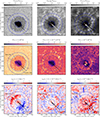 |
Fig. 2. Observations and inversion results. Top panels: Maps of the observed intensity at three different wavelengths (from left to right): continuum of the Fe I line at 630 nm, core of the Mg I line at 517 nm, and core of the Ca II line at 854 nm. Middle panels: Temperature inferred from the inversion at three different optical depth levels (from left to right): τc = 1 (photospheric continuum), τc = 10−2.5 (high photosphere), and τc = 10−5 (chromosphere). Bottom panels: Same as middle panels but showing the inferred line-of-sight velocity. Inner and outer blue circles are located at radii r/Rs = 0.4, 1.0, 1.4, respectively, where Rs is defined as the sunspot’s radius as measured from the umbral center (red cross). The direction of the solar disk center is indicated by the bold arrow. Dashed black lines depict a cone of ±15° around the line of symmetry of the spot. |
3.2.2. Line-of-sight velocity
Velocities in the deep photosphere (τc = 1; bottom-left panel in Fig. 2) show the common pattern characterized by vlos < 0 (i.e. velocities towards the observer) in the penumbral region facing the center of the solar disk, and vlos > 0 (i.e. velocities away from the observer) in the penumbral region facing the solar limb. This is seen not only in the penumbra, r/Rs ∈ [0.4, 1.0], but also beyond the limit of the sunspot’s outer boundary, r/Rs > 1. While within the sunspot this corresponds to the well known Evershed outflow (Evershed 1909), outside it is indicative of the so-called moat outflow (Pardon et al. 1979; Nye et al. 1988). In the upper photosphere (τc = 10−2.5; bottom-middle panel) the velocity pattern within the penumbra already switches to the inverse Evershed effect (i.e. inflow towards the sunspot’s center). This supports previous works in wich the inverse Evershed flow appear not only as a purely chromospheric phenomenon but is already visible in the photosphere (Deming et al. 1988; Borrero et al. 2008). The exact optical depth at which the Evershed flow turns into the inverse Evershed flow appears to be somewhere between τc ∈ [10−2, 10−3] (see also Section 4).
Interestingly, while the penumbral Evershed flow reverses into an inflow in the upper photosphere (τc = 10−3), beyond the visible limit of the spot (r/Rs) the moat flow continues as an outflow at similar heights. These results suggest that the moat flow is not the continuation of the Evershed flow (Löhner-Böttcher & Schlichenmaier 2013), otherwise the moat flow should also have reversed (Vargas Domínguez et al. 2007, cf.).
In the chromosphere (τc = 10−5; bottom-right panel), the inverse Evershed effect completely takes over not only in the penumbra, but also in the moat immediately outside the sunspot. The velocity pattern closely resembles what is usually identified as superpenumbral fibrils. The fact that the moat outflow has now dissipated could be interpreted as the moat outflow being confined to underneath the sunspot’s magnetic canopy.
In the quiet Sun surrounding the sunspot and beyond the moat r/Rs > 1.4 there is a pattern of upflows and downflows at τc = 1 (bottom-left panel in Fig. 2) that does not entirely resemble the well-known convective pattern of bright or dark structures that are correlated with up or downflows. This happens because our observations are located far from the disk center (see Sect. 2) and, therefore, granular and/or intergranular intensity patterns and the inferred line-of-sight velocities appear distorted. This is evidenced by the fact that the line-of-sight velocities in the quiet Sun show clear structuring on the (x, y) plane along the direction perpendicular to the line-of-sight (thick arrow in Fig. 2). However, the convective pattern is not entirely lost. In fact, the correlation between the observed continuum intensity (upper-left panel) and the inferred vlos(τc = 1) (bottom-left panel) is −0.23, lower than the typical values of −0.6 at disk center, but still negative, meaning that bright structures show preferentially upflows, whereas dark structures tend to harbour downflows.
3.2.3. Magnetic field vector
Stokes inversion codes, such as FIRTEZ, provide the magnetic field vector B in a reference frame where the z-axis is aligned with the observer’s line-of-sight. This is the so-called observer’s reference frame. However, since FIRTEZ corrects the 180°-ambiguity of the magnetic field in the plane perpendicular to the observer, it is possible to express the magnetic field vector B in a new reference frame where the x and y axes are parallel to the equatorial and meridional lines and where the z-axis is perpendicular to the solar surface (Gary & Hagyard 1990). This is referred to as the local reference frame.
Figure 3 presents the maps of these three components of the magnetic field in the local reference frame at three different heights in the solar atmosphere. Owing to the weak observed polarization signals in the Na I, Mg I and Ca II lines in the quiet Sun, the magnetic field inferred from the inversion in this region is particularly unreliable. There large values of Bx, By seen at τc = 10−5 (i.e., chromosphere) in the quiet region around the sunspot are a clear example. A more detailed description of the errors of the inversion in the observer’s reference frame is provided in Table 3. We note that in the local reference frame, the horizontal and vertical errors have to be computed through error propagation, and therefore will probably lie between the ones shown for Bz and Bhor. Because of this, we do not discuss the magnetic field inferred in this region.
 |
Fig. 3. Inversion results. Similar to middle and bottom panels of Fig. 2 but displaying the Bx (top), By (middle) and Bz (bottom) components of the magnetic field in the local reference frame at three different optical depths. |
Mean inversion errors in 10 × 10 pixel regions.
Within the sunspot, Fig. 3 shows that the component of the magnetic field perpendicular to the solar surface Bz is largest at the sunspot’s center, while Bx and By are largest in the penumbra. In all three cases, the magnetic field components decrease with height, that is, Bx, By and Bz are larger in the low photosphere (τc = 1) than in the high photosphere and chromosphere (τc = 10−2.5, 10−5, respectively).
4. Azimuthal averaged sunspot properties
In this section, we present the azimuthal averaged physical properties of the observed sunspot as a function of the normalized radial distance from the sunspot’s center at different optical depth levels (r/Rs, log τc). We note that the very center of the umbra is avoided (r/Rs ≥ 0.05) because at short radial distances we have very few points to average over. Results are presented in Fig. 4 and include: module of the magnetic field vector (∥B∥; panel-a), vertical component of the magnetic field in the local reference frame (Bz; panel-b), horizontal component of the magnetic field in the local reference frame (Bh; panel-c), inclination of the magnetic field with respect to the direction normal to the solar surface (γ; panel-d), temperature (T; panel-e), Wilson depression (z; panel-f), gas pressure (Pg; panel-g), line-of-sight velocity in the center side of the penumbra (vlos; panel-h), and line-of-sight velocity in the limb side of the penumbra (vlos; panel-i). We note that since high spatial resolution is not needed in order to perform spatial averages, we do not use the results of the Stokes inversion of the diffraction limited data, but rather the results of the inversion of the spatially binned data (see Sect. 2).
 |
Fig. 4. Average sunspot properties. Azimuthal averages of the physical parameters, as inferred from the Stokes inversion, as a function of the normalized sunspot radius r/Rs at different optical-depth levels: log τc = 0 (red), −1 (orange), −2 (yellow), −3 (green), −4 (blue), −5 (cyan), −6 (purple). Typical deviations around the mean are represented by the vertical colour bars. All panels, except (h) and (i) were produced by averaging over 2π radians. Panels h (vlos in the center side penumbra) and i (vlos in the limb side penumbra) were obtained by averaging only over ±π/12 radians around the sunspot’s line of symmetry (see cone denoted by dashed lines in Figs. 2 and 3). |
With the exception of vlos, all azimuthal averages are performed over 2π angles around concentric circles to increase radial distances around the sunspot’s center (see examples of blue circles in Figs. 2 and 3). In the case of the line-of-sight velocity we do not perform 2π averages because, due to the photospheric Evershed flow redshifted velocities on the limb side of the penumbra will cancel with blueshifted velocities on the center side (see lower panels in Fig. 2). Likewise, due to the inverse Evershed flow in the chromosphere, redshifted velocities in the center side of the penumbra will cancel with blueshifted velocities on the center side. Instead of this, the averaged line-of-sight velocities are calculated in a cone of ±15° around the line of symmetry of the sunspot (see dashed lines in Figs. 2 and 3).
In addition to the mean values of the physical parameters as a function of (r/Rs, log τc) we also display, as vertical bars in Fig. 4, typical standard deviations of these physical parameters at different optical depths. We note that these bars do not represent errors in the inversion, but rather standard deviations around the mean value. In this regard, it is important to note that parameters such as ∥B∥, Bz, Bh and γ (panels a,b,c and d, respectively) feature a large deviation around the mean because of the presence of the penumbral fine structure, where regions of strong and vertical magnetic field (i.e. spines) are interlaced azimuthally with regions of much weaker and horizontal magnetic field (i.e. intraspines; Borrero et al. 2004, 2025).
The results presented in Fig. 4 are unique and expand on previous works (Title et al. 1993; Westendorp Plaza et al. 2001; Mathew et al. 2003; Bellot Rubio et al. 2004; Sánchez Cuberes et al. 2005; Borrero & Ichimoto 2011) in that we extend our analysis to part of the moat (r/Rs = 1.4) and to the temperature minimum and lower chromosphere (log τc ∈ [ − 4, −6]). Moreover, because our inversions were carried out using a 3D MHS equilibrium instead of vertical hydrostatic equilibrium (see Sect. 3.1) we can provide more reliable values for the gas pressure and Wilson depression (see panels h and g in Fig. 4) than those reported in previous works. On the basis of the various panels in this figure, we can make a number of additional observations.
-
In the umbra and mid-inner penumbra (r/Rs < 0.6) we find that dB/dτc > 0, whereas in the outer penumbra (r/Rs ≥ 0.6) this derivative changes sign: dB/dτc < 0. This is reminiscent of previous findings by Borrero & Solanki (2008, see their Fig. 4) even though that work focused primarly on the penumbral intraspines, whereas here we have averaged azimuthally over both spines and intraspines.
-
In the moat and superpenumbra (r/Rs ≥ 1.0) the trend dB/dτc < 0 continues. Moreover, the radial component of the magnetic field Bh (panel c) in the moat and superpenumbra is larger in the chromosphere than in the photosphere. Although it might be tempting to interpret this result in terms of the presence of a magnetic canopy, we refrain ourselves from such an interpretation as we have already established that the inference of the magnetic field outside the spot at chromospheric heights is not reliable due to the low polarization signals observed in the Ca II spectral line.
-
Physical parameters such as temperature (panel e), Wilson depression (panel f), and line-of-sight velocity on the center side of the penumbra (panel h) feature large variations (seen sometimes as dips, sometimes as peaks) very close to the umbral center (r/Rs ≈ 0.1). These are produced by the presence of an umbral flash very close to the umbral center. This particular event will be studied in detail in Sect. 5.
-
On average the Wilson depression, z(τc = 1), is about 250 km deeper inside the umbra than in the quiet Sun (see panel f). Although this might be seen as too shallow, we emphasize that the highest value of the Wilson depression occurs in the very umbral center (which was avoided in these figures) and amounts to about 350 km.
-
The current values of the gas pressure Pg at different optical depth levels (panel g) look rather constant with the radial distance. This is an effect of having used iso-surfaces of optical depth. At fixed geometrical heights z the gas pressure would show much stronger variations with radial distance.
-
According to panels h and i, in the penumbra r/Rs ∈ [0.4, 1.0], the regular Evershed flow is still seen at optical depths τc = 10−2 (see yellow lines), whereas for optical depths τc = 10−3 (green lines) we already detect the inverse Evershed flow.
5. Instantaneous view of an umbral flash
As already mentioned in Sect. 4, an important aspect to notice in this particular dataset is the presence of an umbral flash or small-scale umbral brightening. Umbral flashes are known to be transient events that occur with a periodicity of about 3 minutes (Socas-Navarro et al. 2000) and unfortunately the analyzed data can only provide a picture of this phenomenon at a single instant in time. The umbral flash in our data occurs very close to the umbral center at (x, y)≈(−458″, 352″). In the spatially averaged data (Fig. 2) there is a sudden temperature enhancement at this location in the high photosphere (τc = 10−2.5). The enhancement spreads over a larger horizontal area at τc = 10−5 (i.e. chromosphere). These temperature enhancements are produced by the presence of the aforementioned umbral flash (Beckers & Tallant 1969; Wittmann 1969). Remarkably, while the core of the Ca II spectral line responds by increasing its intensity (see the upper-right panel in Fig. 2) and turning into emission (see the red lines in Fig. 1), the core of the Mg I line does not show any increase in the observed intensity (see the upper-middle panel in Fig. 2) in response to the aforementioned temperature increase. The core of the Na I line behaves similarly to the core of Mg I and displays no intensity enhancement (not shown). The reason for this different behaviour is provided in Appendix C, where we show that the Na I and Mg I lines strongly decouple from the local temperature in the upper photosphere and chromosphere, whereas the Ca II line stays more strongly coupled to the temperature.
In order to study the umbral flash in more detail we turn to the results of the inversion of the diffraction limited data (see Sect. 2). The Results of temperature T(x, y) and line-of-sight velocity vlos(x, y) at a constant geometrical height of z = 1.08 Mm, obtained from the Stokes inversion of the diffraction limited data, are presented in Fig. 5 (upper panel). This figure also displays, in the bottom panels, the temperature T, line-of-sight velocity normalized to the local sound speed or Mach number M = vlos/cs, and magnetic field B(y, z) in a (x, z) plane for a y value that cuts horizontally through the umbral flash (see dashed line). The local sound speed has been calculated assuming an adiabatic constant of γ = 5/3 (i.e. monoatomic gas).
 |
Fig. 5. View of the umbral flash inferred from the diffraction limited data. Upper panel: Divided map of temperature T(x, y) (bottom left) and line-of-sight velocity vlos (top right) at z ∼ 1 Mm. The horizontal dotted line represents the slice selected for the three lower panels, and the cross indicates where the umbral flash happens (i.e. where the strongest supersonic velocities are found). Bottom panels: Temperature T(x, z), Mach number M(x, z), and magnetic field B(x, z) on the plane of the slice indicated on the upper panel (y = 88 Mm). As a reference, the curves of constant optical depth log τc = 0, −2, −3, −4, −5 are indicated by the dashed black or white lines. Green contours indicate the regions where supersonic flows are found: ∥M > 1∥. |
At the location of the umbral flash and its surroundings, there is a region where large temperature enhancements are found in the upper photosphere and chromosphere (τc ∈ [10−3, 10−6]). At these locations supersonic upflow velocities (M < −1) are also detected. These regions are marked within green contours, in the third row panel in Fig. 5. The magnetic field displayed in the lowest panel is converted to the local reference frame and displays typical sunspot behaviour. Here the flux tube is mostly vertical in the center (of around ∼5000 G) and opens towards the penumbra, becoming more horizontal. The umbral flash regions show disturbances in both strength (Δ|B|∼1 KG) and direction, mostly changing the horizontal components. Magnetic field variations show weakening and enhancements, consistent with Henriques et al. (2017). Values as high as ∥M∥≥1.5 are sometimes inferred. We note that the previous inequalities on the supersonic velocities are because they are computed from the line-of-sight component of the velocity alone, and therefore, even larger values are to be expected if we consider the full velocity vector. Unfortunately, measurements of the components of the velocity vector in the plane perpendicular to the line-of-sight are usually not possible (cf. Vila Crespo et al. 2026). The existence of these supersonic velocities bespeaks the presence of a shock front (de la Cruz Rodríguez et al. 2013). In agreement with previous studies (Henriques et al. 2017; Bose et al. 2019; Henriques et al. 2020) we also find that supersonic upflows are surrounded by large, albeit still subsonic, downflow velocities. Henriques et al. (2020) [see Sect. 4.2] have argued that there is an intrinsic degeneracy in the inference of the temperature in umbral flashes by Stokes inversion codes. This degeneracy arises because an increase in the source function needed to produce emission in the line core of the Ca II line (see the red lines in the upper panel of Fig. 1) can be caused by either an increase in the density or an increase in the temperature. Now, because Stokes inversion codes have traditionally operated under the assumption of vertical hydrostatic equilibrium, they cannot produce local enhancements in density. This is not the case for the FIRTEZ inversion code, where 3D MHS equilibrium can produce those local enhancements through the action of the Lorentz force. We note that this is the first time such studies have been carried out, and therefore we can better constrain the origin of the source function enhancement in the umbral flash region.
However, according to Henriques et al. (2020), the reason density enhancements occur is due to the presence of converging flows, and these are not accounted for in FIRTEZ. To do so, FIRTEZ would have to determine the density and gas pressure not under MHS conditions but rather under magnetohydrostationary conditions (i.e. including the advective velocity term, ρ(v ⋅ ∇)v, in the momentum equation). Adding this term would be particularly beneficial in the case of umbral flashes due to the presence of supersonic velocities.
Figure 6 shows the thermodynamic (temperature T, gas pressure Pg, and density ρ) as well as kinematic (Mach number M) parameters present in one pixel where the aforementioned shocks are detected. These physical parameters are displayed as a function of the geometric height z (blue lines), and as a function of the logarithm of the continuum optical depth log τc (red lines). As can be seen, there are clear supersonic velocities and temperature enhancements in the upper photosphere and chromosphere: log τc < −2.5. It is worth noting that the consideration of the supersonic regime of some inverted pixels already takes into account the uncertainties of the inversion process as described in Sect. 3.2. Similar results to those shown in Fig. 6 also appear in several pixels around the umbral flash. Temperature errors, although also included in this figure (top panel), are below the line width (20 < δT < 100 K).
 |
Fig. 6. Atmosphere stratification of one of the pixels of the umbral flash with supersonic velocities. From top to bottom: Temperature T, line-of-sight velocity normalized to the local sound speed (i.e. line-of-sight Mach number) vlos/cs, logarithm of density log ρ, and logarithm of gas pressure log Pg. Bottom axis and red lines represent the physical parameters as a function of the optical depth scale log τc, whereas the upper axis and blue lines represent the physical parameters as a function of geometrical height z. We note the continuum (log τc = 0) is formed at around z ≈ 0.2 Mm above the lowermost boundary of the domain. Error estimations inferred from the Stokes inversion are presented for the temperature and velocity as shadowed areas. The horizontal dashed line represents the limit at which the line-of-sight velocity becomes supersonic. |
Comparison of both vertical scales, z and log τc, in combination with optical depth surfaces (shown as dashed coloured lines in Fig. 5) suggests that the opacity increases greatly at the top of the atmosphere, where the temperature enhancement is located, and then drops significantly below until the optical depth matches with the surrounding columns around log τc ∼ −2.5. This phenomenon compresses the tau scale in z at the higher layers, removing the sensitivity on the τ scale between the heights of the and the base of the umbral region.
6. Conclusions
In this paper we analysed spectropolarimetric data of a sunspot that included multiple spectral lines formed in the photosphere and chromosphere. The spectral lines were recorded with the CRISP instrument (Scharmer et al. 2008) attached to the 1-m SST Telescope. The analysis was performed with the FIRTEZ Stokes inversion code (Pastor Yabar et al. 2019) which provides us with the sunspot’s kinematic, thermodynamic and magnetic properties.
Owing to NLTE effects being included in the analysis, our inferences are valid from the deep photosphere to the mid chromosphere simultaneously, which makes it particularly interesting. This corresponds to a height range that spans up to six orders of magnitude of optical depth: log τc ∈ [0, −5]. In addition, the Stokes inversion accounted for MHS constraints and therefore inferences are also valid on the geometrical height scale (Borrero et al. 2021). In this case, the height range is where the physical parameters are z − z(τc = 1)∈[0, 1] Mm, where z(τc = 1) refers to the layer where the continuum is formed (see, e.g. dashed black line in the bottom panels of Fig. 5).
With these results we studied the average sunspot properties (such as temperature, line-of-sight velocity, magnetic field vector, gas pressure, Wilson depression) as a function of radial distance from the sunspot’s center and as a function of geometrical height and optical depth (r, z, τc). This work extends similar studies that mostly concern the photospheric properties (Mathew et al. 2003; Borrero & Ichimoto 2011) to include also the chromosphere and expand the analysis giving a tomographic view of the sunspot due to the coupling capabilities that FIRTEZ inversion code provides. We have also extended previous analysis to radial distances beyond the penumbra-quiet Sun boundary (r/Rs > 1) to include part of the moat and superpenumbra.
In addition, very close to the umbral center, an umbral flash is detected in our data. Although umbral flashes are characterized by oscillatory behaviour in time (Socas-Navarro et al. 2000; Henriques et al. 2020), the data we have analysed here only capture a single time instance and therefore cannot be used to fully describe these phenomena. However, at the particular time of our observations, the umbral flash appears in the upper photosphere and chromosphere (τc ∈ [10−3, 10−6]) where it manifests itself with large temperature and opacity enhancements. In addition, supersonic upflowing line-of-sight velocities vlos/cs ≈ −1.5 are seen at the center of the umbral flash. These are surrounded by large, subsonic, downflowing line-of-sight velocities vlos/cs ≈ 0.5. These results support the idea that umbral flashes are caused by converging flows that produce hydrodynamic shocks (Henriques et al. 2020). In the future we will try to analyse a time series of these observations and fully characterize the temporal behaviour of the umbral flash in the correct z-scale by means of the NLTE MHS Stokes inversion described in this paper.
Acknowledgments
The development of the FIRTEZ inversion code is funded by two grants from the Deutsche Forschung Gemeinschaft (DFG): projects 321818926 and 538773352. AVA acknowledges support from the DFG (project 538773352). APY acknowledges support from the Swedish Research Council (grant 2023-03313). This project has been funded by the European Union through the European Research Council (ERC) under the Horizon Europe program (MAGHEAT, grant agreement 101088184). AP was supported by grant PI 2102/1-1 from the Deutsche Forschungsgemeinschaft (DFG). IK was supported by the Deutsche Forschungsgemeinschaft (DFG) project number KO 6283/2-1. This research data leading to the results obtained has been supported by SOLARNET project that has received funding from the European Union’s Horizon 2020 research and innovation programme under grant agreement no 824135. This research has made use of NASA’s Astrophysics Data System and of the atomic data publicly provided by the National Institute of Standards and Technology (US Department of Commerce).
References
- Anstee, S. D., & O’Mara, B. J. 1995, MNRAS, 276, 859 [Google Scholar]
- Barklem, P. S., & O’Mara, B. J. 1997, MNRAS, 290, 102 [Google Scholar]
- Barklem, P. S., O’Mara, B. J., & Ross, J. E. 1998, MNRAS, 296, 1057 [Google Scholar]
- Beckers, J. M., & Tallant, P. E. 1969, Sol. Phys., 7, 351 [NASA ADS] [CrossRef] [Google Scholar]
- Bellot Rubio, L. R., Balthasar, H., & Collados, M. 2004, A&A, 427, 319 [NASA ADS] [CrossRef] [EDP Sciences] [Google Scholar]
- Borrero, J. M., & Ichimoto, K. 2011, Liv. Rev. Sol. Phys., 8, 4 [Google Scholar]
- Borrero, J. M., & Solanki, S. K. 2008, ApJ, 687, 668 [Google Scholar]
- Borrero, J. M., Solanki, S. K., Bellot Rubio, L. R., Lagg, A., & Mathew, S. K. 2004, A&A, 422, 1093 [NASA ADS] [CrossRef] [EDP Sciences] [Google Scholar]
- Borrero, J. M., Lites, B. W., & Solanki, S. K. 2008, A&A, 481, L13 [NASA ADS] [CrossRef] [EDP Sciences] [Google Scholar]
- Borrero, J. M., Pastor Yabar, A., Rempel, M., & Ruiz Cobo, B. 2019, A&A, 632, A111 [NASA ADS] [CrossRef] [EDP Sciences] [Google Scholar]
- Borrero, J. M., Pastor Yabar, A., & Ruiz Cobo, B. 2021, A&A, 647, A190 [NASA ADS] [CrossRef] [EDP Sciences] [Google Scholar]
- Borrero, J. M., Milić, I., Pastor Yabar, A., Kaithakkal, A. J., & de la Cruz Rodríguez, J. 2024a, A&A, 688, A56 [NASA ADS] [CrossRef] [EDP Sciences] [Google Scholar]
- Borrero, J. M., Pastor Yabar, A., & Ruiz Cobo, B. 2024b, A&A, 687, A155 [NASA ADS] [CrossRef] [EDP Sciences] [Google Scholar]
- Borrero, J. M., Pastor Yabar, A., Schmassmann, M., et al. 2025, A&A, 699, A149 [NASA ADS] [CrossRef] [EDP Sciences] [Google Scholar]
- Bose, S., Henriques, V. M. J., Rouppe van der Voort, L., & Pereira, T. M. D. 2019, A&A, 627, A46 [NASA ADS] [CrossRef] [EDP Sciences] [Google Scholar]
- Bruls, J. H. M. J., Rutten, R. J., & Shchukina, N. G. 1992, A&A, 265, 237 [NASA ADS] [Google Scholar]
- Cauley, P. W., Kuckein, C., Redfield, S., et al. 2018, AJ, 156, 189 [Google Scholar]
- de la Cruz Rodríguez, J., Socas-Navarro, H., Carlsson, M., & Leenaarts, J. 2012, A&A, 543, A34 [Google Scholar]
- de la Cruz Rodríguez, J., Rouppe van der Voort, L., Socas-Navarro, H., & van Noort, M. 2013, A&A, 556, A115 [NASA ADS] [CrossRef] [EDP Sciences] [Google Scholar]
- de la Cruz Rodríguez, J., Leenaarts, J., Danilovic, S., & Uitenbroek, H. 2019, A&A, 623, A74 [Google Scholar]
- De Wilde, M., Pietrow, A. G. M., Druett, M. K., et al. 2025, A&A, 700, A275 [NASA ADS] [CrossRef] [EDP Sciences] [Google Scholar]
- Deming, D., Boyle, R. J., Jennings, D. E., & Wiedemann, G. 1988, ApJ, 333, 978 [Google Scholar]
- Evershed, J. 1909, MNRAS, 69, 454 [Google Scholar]
- Felipe, T. 2012, ApJ, 758, 96 [Google Scholar]
- Felipe, T., Socas-Navarro, H., & Khomenko, E. 2014, ApJ, 795, 9 [NASA ADS] [CrossRef] [Google Scholar]
- Gary, G. A., & Hagyard, M. J. 1990, Sol. Phys., 126, 21 [Google Scholar]
- Georgoulis, M. K. 2005, ApJ, 629, L69 [Google Scholar]
- Henriques, V. M. J., Mathioudakis, M., Socas-Navarro, H., & de la Cruz Rodríguez, J. 2017, ApJ, 845, 102 [NASA ADS] [CrossRef] [Google Scholar]
- Henriques, V. M. J., Nelson, C. J., Rouppe van der Voort, L. H. M., & Mathioudakis, M. 2020, A&A, 642, A215 [NASA ADS] [CrossRef] [EDP Sciences] [Google Scholar]
- Hubeny, I., & Mihalas, D. 2015, Theory of Stellar Atmospheres. An Introduction to Astrophysical Non-equilibrium Quantitative Spectroscopic Analysis (Princeton series in Astrophysics) [Google Scholar]
- Jurčák, J., Schmassmann, M., Rempel, M., Bello González, N., & Schlichenmaier, R. 2020, A&A, 638, A28 [NASA ADS] [CrossRef] [EDP Sciences] [Google Scholar]
- Kaithakkal, A. J., Borrero, J. M., Pastor Yabar, A., & de la Cruz Rodríguez, J. 2023, MNRAS, 521, 3882 [NASA ADS] [CrossRef] [Google Scholar]
- Khomenko, E., & Collados, M. 2008, ApJ, 689, 1379 [NASA ADS] [CrossRef] [Google Scholar]
- Landi Degl’Innocenti, E. 1992, in Solar Observations: Techniques and Interpretation, eds. F. Sanchez, M. Collados, & M. Vazquez, 71 [Google Scholar]
- Leenaarts, J., Rutten, R. J., Reardon, K., Carlsson, M., & Hansteen, V. 2010, ApJ, 709, 1362 [NASA ADS] [CrossRef] [Google Scholar]
- Lim, O., Benneke, B., Doyon, R., et al. 2023, ApJ, 955, L22 [NASA ADS] [CrossRef] [Google Scholar]
- Lites, B. W., Elmore, D. F., Seagraves, P., & Skumanich, A. P. 1993, ApJ, 418, 928 [NASA ADS] [CrossRef] [Google Scholar]
- Löfdahl, M. G. 2002, SPIE Conf. Ser., 4792, 146 [Google Scholar]
- Löhner-Böttcher, J., & Schlichenmaier, R. 2013, A&A, 551, A105 [NASA ADS] [CrossRef] [EDP Sciences] [Google Scholar]
- Martinez Pillet, V. 1997, ASP Conf. Ser., 118, 212 [Google Scholar]
- Mathew, S. K., Lagg, A., Solanki, S. K., et al. 2003, A&A, 410, 695 [NASA ADS] [CrossRef] [EDP Sciences] [Google Scholar]
- Milić, I., & van Noort, M. 2018, A&A, 617, A24 [Google Scholar]
- Morosin, R., de la Cruz Rodríguez, J., Vissers, G. J. M., & Yadav, R. 2020, A&A, 642, A210 [NASA ADS] [CrossRef] [EDP Sciences] [Google Scholar]
- Nèmec, N.-E., Porqueras-León, Ò., Ribas, I., & Shapiro, A. I. 2026, A&A, 705, A111 [NASA ADS] [CrossRef] [EDP Sciences] [Google Scholar]
- Nye, A., Bruning, D., & Labonte, B. J. 1988, Sol. Phys., 115, 251 [NASA ADS] [CrossRef] [Google Scholar]
- Osborne, C. M. J., & Milić, I. 2021, ApJ, 917, 14 [NASA ADS] [CrossRef] [Google Scholar]
- Pardon, L., Worden, S. P., & Schneeberger, T. J. 1979, Sol. Phys., 63, 247 [Google Scholar]
- Pastor Yabar, A., Borrero, J. M., & Ruiz Cobo, B. 2019, A&A, 629, A24 [NASA ADS] [CrossRef] [EDP Sciences] [Google Scholar]
- Rempel, M. 2012, ApJ, 750, 62 [Google Scholar]
- Rempel, M., & Borrero, J. 2021, Oxford Research Encyclopedia of Physics [Google Scholar]
- Sánchez Cuberes, M., Puschmann, K. G., & Wiehr, E. 2005, A&A, 440, 345 [NASA ADS] [CrossRef] [EDP Sciences] [Google Scholar]
- Scharmer, G. B., Narayan, G., Hillberg, T., et al. 2008, ApJ, 689, L69 [Google Scholar]
- Shine, R. A., & Linsky, J. L. 1974, Sol. Phys., 39, 49 [NASA ADS] [CrossRef] [Google Scholar]
- Socas-Navarro, H. 2005, ApJ, 633, L57 [Google Scholar]
- Socas-Navarro, H., Ruiz Cobo, B., & Trujillo Bueno, J. 1998, ApJ, 507, 470 [NASA ADS] [CrossRef] [Google Scholar]
- Socas-Navarro, H., Trujillo Bueno, J., & Ruiz Cobo, B. 2000, Science, 288, 1396 [NASA ADS] [CrossRef] [Google Scholar]
- Socas-Navarro, H., de la Cruz Rodríguez, J., Asensio Ramos, A., Trujillo Bueno, J., & Ruiz Cobo, B. 2015, A&A, 577, A7 [NASA ADS] [CrossRef] [EDP Sciences] [Google Scholar]
- Solanki, S. K. 2003, A&ARv, 11, 153 [Google Scholar]
- Stanchfield, D. C. H., II., Thomas, J. H., & Lites, B. W. 1997, ApJ, 477, 485 [Google Scholar]
- Sumida, V. Y. D., Estrela, R., Swain, M., & Valio, A. 2026, A&A, 706, A281 [NASA ADS] [CrossRef] [EDP Sciences] [Google Scholar]
- Title, A. M., Frank, Z. A., Shine, R. A., et al. 1993, ApJ, 403, 780 [NASA ADS] [CrossRef] [Google Scholar]
- van Noort, M., Rouppe van der Voort, L., & Löfdahl, M. G. 2005, Sol. Phys., 228, 191 [Google Scholar]
- Vaquero, J. M., & Vázquez, M. 2009, The Sun Recorded Through History: Scientific Data Extracted from Historical Documents (New York, NY: Springer), 361 [Google Scholar]
- Vargas Domínguez, S., Bonet, J. A., Martínez Pillet, V., et al. 2007, ApJ, 660, L165 [NASA ADS] [CrossRef] [Google Scholar]
- Vernazza, J. E., Avrett, E. H., & Loeser, R. 1981, ApJS, 45, 635 [Google Scholar]
- Vila Crespo, H., Borrero, J. M., Milić’, M., Vigeesh, G., & Asensio Ramos, A. 2026, A&A, 707, A306 [NASA ADS] [CrossRef] [EDP Sciences] [Google Scholar]
- Vukadinović, D., Milić, I., & Atanacković, O. 2022, A&A, 664, A182 [NASA ADS] [CrossRef] [EDP Sciences] [Google Scholar]
- Westendorp Plaza, C., del Toro Iniesta, J. C., Ruiz Cobo, B., et al. 2001, ApJ, 547, 1130 [Google Scholar]
- Wittmann, A. 1969, Sol. Phys., 7, 366 [NASA ADS] [CrossRef] [Google Scholar]
Appendix A: Spectral lines and height sensitivity
In Figure A.1 we show spatially averaged response functions to several physical parameters for the observed spectral lines. They were calculated by averaging the absolute value of the response functions obtained from the atmospheric models as inferred from the Stokes inversion (see Section 3.1) in a region located in the penumbra and containing 10×10 pixels. All four Stokes parameters (I, Q, U, V) were used to calculate ℛℱT and ℛℱvlos but only Stokes V to determine ℛℱBz and only Q and U to calculate ℛℱBh. We note that the response functions are not evaluated with a constant Δlog τc-grid but rather in a constant Δz-grid. These plots illustrate that this combination of spectral lines provides a continuous height coverage ranging from the photospheric continuum (log τc = 0) until the mid chromosphere (log τc = −6). Note that the non-LTE lines (all the lines except the Fe I) quickly lose temperature sensitivity with height, due to the source function decoupling from the local temperature (see Appendix C). As explained there, this effect is actually more prominent in the Na I and Mg I lines than in the Ca II lines (see Fig. C.1). Meanwhile, the sensitivity to the magnetic field and velocity persists almost to log τc = −6. This is because this sensitivity comes predominantly from the line absorption/emission coefficient, which is a local quantity and is not affected by non-LTE effects.
 |
Fig. A.1. Response functions for the temperature (ℛℱT; upper-left), line-of-sight velocity (ℛℱvlos; upper-right), vertical component of the magnetic field (ℛℱBz; lower-left), and horizontal component of the magnetic field (ℛℱBh; lower-right) for a pixel located in the penumbra as a function of wavelength and optical depth log τc. See text for details. |
Appendix B: NLTE source functions
In previous works where the FIRTEZ inversion code was used to analyze spectral lines formed under non-LTE conditions (Kaithakkal et al. 2023; Borrero et al. 2024a), the total source total function S(λ, T) for such spectral lines was treated by FIRTEZ using the following expression:
![Mathematical equation: $$ \begin{aligned} S (\lambda ) = \frac{2 h c^2}{\lambda ^5} \left[\frac{\beta _{\rm l}}{{\beta _{\rm u}}} \exp {\left(\frac{hc}{\lambda KT}\right)}- 1\right]^{-1} \;, \end{aligned} $$](/articles/aa/full_html/2026/04/aa59286-26/aa59286-26-eq2.gif) (B.1)
(B.1)
where βu and βl correspond to the departure coefficients of the upper and lower levels, respectively, and are defined as the ratio between the LTE and non-LTE level populations. However, note that this expression is only approximate. In reality, Equation B.1 is strictly valid only for the line-source-function Sl(λ) that is only part of the total source function. The other contribution to the total source function is the continuum-source function Sc(λ) that is always treated under local thermodynamic equilibrium and therefore corresponds to Planck’s function B(λ). Combining the continuum source function Sc and the line source function Sl is done by weighting each of them with the ratio of its opacity (continuum or line) to the total (continuum plus line) opacity (see Eq. 14.39 in Hubeny & Mihalas 2015):
 (B.2)
(B.2)
where:
![Mathematical equation: $$ \begin{aligned} S_{\rm c} (\lambda )&= \frac{2 h c^2}{\lambda ^5} \left[\exp {\left(\frac{hc}{\lambda KT}\right)}- 1\right]^{-1} \end{aligned} $$](/articles/aa/full_html/2026/04/aa59286-26/aa59286-26-eq4.gif) (B.3)
(B.3)
![Mathematical equation: $$ \begin{aligned} S_{\rm l} (\lambda )&= \frac{2 h c^2}{\lambda ^5} \left[\frac{\beta _{\rm l}}{{\beta _{\rm u}}} \exp {\left(\frac{hc}{\lambda KT}\right)}- 1\right]^{-1} \end{aligned} $$](/articles/aa/full_html/2026/04/aa59286-26/aa59286-26-eq5.gif) (B.4)
(B.4)
We note that the line opacity χl presents a summation over all possible blending spectral lines: j = 0, ..., Nl. The second term on the right-hand side of Equation B.2 also presents a summation over the line source function of all possible blending spectral lines:  with i = 0, ..., Nl. This new approach included in FIRTEZ allows us to compute, in a more accurate way, the continuum contribution. Another upside is to have different lines blended with independent departure coefficients. Because of this, the current version of FIRTEZ can simultaneously treat any number of blends either on LTE or non-LTE (or a combination of both), whereas in the former version of FIRTEZ, non-LTE spectral lines could not be blended with any other line.
Useful for the interpretation of inferred temperature (see Sect. 3.2.1) is to identify the fact that the line-source function becomes close to Planck’s function as the ratio between the upper and lower departure coefficients approaches one: βu/βl → 1. This is not to say that the level populations are the same as in local-thermodynamic equilibrium, but rather that both upper and lower level populations deviate from LTE in the same way. At visible and near-infrared wavelengths, the exponential in Eq. B.4 is typically much larger than 1 and therefore we can write that: Sl ∝ βu/βl.
Appendix C: Departure coefficients
To invert the spectra of non-LTE lines, the FIRTEZ code requires departure coefficients of the relevant levels as input. In this case, the Ca II, Na I, and Mg I lines require non-LTE treatment. Even though the code only requires the departure coefficients of the upper and the lower level of each transition, their calculation requires multi-level atomic models for each. Here we used a 5-level model for Ca II (Shine & Linsky 1974), a 5-level model for Na I (the first 5 levels from the 18-level model of Bruls et al. 1992), and a 6-level model for Mg I created by Vukadinović et al. (2022). Each of the atomic models has an additional continuum level on the next ionization stage. We calculated the level populations for all three species simultaneously using the SNAPI code (Milić & van Noort 2018), taking into account the non-LTE population of electrons calculated using simple charge conservation (Osborne & Milić 2021).
Figure C.1 displays the ratio between the upper and lower level departure coefficients (in logarithmic scale) for each of the non-LTE spectral lines analyzed in this work and obtained from the VALC model. These are the departure coefficients used to initialize the inversion (see Sect. 3.1). As can be seen, the line source function, being proportional to βu/βl, starts to deviate from LTE in the Na I and Mg I lines (green and blue lines in Fig. C.1) already in the upper photosphere (τc < 10−3) and is completely decoupled from Planck’s function, and hence also decoupled from the local temperature, in the chromosphere (τc ≈ 10−6). Meanwhile, the source function for the Ca II spectral line (red lines in Fig. C.1) remains close to Planck’s function up to the temperature minimum (τc ≈ 10−4) and only starts to deviate from LTE in the chromosphere.
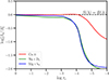 |
Fig. C.1. Departure coefficients for non-LTE spectral lines. This plots shows the dependence with optical depth log τc of the ratio of upper and lower level departure coefficients βu/βl. Color lines correspond to each of the analyzed spectral lines formed under non-LTE conditions: Mg I b2 (blue), Na I D1 (green) and Ca II (red). They were determined for the VALC model and used to initialize the inversion (see Sect. 3.1). The horizontal dashed line indicates the region where βu = βl and therefore the source function S(λ) corresponds to Planck’s function B(λ) (Sect. B). |
We note that the recalculation of the departure coefficients after the first inversion cycle mentioned in Section 3.1, should be done for all observed NLTE lines. However, in practice, this was done only for the Ca II spectral line. The departure coefficients for Mg I and Na I are kept as those arising from the VALC atmosphere in the entire domain. The reason for this is that the recalculation of new departure for these two lines did not led to better fits of the Stokes parameters, and made the convergence of subsequent inversions harder. Although we do not know with certainty the reason for this, we have identified two possible causes for such behaviour.
First, the presence of three-dimensional radiative transfer effects. Both Mg I b2 and Na I D1 are transitions with very high spontaneous emission rate, which means their level populations are dominated by the radiation which can, in principle, come from nearby pixels (e.g. Leenaarts et al. 2010). The coupling of neighboring pixels is a consequence of 3D non-LTE radiative transfer, and our calculation of departure coefficients that treats each pixel as a one-dimensional plane-parallel atmosphere cannot account for this coupling. We stress that, while the Ca II line is also a non-LTE sensitive to such effects (e.g. de la Cruz Rodríguez et al. 2012), it is generally more coupled to local conditions than the Na I and Mg I lines (recall Fig. C.1).
A second possible reason for such a discrepancy is that the atomic models used for the Na I and Mg I lines have been tailored to reproduce the spectral line shapes of the quiet Sun for the VALC atmosphere. Therefore, it is not guaranteed that the re-calculation of the departure coefficients for substantially different atmospheres found in umbra and penumbra will produce the departure coefficients consistent between these two lines, as well as the Ca II line. This effect can be particularly pronounced in the Mg I b2 line as the neutral magnesium, as a minority species, requires the so-called opacity fudge (see e.g., Vukadinović et al. 2022, and references therein). The opacity fudge tables are typically calculated for a particular mean atmosphere model, like VALC, and could prove to be inadequate for other atmosphere models. We stress that our work is one of the few studies that attempt to perform a comprehensive multi-line inversion in a sunspot. Sunspots exhibit significantly different physical conditions (temperature, density, etc.) compared to the quiet Sun, so inadequacies of the atomic model or fudge factors are expected to matter more.
All Tables
All Figures
|
Fig. 1. Representative Stokes profiles at three different locations in the diffraction limited observations. The three locations are: penumbra (green), umbra (blue), umbral flash (red). The points display the observed data whereas solid lines correspond to the fitted profiles. The profiles are normalized to the quiet sun continuum and to better visualize the data, vertical shifts have been applied. These are: [ + 0.2, 0, −0.2] in Stokes I and [ + 0.02, 0, −0.02] in Stokes Q, U and V. In addition, Stokes I signals in the umbra (blue) and umbral flash (red) have been multiplied by a factor of 2 before the shift is applied to better display the variations. |
| In the text | |
|
Fig. 2. Observations and inversion results. Top panels: Maps of the observed intensity at three different wavelengths (from left to right): continuum of the Fe I line at 630 nm, core of the Mg I line at 517 nm, and core of the Ca II line at 854 nm. Middle panels: Temperature inferred from the inversion at three different optical depth levels (from left to right): τc = 1 (photospheric continuum), τc = 10−2.5 (high photosphere), and τc = 10−5 (chromosphere). Bottom panels: Same as middle panels but showing the inferred line-of-sight velocity. Inner and outer blue circles are located at radii r/Rs = 0.4, 1.0, 1.4, respectively, where Rs is defined as the sunspot’s radius as measured from the umbral center (red cross). The direction of the solar disk center is indicated by the bold arrow. Dashed black lines depict a cone of ±15° around the line of symmetry of the spot. |
| In the text | |
|
Fig. 3. Inversion results. Similar to middle and bottom panels of Fig. 2 but displaying the Bx (top), By (middle) and Bz (bottom) components of the magnetic field in the local reference frame at three different optical depths. |
| In the text | |
|
Fig. 4. Average sunspot properties. Azimuthal averages of the physical parameters, as inferred from the Stokes inversion, as a function of the normalized sunspot radius r/Rs at different optical-depth levels: log τc = 0 (red), −1 (orange), −2 (yellow), −3 (green), −4 (blue), −5 (cyan), −6 (purple). Typical deviations around the mean are represented by the vertical colour bars. All panels, except (h) and (i) were produced by averaging over 2π radians. Panels h (vlos in the center side penumbra) and i (vlos in the limb side penumbra) were obtained by averaging only over ±π/12 radians around the sunspot’s line of symmetry (see cone denoted by dashed lines in Figs. 2 and 3). |
| In the text | |
|
Fig. 5. View of the umbral flash inferred from the diffraction limited data. Upper panel: Divided map of temperature T(x, y) (bottom left) and line-of-sight velocity vlos (top right) at z ∼ 1 Mm. The horizontal dotted line represents the slice selected for the three lower panels, and the cross indicates where the umbral flash happens (i.e. where the strongest supersonic velocities are found). Bottom panels: Temperature T(x, z), Mach number M(x, z), and magnetic field B(x, z) on the plane of the slice indicated on the upper panel (y = 88 Mm). As a reference, the curves of constant optical depth log τc = 0, −2, −3, −4, −5 are indicated by the dashed black or white lines. Green contours indicate the regions where supersonic flows are found: ∥M > 1∥. |
| In the text | |
|
Fig. 6. Atmosphere stratification of one of the pixels of the umbral flash with supersonic velocities. From top to bottom: Temperature T, line-of-sight velocity normalized to the local sound speed (i.e. line-of-sight Mach number) vlos/cs, logarithm of density log ρ, and logarithm of gas pressure log Pg. Bottom axis and red lines represent the physical parameters as a function of the optical depth scale log τc, whereas the upper axis and blue lines represent the physical parameters as a function of geometrical height z. We note the continuum (log τc = 0) is formed at around z ≈ 0.2 Mm above the lowermost boundary of the domain. Error estimations inferred from the Stokes inversion are presented for the temperature and velocity as shadowed areas. The horizontal dashed line represents the limit at which the line-of-sight velocity becomes supersonic. |
| In the text | |
|
Fig. A.1. Response functions for the temperature (ℛℱT; upper-left), line-of-sight velocity (ℛℱvlos; upper-right), vertical component of the magnetic field (ℛℱBz; lower-left), and horizontal component of the magnetic field (ℛℱBh; lower-right) for a pixel located in the penumbra as a function of wavelength and optical depth log τc. See text for details. |
| In the text | |
|
Fig. C.1. Departure coefficients for non-LTE spectral lines. This plots shows the dependence with optical depth log τc of the ratio of upper and lower level departure coefficients βu/βl. Color lines correspond to each of the analyzed spectral lines formed under non-LTE conditions: Mg I b2 (blue), Na I D1 (green) and Ca II (red). They were determined for the VALC model and used to initialize the inversion (see Sect. 3.1). The horizontal dashed line indicates the region where βu = βl and therefore the source function S(λ) corresponds to Planck’s function B(λ) (Sect. B). |
| In the text | |
Current usage metrics show cumulative count of Article Views (full-text article views including HTML views, PDF and ePub downloads, according to the available data) and Abstracts Views on Vision4Press platform.
Data correspond to usage on the plateform after 2015. The current usage metrics is available 48-96 hours after online publication and is updated daily on week days.
Initial download of the metrics may take a while.