| Issue |
A&A
Volume 647, March 2021
|
|
|---|---|---|
| Article Number | A98 | |
| Number of page(s) | 11 | |
| Section | Extragalactic astronomy | |
| DOI | https://doi.org/10.1051/0004-6361/202039914 | |
| Published online | 16 March 2021 | |
Spectroscopy and polarimetry of the gravitationally lensed quasar Q0957+561
1
Astronomical Observatory, Volgina 7, 11000 Belgrade, Serbia
e-mail: This email address is being protected from spambots. You need JavaScript enabled to view it.
2
Department of Astronomy, Faculty of Mathematics, University of Belgrade, Studentski trg 16, Belgrade 11000, Serbia
e-mail: This email address is being protected from spambots. You need JavaScript enabled to view it.
3
Special Astrophysical Observatory of the Russian AS, Nizhnij Arkhyz, Karachaevo-Cherkesia 369167, Russia
e-mail: This email address is being protected from spambots. You need JavaScript enabled to view it.
Received:
15
November
2020
Accepted:
18
January
2021
Abstract
Context. We present new spectroscopic and polarimetric observations of the first discovered gravitational lens, Q0957+561. The lensed quasar has been observed with the 6 m telescope of the Special Astrophysical Observatory (Russia) in polarimetric and spectroscopic modes.
Aims. We explore the spectropolarimetric parameters of the A and B components of Q0957+561 to investigate the innermost structure of gravitationally lensed quasars and explore the nature of polarization in lensed quasars. Additionally, we aim to compare their present-day spectral characteristics with previous observations in order to study long-term spectral changes.
Methods. We perform new spectral and polarization observations of the Q0957+561 A and B images. After observed data reduction, we analyse the spectral characteristics of the lensed quasar, comparing the spectra of the A and B images, as well as comparing previously observed image spectra with present-day ones. The polarization parameters of the two images are also compared. Furthermore, we model the macro-lens influence on the polarization of the images, representing the gravitational lens with a singular isothermal elliptical potential.
Results. We find that the brightness and the spectral energy distribution ratio of components A and B have changed over a long period. Polarization in the broad lines of components A and B show that equatorial scattering cannot be detected in this lensed quasar. We find wavelength-dependent polarization that may be explained as a combination of the polarization from the disc and the outflowing material. There is a significant difference between the polarization parameters of the A and B images: The B component shows a higher polarization rate and polarization angle. However, both polarization vectors are nearly perpendicular to the observed radio jet projection. This indicates that the polarization in the continuum comes from the accretion disc. Our simple lensing model of a polarized source shows that, in principle, macro lenses can cause the observed differences in the polarization parameters of the Q0957+561A and B images. Using the Mg II broad line and luminosity of component A, we estimate the Q0957+561 black hole mass to be MSMBH ≈ (4.8 − 6.1) × 108 M⊙.
Key words: gravitational lensing: strong / polarization / quasars: emission lines / quasars: individual: Q957+561 / quasars: supermassive black holes
V. L. Afanasiev passed away on December 21, 2020.
© ESO 2021
1. Introduction
Gravitationally lensed quasars are very important for a number of investigations in astrophysics. First of all, the light from these objects is amplified, and we can detect objects at large redshift; therefore, the investigation of lensed quasars and their geometry (in combination with the foreground galaxy) is important for cosmology. Additionally, gravitational lenses can be used to constrain the innermost structure of lensed quasars (see e.g., Jiménez-Vicente et al. 2014; Braibant et al. 2017; Hutsemékers et al. 2017; Popović et al. 2020), which are a specific class of the active galactic nuclei (AGNs). Different emitting regions (which are of different dimensions) of a lensed quasar can be affected differently by microlensing (see e.g., Jovanović et al. 2008). This can cause chromatic effects (Popović & Chartas 2005) in an image of the lensed quasar spectrum. Therefore, variations in the spectral characteristics of an image of lensed quasars can constrain the quasar’s inner structure (see e.g., Popović et al. 2001; Abajas et al. 2002, 2007; Popović & Chartas 2005; Sluse et al. 2007; Blackburne et al. 2011; Fian et al. 2016, 2018, etc.). For example, the gravitational microlensing effect provides a way to explore the accretion disc structure and its temperature profile (see e.g., Cornachione & Morgan 2020), as well as the structure and kinematics of the broad line region (BLR; see e.g., Popović et al. 2001; Abajas et al. 2002; Sluse et al. 2012; Guerras et al. 2013; Braibant et al. 2017; Hutsemékers et al. 2017), which emits broad lines.
These broad lines originate relatively close to the central supermassive black hole (SMBH), which is assumed to be in the centre of AGNs, and can be used to measure its mass (see Peterson 2014; Mediavilla et al. 2018, 2019; Popović 2020). There is a possibility that the BLR emission is amplified by the microlensing effect, and, consequently, the broad lines can be affected by this effect (see e.g., Popović et al. 2001, 2020; Abajas et al. 2002; Braibant et al. 2017; Hutsemékers et al. 2017; Fian et al. 2018, etc.). This may provide information about the BLR dimension and kinematics.
The BLR structure and kinematics can be investigated by using polarization characteristics across a broad line profile (see e.g., Smith et al. 2004; Afanasiev et al. 2014, 2019; Savić et al. 2018, etc.). As it was shown recently by Afanasiev et al. (2019), polarization in broad lines can be used to explore the BLR kinematics, inclination, and dimensions. Another important finding is that the polarization in broad lines can be used for SMBH mass estimates (see Afanasiev & Popović 2015; Savić et al. 2018; Afanasiev et al. 2019).
Consequently, spectropolarimetric observations can give very useful information about the structure of lensed quasars (see e.g., Hutsemékers et al. 1998, 2015; Belle & Lewis 2000; Hales & Lewis 2007; Popović et al. 2020, etc.). However, the nature of polarization in lensed quasars is not yet clearly understood. Comparing different images of the SDSS J1004+4112 lensed quasar, Popović et al. (2020) found that a significant change in polarization parameters (observed only in component D) can be explained by the microlensing of a scattering region located in the inner part of a dusty torus. Different mechanisms could contribute to the polarization in quasars (Smith et al. 2004), and different effects in the lensed polarized light can be expected. In order to continue our investigation of the spectropolarimetric characteristics of lensed quasars, we observed the lensed quasar Q0957+561 with the 6 m telescope of Special Astrophysical Observatory of the Russian Academy of Science (SAO RAS) in the polarization and spectral modes.
The first identified gravitationally lensed quasar, Q0957+561 (Walsh et al. 1979), has two images of a quasar with redshift z = 1.41 that is lensed by a foreground bright galaxy at z = 0.36 in a cluster of galaxies (see e.g., Gondhalekar & Wilson 1980; Young et al. 1980, 1981; Rhee 1991; Keeton et al. 2000). There are two images, A and B, of a lensed quasar projected at the distance of more than 6″. The spectra of both images show broad emission lines (see e.g., Walsh et al. 1979; Young et al. 1981), which are usually observed in the spectrum of a Type1 quasar. Images A and B have been observed in X-ray (see e.g., Chartas et al. 1995) and radio (see e.g., Greenfield et al. 1985; Garrett et al. 1994; Campbell et al. 1995; Reid et al. 1995; Haarsma et al. 1997, 2008) spectral bands. The time delay between components A and B is around 420−425 days (see e.g., Schild 1990; Beskin & Oknyanskij 1995; Pijpers 1997; Kundić et al. 1997; Oscoz et al. 2001; Ovaldsen et al. 2003; Shalyapin et al. 2008, 2012, etc.). The images of the Q0957+561 quasar have been monitored in different spectral bands (see e.g., Chartas et al. 1995; Campbell et al. 1995; Goicoechea et al. 2008), and investigations of the innermost structure have been performed (see e.g., Schild 2005; Hainline et al. 2012) using the variability of the images. Additionally, polarization in both images has been reported by Dolan et al. (1995).
In Popović et al. (2020), we explored the polarization of a radio-quiet lensed quasar, SDSS J1004+4112, and found significant differences between polarization parameters in different images. However, due to the somewhat lower brightness of the lens components, we could not explore the polarization across the broad line profiles. To explore the polarization in the broad lines of a gravitational lens, one has to select a lens with enough bright and separated images. This motivated us to observe the lensed radio-loud quasar Q0957+561 in the spectroscopic and polarization modes with the 6 m telescope of the SAO observatory.
We obtained spectroscopic and polarimetric observations of Q0957+561 in February and April 2020. The idea was to explore the spectral and polarization characteristics of the lensed quasar and determine the possible influence of macrolensing on the polarization of lensed quasars.
Throughout this paper, we adopt the following cosmological parameters: Ωm = 0.27, ΩΛ = 0.73, and H0 = 71 km s−1 Mpc−1. The paper is organized as follows: In Sect. 2, we describe our observations, and in Sect. 3 we give the results, which are discussed in Sect. 4. The main conclusions are summarized in Sect. 5.
2. Observations and data reduction
The first gravitational quasar lens, Q0957+561, was observed in early 2020 with the 6 m telescope using the universal spectrograph SCORPIO-2 in various modes (Afanasiev & Moiseev 2011). Initially, the task was to study the polarization in broad lines using spectropolarimetric data and measure the mass of the central black hole (see Afanasiev & Popović 2015). However, the obtained polarization angle (PA) shape across the broad Mg II line profile indicated that the equatorial scattering mechanism (typical for Type 1 AGNs; see Smith et al. 2004; Afanasiev et al. 2019) is not dominant. Therefore, we performed additional spectral observations, in non-polarized light with a high signal-to-noise ratio and high-precision photometry and polarimetry, of the Q0957+561 A and B images.
2.1. Spectropolarimetry
For spectropolarimetric observations with SCORPIO-2, we used a double Wollaston prism as an analyser in a parallel beam of a focal reducer. In such an analyser, the beam, divided into two halves, enters two Wollaston prisms, separating the directions of the polarization plane by 0° −90° and 45° −135°, respectively. This allows us to simultaneously register four spectra of an object in four polarization planes and determine the Stokes parameters based on these data. On February 16, 2020, the observations of Q0957+561 were made in this mode under good atmospheric conditions (seeing 1.2″ and variations of the polarization channel transmission of < 1%). The slit width was 2″, and its length was 60″. The slit passed through both images of the lensed quasar (position angle 168°). A series of quasar spectra were obtained with a total exposure of 3900 s and a spectral resolution of 14 Å in the range of 4200−7400 Å (VPHG940@600 grating). Images were registered on the EEV42-90 charge-coupled device (CCD) with the format 4096 × 2048 px (Murzin et al. 2016). On the same night, spectra of the spectropolarimetric standards (G191B2B and BD+59d389 stars) were obtained at close zenith distances to calibrate the transmission of the polarization channels. The techniques of polarization observations, calibration, and data reduction are described in Afanasiev & Amirkhanyan (2012). As a result of the reduction, the spectra of components A and B of the gravitational lens were obtained in four directions of polarization, I0(λ), I90(λ), I45(λ), and I135(λ). In this case, the first three Stokes parameters can be found from the relations:
 (1)
(1)
 (2)
(2)
 (3)
(3)
Here, KQ(λ) and KU(λ) are instrumental parameters that define the dependence of the transmission of spectral channels on the wavelength specified by observations of standard zero-polarization stars.
2.2. Spectrophotometry
Spectra with a high signal-to-noise ratio were obtained on April19, 2020, by the SCORPIO-2 spectrograph in a long-slit mode in the range 3700−7300 Å using VPHG1200@540 grating with good atmospheric transparency and 1.2″ seeing. The six spectra were obtained with a total exposure of 1800 s. The spectral resolution determined from the lines of the night sky was 7.5 Å. We obtained the spectrum of the spectrophotometric standard BD+75d325 at a close zenith distance for absolute flux calibration. The new sensor CCD261−84 2048 × 4096 px with a size of 15 microns was used. This CCD is manufactured with new ‘high-rho’ technology that is used to increase the thickness of the silicon to maximize the response at the infrared end of the spectral range. Such a device, with the exception of its high quantum efficiency (> 90% at 400−900 nm and > 40% at 350 and 1000 nm) in the entire visible range, has practically no fringes (their amplitude is < 0.2%) in the red region (see Jorden et al. 2010). A special feature of the device is the large number of cosmic ray hits registered even at short exposures, which complicates data reduction.
Data reduction was carried out using the standard method for reducing long-slit spectra: construction of a two-dimensional geometric distortion model followed by the bi-linear interpolation of two-dimensional spectra into a rectangular coordinate grid, the linearization and correction of the spectral flat-field, the subtraction of the sky background, the removal of cosmic ray hints, and the extraction of spectra (Afanasiev & Amirkhanyan 2012).
2.3. Photometry and polarimetry
Image polarimetry of the Q0957+561 A and B components was performed on April 24, 2020, with the SCORPIO-2 spectrograph in the g-SDSS and r-SDSS filters. The Wollaston prism was used as an analyser in combination with a rotating half-wave phase plate. The plate rotates at four fixed angles: 0°, 22.5°, 45°, and 67.5°. For each angle, we registered two 3′ × 2′ images on CCD261−84 in two polarization directions, 0° (o-ray) and 90° (e-ray), as shown in Fig. 1. Thirty-two images (eight series of exposures for the four positions of the phase plate) were obtained with an exposure of 200 s. For ordinary Fo and extraordinary Fe rays, the fluxes of the studied objects were measured using aperture photometry on each frame. Then the dimensionless values F = (Fo − Fe)/(Fo + Fe) were calculated. The dimensionless Stokes parameters Q and U can be found from the known relation:
 (4)
(4)
 (5)
(5)
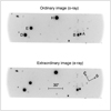 |
Fig. 1. Comparison of ordinary (o-ray) and extraordinary (e-ray) images. |
where θ is the rotation angle of the phase plate.
The variations in the atmospheric transparency during the observations did not exceed 0.5%, and seeing was 1.4−1.7″. Images of the zero-polarization standard BD+32d3739 were also obtained to determine instrumental polarization, and the highly polarized standard Hiltner 960 was observed to control the direction of the PA. The secondary standards in the Q0957+561 field (stars D, E, and H, as shown in Fig. 1) taken from Ovaldsen et al. (2003) were used for the photometric binding. The magnitudes of these stars in the g-SDSS and r-SDSS filters are taken from Shalyapin et al. (2008). In individual frames, the signal-to-noise ratio is 300−400 for the quasar and > 2000 for the reference stars. However, transparency variations can worsen the photometric accuracy, and, for further processing, we used the method of differential photometry and polarimetry, which is described in detail in Shablovinskaya & Afanasiev (2019). To determine the flux, we added the measurements obtained from the two directions of polarization. Thus, 32 independent measurements were made for each object in each filter. Table 1 shows the results of photometry of the Q0957+561 A and B components and the two reference stars D and E relative to the H star.
Photometry of Q0957+561.
3. Results
3.1. Spectral characteristics of the Q0957+561 A and B images
As can be seen from Table 1, the brightness ratio of the B/A components is 1.85 in the blue region of the spectrum and 1.75 in the red. This can be seen clearly in Figs. 2 and 3.
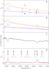 |
Fig. 2. Integral spectra of components A and B of the lensed quasar Q0957+561. Panel a: observed A and B spectra. Panel b: A and B spectra without the absorption lines. Panel c: B/A flux ratio as a function of wavelength. Panel d: emission line spectra of the A and B components after subtracting the continuum. The lines are identified according to Boyle (1990). |
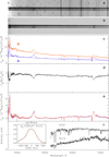 |
Fig. 3. Long-slit spectra of the A and B components of Q0957+561. Panel a: linearized source spectrum. Panel b: sky subtracted spectrum with removed cosmic rays. Panel c: extracted spectra of components A (blue) and B (red) of the lensed quasar image. Panel d: brightness ratio of the components. Panel e: spectra of components A (blue) and B (red) after continuum subtraction. Panel f: spectrum of the lensing galaxy in arbitrary units and the comparison star, shifted by z = 0.36. Panel f (left): also shows the cross-correlation function between the spectra of the star and the lens galaxy. |
Figure 2a shows the integral spectra I(λ) calculated according to Eq. (1) for components A and B and corrected for spectral sensitivity. The spectrum of each component contains the strong broad emission lines CIII] 1909 Å and Mg II 2790 Å as well as the weak blended lines of Fe II multiplets. In the Mg II region, there are narrow metal lines belonging to the quasar and an atmospheric absorption band, O2, which complicates the analysis of the polarization in broad lines and requires that these lines be first removed from the spectrum. Figure 2b shows the spectra with absorption lines removed.
Our spectra (Fig. 2c) clearly show that component B (south) is more than 1.5 times brighter than component A (north), although the brightness ratio of B/A was less than 1 when the Q0957+561 lens system was discovered by Walsh et al. (1979). This ratio changes with the wavelength. Walsh et al. (1979) showed the increase in the B/A ratio with the wavelength, but our observations show that the ratio decreases with the wavelength. As can be seen in Fig. 2c, the brightness ratio of components B and A is 15−20% lower in the emission lines than in the continuum. To understand this, we subtracted a continuum approximated by a power-law dependency λ−α. Estimations of α for components B and A are 1.43 ± 0.10 and 1.07 ± 0.09, respectively. The emission spectrum of both components after subtracting the continuum is presented in Fig. 2d. As can be seen, the component spectra match up to errors, which means that, in the emission lines, the gravitational brightness amplification is not observed in the lens components of Q0957+561. To verify this observing fact, we performed additional spectral observations with a high signal-to-noise ratio, and the results of these observations are shown in Fig. 3.
Figure 3a shows the image of the original linearized spectrum, and Fig. 3b shows the spectrum after subtracting the background and removing cosmic rays. The correction for atmospheric extinction for the spectrophotometric standard and the object was performed in a standard way, taking into account measurements of the spectral transparency of the atmosphere at the 6m telescope location (Kartasheva & Chunakova 1978).
The spectra of the Q0957+561 components corrected for spectral sensitivity are presented in Fig. 3c. Atmospheric absorption in the O2 band is accounted for by the observations of a bright star in the field. The difference in the slope of the component spectra, detected in our first observation (spectropolarimetric mode), can be seen quite confidently. The indexes α for components B and A are equal to 1.41 ± 0.07 and 1.16 ± 0.15, respectively, which corresponds to the spectropolarimetric measurements within the error limits. The ratio Fλ(B)/Fλ(A) shown in Fig. 3d also corresponds to that obtained by spectropolarimetry. The difference of about 5% is due to different image qualities during observations. Figure 3e shows the spectra of both components after subtracting the power-law continuum. The spectra do not reveal any significant difference in the fluxes of emission lines, which confirms the result obtained by spectropolarimetry. In the spectrum of component B, a small increase in intensity is seen in the region of 6000−7000 Å, which is due to a lensing galaxy entering the slit located in 0.6″ in the projection. Figure 3f shows the spectrum of the lensing galaxy as a result of subtracting the spectra of the components, taking into account the difference in their brightness. The same figure shows the spectrum of the HD245 star of the G2V spectral class, taken from the MILES spectrum library (Sánchez-Blázquez et al. 2006). The star spectrum is shifted to z = 0.36. The cross-correlation analysis of the star and the lensing galaxy spectra shown in the rest frame and corrected for spectral resolution is plotted in the left-hand side of Fig. 3f. The Gaussian approximation of the cross-correlation function gives an estimate of the dispersion of stellar velocities in the lens of σ* = 335 ± 31 km s−1. This is in an agreement with the measurements reported by Mediavilla et al. (2000). They obtained a central stellar dispersion of σ* = 310 ± 20 km s−1 for the lens galaxy G1, which is associated with Q0957+561 A and B.
We explored the B/A ratio from previous observations and found that, when the lens was discovered, the initial brightness ratio B/A was 0.76 in the blue part and 1 in the red (Walsh et al. 1979). In the 1980s, Gondhalekar & Wilson (1980) observed the B/A ratio to be around 0.7 in the whole spectral range, and, according to Vanderriest et al. (1989), the B/A ratio in 1980−1983 was between 0.85 and 0.95 in the red part, while it stayed constant in the blue part at the level of 0.5. Measurements of the B/A ratio in papers from the 1990s to 2008 show that the B component stays brighter (i.e. B/A > 1), with the B/A values ranging between 1.05 and 1.22 (see Schild 1990; Colley et al. 2002, 2003; Shalyapin et al. 2008). It is obvious that the B/A ratio is changing, and, consequently, one can expect that the power-law index α also changes over time. To explore the changes of index α for components A and B, we used a spectral database1 of bright lensed quasars (Gil-Merino et al. 2018). We used observations from the Liverpool Robotic Telescope (LRT) obtained in 2015 and our observations with 6 m alt/az mounted telescope (BTA – Big Telescope Alt-azimuth) from 2020. Furthermore, to investigate the behaviour of α, we added the photometric data from Shalyapin et al. (2012), corrected for a ∼417 day delay between the lens components. The relation between the slope α and the flux of each component is plotted in Fig. 4.
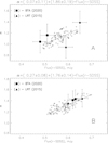 |
Fig. 4. Changes in the slope α as a function of the observed flux for components A (upper panel) and B (lower panel). Open circles denote the photometric data taken from Shalyapin et al. (2012). Solid squares denote our observations (BTA) and solid triangles the observations with LRT given in the database of bright quasars (see Gil-Merino et al. 2018). The BTA and LRT observations were conducted in the spectral mode, which explains the significant errorbars. |
As can be seen in Fig. 4, the slope α is well correlated with the flux for both components. It indicates that the blue part of the spectra is amplified in the brighter phase.
3.2. Polarization of the Q0957+561 A and B images
We found the Stokes parameters Q(λ) and U(λ) and then calculated the polarization degree P(λ) and the angle of the polarization plane φ(λ) as functions of wavelength using the known relations:
![Mathematical equation: $$ \begin{aligned} \begin{aligned}&P(\lambda )=\sqrt{Q(\lambda )^2+U(\lambda )^2},\\&\varphi (\lambda )={1\over 2}\arctan {[{U(\lambda )}/{Q(\lambda )]}}+\varphi _0, \end{aligned} \end{aligned} $$](/articles/aa/full_html/2021/03/aa39914-20/aa39914-20-eq6.gif) (6)
(6)
where φ0 is the zero point determined by observations of a highly polarized standard star. The π/2 ambiguity of the PA is corrected according to the formulae given in Bagnulo et al. (2009).
As it can be seen in Fig. 5, the polarization parameters seem to be different for different components. We could not find the expected ‘S’ shaped profile in broad lines, including the Mg II broad line.
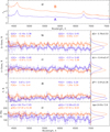 |
Fig. 5. Spectra of the A and B components (panel a) and their polarization parameters as a function of wavelength (panels b–e). Observed Stokes parameters (panels b and c), the degree of polarization (panel d), and the angle of the polarization plane (panel e) for components A (blue) and B (red) of the Q0957+561 lens are shown. The spectropolarimetric data in panels b–e are binned over 40 Å. The left sides of panels b–e show robust estimates for each parameter in the g-SDSS (left) and r-SDSS (right) bands. The right sides of panels b–e show the distribution of parameter values and their average difference for B minus A. |
The first panel in Fig. 5 shows the integral spectra of the A and B components, given for comparison with the polarized spectra presented in panels b–e. In each of panels b–e, the average robust estimates of the polarization parameters and their errors for the g-SDSS (left) and r-SDSS bands (right) are given. The given errors are the robust standard deviations. From top to bottom, we plot the Stokes parameters Q (panel b) and U (panel c) as well as the polarization parameters: the polarization degree in percent (panel d) and the PA (panel e). The data for component B are denoted in red and for component A in blue. All quantities are given as functions of wavelengths.
On the right sides of panels b–e (Fig. 5), the averaged values and distribution of polarization parameters are given. The true accuracy of the estimates of the Stokes parameters and the degree of polarization is about 0.5 ÷ 0.7%, and the accuracy of the angle estimation is 15° ÷25°. The accuracy is affected not only by the value of the measured flux in the polarization channels, but also by variations in the atmospheric depolarization at different exposures and errors of integration of the component spectra. As can be seen in Fig. 5, the accuracy of measuring the polarization parameters is slightly higher for the brighter component B than for A. However, as shown on the right-hand side of the panels in Fig. 5, a statistical difference between the polarization parameter distributions of the A and B components is present.
Table 2 shows the results of measuring the Q0957+561 polarization parameters using image-polarimetry data. There are estimates based on broadband spectropolarimetry data obtained via integration in the g-SDSS and r-SDSS bands. The accuracy of the image polarimetry is ∼0.1−0.2% for the polarization degree and 2−3° for the PA.
Polarimetry of Q0957+561.
The polarimetry data confirm the ∼1.5 times difference in the degree of polarization of components A and B detected by spectropolarimetry. The degree of polarization for each component does not depend on the wavelength within the errorbars. The PA of component B is the same within the errorbars in the blue and red parts of the spectrum and is equal to ∼150°. For componentA, the PA changes along the spectrum: from 130° in the blue region to ∼120° in the red.
The spectra of both components (see e.g., Fig. 2) show the broad lines, for example Mg II, which may come from the partly virialized BLR and, in principle, can be used for mass determination (for a review, see Popović 2020, and reference therein). In Savić et al. (2020), we show that, in the case of the Mg II line where outflows and inflows in far wings can be present, the ‘S’ shaped PA profile across the broad line can still be present. Yet, the ‘S’ shaped PA across Mg II is not present in components A or B. This may indicate that the polarization mechanism is likely not related to the equatorial scattering on the dusty torus (see Savić et al. 2018, 2020).
The polarization of the continuum has an electric vector direction between 120° (component A) and 150° (component B), which is approximately perpendicular to the radio jet axis (see Fig. 6). In Fig. 6, we over-plot the polarization vector (shown as arrows) on the composite radio image of the Q0957+561 lens system taken from Reid et al. (1995). The polarization vector is almost perpendicular to the radio jet observed in component A. Since the λ18 cm global very long baseline interferometry (VLBI) hybrid maps (see Fig. 2 in Garrett et al. 1994) show nearly parallel radio jets of the A and B components on the milliarcsecond scale, it seems that the polarization vector is nearly perpendicular to the radio jet in the source.
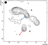 |
Fig. 6. Orientation of the polarization vectors in the A and B components of the Q0957+561 gravitational lens. The vectors (as arrows) are over-plotted on the composite radio image of the lens taken from Reid et al. (1995). |
3.3. SMBH mass of Q0957+561
We were not able to measure the Q0957+561 SMBH mass using the polarization in the broad lines caused by equatorial scattering. However, a combination of spectral and photometric observations allowed us to estimate the absolute values of the emitted flux and, consequently, the mass of the central SMBH.
To do this, we measured the flux of component A, which is farther away from the lensing galaxy and is probably not microlensed, at a wavelength 3000 Å in the reference frame of the lensed quasar: Fλ = (3.2 ± 0.6) × 10−16 erg cm−2 s−1 Å−1. The amplified quasar luminosity is obtained as μ × (λL3000) = (1.2 ± 0.3) × 1046 erg cm−2, where μ is the amplification of component A due to macrolensing.
The amplification estimation was done similarly as in Popović et al. (2020); taking κ ≈ 0.47 (Nakajima et al. 2009) and γ ≈ 0.1 (Fadely et al. 2010; Krips et al. 2005) for component A, we obtained μ = 3.7. The size of the BLR in the Mg II line was estimated using the empirical BLR radius–luminosity (R–L) relation (see Czerny et al. 2019; Popović 2020). We used the updated R–L relation (at 3000 Å) given by Zajaček et al. (2020) and obtained  light days.
After subtracting the Fe II contribution to the Mg II line using the UV Fe II model given in Popović et al. (2019)2, we measured the full width at half maximum FWHM = 3.68 × 10³ km s−1 and estimated the cloud velocity as σ = FWHM/2.355 = 1.58 × 10³ km s−1.
We then used the relation (see Peterson 2014)
 (7)
(7)
where f is a dimensionless parameter equal to 5.5 (Onken et al. 2004), depending on the BLR structure and kinematics and the inclination of the system relative to the observer, G is the gravitational constant, and R is the BLR dimension. We estimated the SMBH mass to be MSMBH ≈ 6.1 × 10⁸ M⊙.
We also estimated the SMBH mass directly using λL3000 and the FWHM of the broad Mg II emission line, according to the relation given in Popović (2020):
 (8)
(8)
where λL3000 is given in units of 1044 erg s−1 and the FWHM is in units of 103 km s−1. Using this relationship, we found the SMBH mass to be MSMBH = 4.8 × 10⁸ M⊙, which is close to the result obtained above. Our SMBH estimates, MSMBH ≈ (4.8 − 6.1) × 108 M⊙, are in agreement with Assef et al. (2011), who obtained (4.7 − 9.5) × 108 M⊙.
We should note that we have assumed that the A component is not microlensed. However, we cannot exclude this possibility, and the obtained SMBH mass may be affected by this phenomenon.
4. Discussion
4.1. Spectral characteristics: Changes in the innermost structure – Intrinsic variability versus microlensing
The B/A flux ratio shows that component B is brighter than A in our observations as well as in observations made after the 1990s. However, in the epoch of lensed quasar discovery (Walsh et al. 1979) and the following several years, component A was brighter in the UV spectra than component B (Gondhalekar & Wilson 1980; Vanderriest et al. 1989). We also found that there is a relationship between the change in the B/A ratio and slope α. When the images stay brighter, the blue part of their spectra stays more intense (see Fig. 4). Additionally, Shalyapin et al. (2012) found that the flux ratio oscillated in the g-SDSS and r-SDSS bands during their observations, and that the ratio showed a slight increase during periods of violent variability.
This variability, which causes the changes in the spectral energy distribution (SED) in the UV band, is probably due to perturbations of the inner quasar structure. It is known that the temperature of the accretion disc can change due to variations in the accretion rate (see Koratkar & Blaes 1999), and this will have an influence on the UV SED changes.
However, one cannot exclude the influence of microlensing on the observed changes in the UV SED. As is well known, the microlensing effect is in principle achromatic, but if the dimensions of a disc (or a disc corona) are wavelength-dependent (i.e. the temperature varies across the disc; see Jovanović et al. 2008), then one can expect the microlensing effect to be chromatic (see Popović & Chartas 2005), which would be observed as different amplifications in different wavelength bands (see Jovanović et al. 2008).
One can expect an intrinsic variability that is dominant in component A since the optical depth for the microlensing of component A should be significantly smaller than that of component B (component B is projected very close to the lens galaxy). One can also assume that any extra variability detected in component B is due to microlensing. The amplification of the component B continuum seen today (which is brighter than that of component A by about a factor of two) is probably caused (at least partly) by microlensing since there is no line intensity variability (see Fig. 2d), which is expected in the case of intrinsic variability. The line shapes and their flux ratio are the same. Since the BLR is significantly larger than the continuum source, the caustic can amplify the continuum source but not the BLR emission (see Abajas et al. 2002).
The conclusion from the spectral observations is that the change in the component A spectra is mostly caused by the intrinsic variability of the quasar. However, the variability in the component B spectra is more complex: Both intrinsic variability and the microlensing of the continuum source can contribute to the observed variability. The amplification of component B is also reported in Gil-Merino et al. (2018), where B/A > 1 was observed after 2011−2012 (see their Fig. 6). Moreover, Belete et al. (2019) found that component B has been microlensed in recent epochs (after 2011, similar to Gil-Merino et al. 2018).
4.2. Polarization of Q0957+561 components A and B
4.2.1. Polarization mechanisms in the lensed source
We expected to observe polarization in the Q0957+561 A and B broad line profiles, which is typical for Type 1 AGNs that show dominant equatorial scattering (see e.g., Smith et al. 2004; Afanasiev & Popović 2015; Afanasiev et al. 2019). However, as can be seen in Fig. 5 (panel e), the ‘S’ shaped profiles of the PA in broad CIV and Mg II lines are not present (as is expected in Type 1 AGNs; see Savić et al. 2018, 2020).
The absence of an ‘S’ shaped PA profile may indicate that: (a) There is no equatorial scattering of the BLR light, and (b) the Keplerian motion is not dominant in the BLR. However, different BLR geometries produce different shapes in the PA and different polarization degrees in the broad lines. This is also the case of the BLR with an outflow component (see Savić et al. 2020) that is expected to be in the BLR emitting Mg II and CIV lines (see Popović et al. 2020; Popović 2020). However, as can be seen in Fig. 3, the polarization and PA in the broad lines are on the level of the continuum (within the errorbars).
This indicates that some other effect may be present, such as depolarization due to a hot region located above the BLR. A similar effect is found in 3C390.3 (see Afanasiev et al. 2015), which is a radio-loud AGN. This may also be the case for Q0957+561 since the lensed quasar is a radio-loud object and there are two radio components corresponding to the A and B images (see Greenfield et al. 1985; Roberts et al. 1985). Therefore, we can expect some outflow of hot gas above the BLR as well as significant depolarization. Furthermore, Schild (2005) indicated, the bi-conical structures located above and below the plane of the accretion disc, which is apparently inclined at 55° to the line of sight.
An alternative explanation for the broad line polarization absence is that the equatorial scattering is still present in the inner part of the torus. However, if the BLR dimension is comparable with the inner radius of the torus, the polarization in the broad lines cannot be detected (see Kishimoto et al. 2004).
The polarization in the continuum seems to be wavelength-dependent, showing a larger degree of polarization at shorter wavelengths. The degree of polarization and the PA are different in the A and B components. Previously, Dolan et al. (1995) found that the polarization in both components should be P ≤ 3.2% (taking a 2σ upper limit), which is comparable with our measurements that show the polarization on the level of 1%.
The observed continuum polarization in Q0957+561 may be due to electron scattering originating in the atmosphere of a plane-parallel scattering-dominated disc. In this case, the vector of the electric field is perpendicular to the symmetry axis of the disc, and the disc axis is assumed to be along the jet direction (Kishimoto et al. 2003) However, the polarization in the continuum can partly come from the central accretion disc and partly from the synchrotron radiation of the optical continuum in the jet.
If the polarized continuum is coming from the accretion disc, one can expect the electric vector to be perpendicular to the jet. Figure 6 shows that the vector of the electric field seems to be perpendicular to the projected jet direction of component A, indicating that the polarization probably originates in the accretion disc (see e.g., Kishimoto et al. 2003). However, the problem is explaining the wavelength-dependent polarization if there is only polarization connected with the accretion disc. There are several ideas regarding the observed wavelength-dependent polarization in some AGNs (see Webb et al. 1993; Beloborodov 1998). One possibility is that polarization in the accretion disc, or in the ‘hot corona’ (assumed to be around the disc) in combination with outflow can give wavelength-dependent polarization (see Beloborodov 1998). The Lyα of Q0957+561 A and B shows a P Cyg profile (see e.g., Dolan et al. 1995; Popović & Chartas 2005) that indicates an outflow in hot gas, supporting this scenario.
4.2.2. Polarization and the gravitational lensing effect
As we discussed in Sect. 3.2, it is obvious that there are differences between the polarization parameters of the A and B images. There is a difference in the PA of the A and B components of around ΔφAB ∼ 20°. The difference between the radio jet projections of component A compared to that of component B is smaller, Δθ ∼ 10°, but still exists (see Fig. 5 in Gorenstein et al. 1988). This difference in the A and B jet angle projections can also be seen in Barkana et al. (1999, see their Fig. 1) and in Haarsma et al. (2008, see their Fig. 2). This may indicate two possible scenarios. The first is that the difference in the PA is caused by the macro-lens (and/or microlensing) effect of the continuum source. Otherwise, a difference in the PA between the components may be caused by the jet-disc precession since the time delay between components A and B is around 420 days (see Shalyapin et al. 2008, 2012). This time delay may be long enough to see two positions of the jet-disc system.
We cannot expect the gravitational lens to produce an additional polarization effect of a polarized source (see Kronberg et al. 1991). However, the gravitational distortion can change the observed polarization parameters, especially in the source where the polarization depends on the dimensions of the emitting region (as for example in the case of microlensing; see Popović et al. 2020). In the radio-loud quasars, the continuum polarization can have two contributing components, one coming from a disc and a synchrotron polarization component coming from the jet. Considering the dimension of these two regions, microlensing can affect the polarization component coming from the disc (the disc dimension is comparable with the Einstein radius ring – ERR – for microlensing; see Popović et al. 2020), and macrolensing may affect the polarization parameters coming from more extensive sources, such as the jet emission (the jet dimension can be comparable to ERR for macrolensing; see Kronberg et al. 1991). The quasar jet emission is most intense in the radio, but a smaller fraction of the jet emission (usually highly polarized) can contribute to the optical part. Therefore, one can expect both gravitational macro- and microlensing to produce an additional effect on the observed polarization of lensed images.
In Popović et al. (2020), we demonstrate the microlensing effects of polarized light due to the equatorial scattering. This can qualitatively be applied to other polarization mechanisms where the polarization parameters depend on the dimensions of a polarization region or the anisotropy of the polarization source. Additionally, here we explore the influence of macrolensing on the observed polarization in different images.
To demonstrate the influence of the strong lensing on the polarization signal, particularly on the PA, we modelled the emitting region as an ellipsoidal source (jet-like structure; see the left-hand sides of the panels in Fig. 7). We assumed that the polarization vector has an orientation of α = 90° to the ellipsoid orientation. The polarization of the source follows the surface intensity (taken to have a distribution: the red colour in Fig. 7 indicates higher intensity, the blue lower intensity), and the total polarization degree is P = 0.58%. The lens is represented by singular isothermal elliptic (SIE) potential (for analytic forms for the SIE potential, see Kassiola & Kovner 1993; Kormann et al. 1994; Keeton & Kochanek 1998).
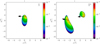 |
Fig. 7. Model of an extended jet-like polarized source (left) that is affected by the gravitational lens (right). The parameters for the macro lens are taken as for the Q0951+561 lens system. Small black lines show the distribution and orientation of the electric vector (lengths correspond to the rate of polarization as shown on the plots). The large arrows show only the orientation of the polarization vector, and the colours indicate the intensity in arbitrary units (blue showing smaller intensities). |
In Fig. 7 (right panel), we obtained two images of extended structure, with total polarization around P = 1.42% in both images, but the PA between the two images has a difference of Δα ∼ 14°. Therefore, the difference between the PAs in the images is probably caused by the macro lens, but the polarization degree is expected to be similar in both images.
We note here that the averaged PAs of the components (shown as large arrows) do not significantly change the orientation with respect to the PA of the source, and therefore the observed PA in both images is probably perpendicular to the observed radio jet. Here we used a simple model for an extensive source in order to see the distribution of the electric vector and find a total PA, but a similar effect can be expected if the polarization is combined from two sources: one from a disc (which is dominant) and another highly polarized light from a jet with a small contribution. As a final effect, the polarization of the disc will be affected by the polarized light from the extensive jet, which is amplified differently by macrolensing. This may be an explanation of the observed difference in the polarization parameters of the Q0957+561 A and B images.
Additionally, we cannot exclude that the microlensing is causing the difference between polarization parameters in images A and B. The microlensing affects the polarization of compact regions with anisotropic polarization. This effect is qualitatively similar to the case of equatorial scattering shown in Popović et al. (2020). However, it is hard to disentangle macrolensing and microlensing effects from one epoch observation (or two very close epochs). Therefore, future polarization observations are needed to clarify this issue.
As we noted above, the second scenario may be that the observed difference in the PA is caused by the disc-jet precession. However, the VLBI observations obtained at different epochs show the same orientation of the jet in images A and B (see Haarsma et al. 1997, 2008); therefore, it is unlikely that the jet precession is present.
5. Conclusions
We have presented spectroscopic and polarimetric observations of the lensed quasar Q0957+561 obtained with the 6 m SAO RAS telescope. We analysed our observations from two epochs, and we compared our observations with previous ones. From our analysis, we can conclude the following:
-
The B/A ratio during both epochs was around two, which indicates a strong magnification of component B. Both images show a bluer spectrum as brightness becomes stronger; this effect is probably mostly caused by the intrinsic variability in the quasar. However, there is a difference in this change in component B compared to component A. The interval in the change of component B seems to be larger than in component A. This indicates that, in addition to the intrinsic variation, microlensing probably contributes to the brightness of component B.
-
Polarization in the broad lines is not present, and it is (within the errorbars) on the level of the continuum. Therefore, the equatorial scattering is probably not dominant in the broad lines. This may indicate two possible effects: The first is the complete lack of equatorial scattering, and the second is the presence of a depolarization region above the BLR. Moreover, an absorption observed in the Lyα line indicates an outflowing BLR, which may be a depolarization region located between the observer and the BLR. An alternative scenario for the lack of polarization in the broad lines is that the inner equatorial scattering region is comparable with an outer BLR radius.
-
The polarization in both components seems to be wavelength-dependent, and the polarization vector is almost perpendicular to the observed radio jet. This indicates that the continuum polarization may come from the accretion disc, and that there are some effects that are causing the wavelength-dependent polarization (see e.g., Webb et al. 1993; Beloborodov 1998).
-
The polarization parameters between the A and B components of Q0957+561 are different. Using a sample model of a polarized extensive source, we show that gravitational macrolensing could explain these differences. However, we cannot exclude some other effects, such as microlensing.
-
Using the Mg II FWHM and λL(3000 Å) from the high quality spectrum of component A, we found the Q0957+561 SMBH mass to be MSMBH ≈ (4.8 − 6.1) × 108 M⊙.
The polarization effect in the lensed quasar Q957+561 seems to have a different nature than in SDSS J1004+411. It seems that in the case of Q957+561, the macrolensing effect contributes to the detected difference in the PA between components A and B.
Models of the UV Fe II can be found at http://servo.aob.rs/FeII_AGN/link7.html
Acknowledgments
This work is supported by the Ministry of Education, Science and Technological Development of R. Serbia (the contract 451-03-68/2020-14/200002). VLA and ESS thank the grant of Russian Science Foundation project number 20-12-00030 “Investigation of geometry and kinematics of ionized gas in AGNs by polarimetry methods”, which supported the spectropolarimetric and polarimetric observations and data analyze. Observations with the SAO RAS telescopes are supported by the Ministry of Science and Higher Education of the Russian Federation (including agreement No 05.619.21.0016, project ID RFMEFI61919X0016). We would like to thank the referee for giving very useful comments which helped improving the quality of the paper.
References
- Abajas, C., Mediavilla, E., Muñoz, J. A., Popović, L. Č., & Oscoz, A. 2002, ApJ, 576, 640 [NASA ADS] [CrossRef] [Google Scholar]
- Abajas, C., Mediavilla, E., Muñoz, J. A., Gómez-Alvarez, P., & Gil-Merino, R. 2007, ApJ, 658, 748 [NASA ADS] [CrossRef] [Google Scholar]
- Afanasiev, V. L., & Amirkhanyan, V. R. 2012, Astrophys. Bull., 67, 438 [NASA ADS] [CrossRef] [Google Scholar]
- Afanasiev, V. L., & Moiseev, A. V. 2011, Balt. Astron., 20, 363 [NASA ADS] [Google Scholar]
- Afanasiev, V. L., & Popović, L. Č. 2015, ApJ, 800, L35 [Google Scholar]
- Afanasiev, V. L., Popović, L. Č., Shapovalova, A. I., Borisov, N. V., & Ilić, D. 2014, MNRAS, 440, 519 [Google Scholar]
- Afanasiev, V. L., Shapovalova, A. I., Popović, L. Č., & Borisov, N. V. 2015, MNRAS, 448, 2879 [NASA ADS] [CrossRef] [Google Scholar]
- Afanasiev, V. L., Popović, L. Č., & Shapovalova, A. I. 2019, MNRAS, 482, 4985 [NASA ADS] [CrossRef] [Google Scholar]
- Assef, R. J., Denney, K. D., Kochanek, C. S., et al. 2011, ApJ, 742, 93 [NASA ADS] [CrossRef] [Google Scholar]
- Bagnulo, S., Landolfi, M., Landstreet, J. D., et al. 2009, PASP, 121, 993 [NASA ADS] [CrossRef] [Google Scholar]
- Barkana, R., Lehár, J., Falco, E. E., et al. 1999, ApJ, 520, 479 [NASA ADS] [CrossRef] [Google Scholar]
- Belete, A. B., Canto Martins, B. L., Leão, I. C., & De Medeiros, J. R. 2019, MNRAS, 484, 3552 [Google Scholar]
- Belle, K. E., & Lewis, G. F. 2000, PASP, 112, 320 [NASA ADS] [CrossRef] [Google Scholar]
- Beskin, G. M., & Oknyanskij, V. L. 1995, A&A, 304, 341 [NASA ADS] [Google Scholar]
- Beloborodov, A. M. 1998, ApJ, 496, L105 [NASA ADS] [CrossRef] [Google Scholar]
- Blackburne, J. A., Pooley, D., Rappaport, S., & Schechter, P. L. 2011, ApJ, 729, 34 [NASA ADS] [CrossRef] [Google Scholar]
- Boyle, B. J. 1990, MNRAS, 243, 231 [NASA ADS] [Google Scholar]
- Braibant, L., Hutsemékers, D., Sluse, D., & Goosmann, R. 2017, A&A, 607, A32 [NASA ADS] [CrossRef] [EDP Sciences] [Google Scholar]
- Campbell, R. M., Lehar, J., Corey, B. E., Shapiro, I. I., & Falco, E. E. 1995, AJ, 110, 2566 [NASA ADS] [CrossRef] [Google Scholar]
- Czerny, B., Olejak, A., Rałowski, M., et al. 2019, ApJ, 880, 46 [Google Scholar]
- Chartas, G., Falco, E., Forman, W., et al. 1995, ApJ, 445, 140 [Google Scholar]
- Colley, W. N., Schild, R. E., Abajas, C., et al. 2002, ApJ, 565, 105 [Google Scholar]
- Colley, W. N., Schild, R. E., Abajas, C., et al. 2003, ApJ, 587, 71 [NASA ADS] [CrossRef] [Google Scholar]
- Cornachione, M. A., & Morgan, C. W. 2020, ApJ, 895, 93 [Google Scholar]
- Dolan, J. F., Michalitsianos, A. G., Thompson, R. W., et al. 1995, ApJ, 442, 87 [NASA ADS] [CrossRef] [Google Scholar]
- Fadely, R., Keeton, C. R., Nakajima, R., & Bernstein, G. M. 2010, ApJ, 711, 246 [NASA ADS] [CrossRef] [Google Scholar]
- Fian, C., Mediavilla, E., Hanslmeier, A., et al. 2016, ApJ, 830, 149 [NASA ADS] [CrossRef] [Google Scholar]
- Fian, C., Guerras, E., Mediavilla, E., et al. 2018, ApJ, 859, 50 [NASA ADS] [CrossRef] [Google Scholar]
- Garrett, M. A., Calder, R. J., Porcas, R. W., Walsh, D., & Wilkinson, P. N. 1994, MNRAS, 270, 457 [NASA ADS] [CrossRef] [Google Scholar]
- Gil-Merino, R., Goicoechea, L. J., Shalyapin, V. N., & Oscoz, A. 2018, A&A, 616, A118 [NASA ADS] [CrossRef] [EDP Sciences] [Google Scholar]
- Goicoechea, L. J., Shalyapin, V. N., Gil-Merino, R., & Ullán, A. 2008, A&A, 492, 411 [EDP Sciences] [Google Scholar]
- Gondhalekar, P., & Wilson, R. 1980, Nature, 285, 461 [Google Scholar]
- Gorenstein, M. V., Cohen, N. L., Shapiro, I. I., et al. 1988, ApJ, 334, 42 [NASA ADS] [CrossRef] [Google Scholar]
- Greenfield, P. D., Roberts, D. H., & Burke, B. F. 1985, ApJ, 293, 370 [Google Scholar]
- Guerras, E., Mediavilla, E., Jimenez-Vicente, J., et al. 2013, ApJ, 764, 160 [NASA ADS] [CrossRef] [Google Scholar]
- Haarsma, D. B., Hewitt, J. N., Lehár, J., & Burke, B. F. 1997, ApJ, 479, 102 [NASA ADS] [CrossRef] [Google Scholar]
- Haarsma, D. B., Winn, J. N., Shapiro, I., & Lehár, J. 2008, AJ, 135, 984 [Google Scholar]
- Hainline, L. J., Morgan, C. W., Beach, J. N., et al. 2012, ApJ, 744, 104 [NASA ADS] [CrossRef] [Google Scholar]
- Hales, C. A., & Lewis, G. F. 2007, PASA, 24, 30 [NASA ADS] [CrossRef] [Google Scholar]
- Hutsemékers, D., Lamy, H., & Remy, M. 1998, A&A, 340, 371 [Google Scholar]
- Hutsemékers, D., Sluse, D., Braibant, L., & Anguita, T. 2015, A&A, 584, A61 [NASA ADS] [CrossRef] [EDP Sciences] [Google Scholar]
- Hutsemékers, D., Braibant, L., Sluse, D., Anguita, T., & Goosmann, R. 2017, Front. Astrophys. Space Sci., 4, 18 [Google Scholar]
- Jiménez-Vicente, J., Mediavilla, E., Kochanek, C. S., et al. 2014, ApJ, 783, 47 [NASA ADS] [CrossRef] [Google Scholar]
- Jorden, P. R., Downing, M., Harris, A., et al. 2010, Proc. SPIE, 7742, 77420J [Google Scholar]
- Jovanović, P., Zakharov, A. F., Popović, L. Č., & Petrović, T. 2008, MNRAS, 386, 397 [NASA ADS] [CrossRef] [Google Scholar]
- Kartasheva, T. A., & Chunakova, N. M. 1978, Astrofizicheskie Issledovaniia Izvestiya Spetsial’noj Astrofizicheskoj Observatorii, 10, 44 [NASA ADS] [Google Scholar]
- Kassiola, A., & Kovner, I. 1993, ApJ, 417, 450 [NASA ADS] [CrossRef] [Google Scholar]
- Keeton, C. R., & Kochanek, C. S. 1998, ApJ, 495, 157 [NASA ADS] [CrossRef] [Google Scholar]
- Keeton, C. R., Falco, E. E., Impey, C. D., et al. 2000, ApJ, 542, 74 [NASA ADS] [CrossRef] [Google Scholar]
- Kishimoto, M., Antonucci, R., & Blaes, O. 2003, MNRAS, 345, 253 [NASA ADS] [CrossRef] [Google Scholar]
- Kishimoto, M., Antonucci, R., Boisson, C., & Blaes, O. 2004, MNRAS, 354, 1065 [NASA ADS] [CrossRef] [Google Scholar]
- Koratkar, A., & Blaes, O. 1999, PASP, 111, 1 [NASA ADS] [CrossRef] [Google Scholar]
- Kormann, R., Schneider, P., Bartelmann, M., et al. 1994, A&A, 284, 285 [Google Scholar]
- Krips, M., Neri, R., Eckart, A., et al. 2005, A&A, 431, 879 [NASA ADS] [CrossRef] [EDP Sciences] [Google Scholar]
- Kronberg, P. P., Dyer, C. C., Burbidge, E. M., & Junkkarinen, V. T. 1991, ApJ, 367, L1 [Google Scholar]
- Kundić, T., Turner, E. L., Colley, W. N., et al. 1997, ApJ, 482, 75 [NASA ADS] [CrossRef] [Google Scholar]
- Mediavilla, E., Serra-Ricart, M., Oscoz, A., Goicoechea, L., & Buitrago, J. 2000, ApJ, 531, 635 [NASA ADS] [CrossRef] [Google Scholar]
- Mediavilla, E., Jiménez-Vicente, J., Fian, C., et al. 2018, ApJ, 862, 104 [NASA ADS] [CrossRef] [Google Scholar]
- Mediavilla, E., Jiménez-Vicente, J., Mejía-Restrepo, J., et al. 2019, ApJ, 880, 96 [CrossRef] [Google Scholar]
- Murzin, V. A., Markelov, S. V., Ardilanov, V. I., et al. 2016, Adv. Appl. Phys., 4, 50 [Google Scholar]
- Nakajima, R., Bernstein, G. M., Fadely, R., Keeton, C. R., & Schrabback, T. 2009, ApJ, 697, 1793 [NASA ADS] [CrossRef] [Google Scholar]
- Onken, C. A., Ferrarese, L., Merritt, D., et al. 2004, ApJ, 615, 645 [NASA ADS] [CrossRef] [Google Scholar]
- Oscoz, A., Alcalde, D., Serra-Ricart, M., et al. 2001, ApJ, 552, 81 [NASA ADS] [CrossRef] [Google Scholar]
- Ovaldsen, J. E., Teuber, J., Schild, R. E., & Stabell, R. 2003, A&A, 402, 891 [NASA ADS] [CrossRef] [EDP Sciences] [Google Scholar]
- Peterson, B. M. 2014, Space Sci. Rev., 183, 253 [NASA ADS] [CrossRef] [Google Scholar]
- Pijpers, F. P. 1997, MNRAS, 289, 933 [NASA ADS] [CrossRef] [Google Scholar]
- Popović, L. Č. 2020, Open Astron., 29, 1 [Google Scholar]
- Popović, L. Č., & Chartas, G. 2005, MNRAS, 357, 135 [NASA ADS] [CrossRef] [Google Scholar]
- Popović, L. Č., Mediavilla, E. G., & Muõz, J. A. 2001, A&A, 378, 295 [NASA ADS] [CrossRef] [EDP Sciences] [Google Scholar]
- Popović, L. Č., Kovačević-Dojčinović, J., & Marčeta-Mandić, S. 2019, MNRAS, 484, 3180 [NASA ADS] [CrossRef] [Google Scholar]
- Popović, L. Č., Afanasiev, V. L., Moiseev, A., et al. 2020, A&A, 634, A27 [EDP Sciences] [Google Scholar]
- Rhee, G. 1991, Nature, 350, 211 [Google Scholar]
- Reid, A., Shone, D. L., Akujor, C. E., et al. 1995, A&AS, 110, 213 [NASA ADS] [Google Scholar]
- Roberts, D. H., Greenfield, P. E., Hewitt, J. N., Burke, B. F., & Dupree, A. K. 1985, ApJ, 293, 356 [Google Scholar]
- Sánchez-Blázquez, P., Peletier, R. F., Jiménez-Vicente, J., et al. 2006, MNRAS, 371, 703 [NASA ADS] [CrossRef] [Google Scholar]
- Savić, D., Goosmann, R., Popović, L. Č., Marin, F., & Afanasiev, V. L. 2018, A&A, 614, A120 [NASA ADS] [CrossRef] [EDP Sciences] [Google Scholar]
- Savić, D., Popović, L. Č., Shablovinskaya, E., & Afanasiev, V. L. 2020, MNRAS, 497, 3047 [Google Scholar]
- Schild, R. E. 1990, AJ, 100, 1771 [NASA ADS] [CrossRef] [EDP Sciences] [Google Scholar]
- Schild, R. E. 2005, AJ, 129, 1225 [NASA ADS] [CrossRef] [Google Scholar]
- Shablovinskaya, E. S., & Afanasiev, V. L. 2019, MNRAS, 482, 4322 [Google Scholar]
- Shalyapin, V. N., Goicoechea, L. J., Koptelova, E., Ullän, A., & Gil-Merino, R. 2008, A&A, 492, 401 [NASA ADS] [CrossRef] [EDP Sciences] [Google Scholar]
- Shalyapin, V. N., Goicoechea, L. J., & Gil-Merino, R. 2012, A&A, 540, A132 [NASA ADS] [CrossRef] [EDP Sciences] [Google Scholar]
- Sluse, D., Claeskens, J.-F., Hutsemekers, D., & Surdej, J. 2007, A&A, 468, 885 [NASA ADS] [CrossRef] [EDP Sciences] [Google Scholar]
- Sluse, D., Hutsemékers, D., Courbin, F., Meylan, G., & Wambsganss, J. 2012, A&A, 544, A62 [NASA ADS] [CrossRef] [EDP Sciences] [Google Scholar]
- Smith, J. E., Robinson, A., Alexander, D. M., et al. 2004, MNRAS, 350, 140 [Google Scholar]
- Vanderriest, C., Schneider, J., Herpe, G., et al. 1989, A&A, 215, 1 [NASA ADS] [Google Scholar]
- Walsh, D., Carswell, R. F., & Weymann, R. J. 1979, Nature, 279, 381 [NASA ADS] [CrossRef] [PubMed] [Google Scholar]
- Webb, W., Malkan, M., Schmidt, G., & Impey, C. 1993, ApJ, 419, 494 [NASA ADS] [CrossRef] [Google Scholar]
- Young, P., Gunn, J. E., Kristian, J., Oke, J. B., & Westphal, J. A. 1980, ApJ, 241, 507 [NASA ADS] [CrossRef] [Google Scholar]
- Young, P., Gunn, J. E., Kristian, J., Oke, J. B., & Westphal, J. A. 1981, ApJ, 244, 736 [NASA ADS] [CrossRef] [Google Scholar]
- Zajaček, M., Czerny, B., Martinez-Aldama, M. L., et al. 2020, ApJ, 896, 146 [CrossRef] [Google Scholar]
All Tables
All Figures
|
Fig. 1. Comparison of ordinary (o-ray) and extraordinary (e-ray) images. |
| In the text | |
|
Fig. 2. Integral spectra of components A and B of the lensed quasar Q0957+561. Panel a: observed A and B spectra. Panel b: A and B spectra without the absorption lines. Panel c: B/A flux ratio as a function of wavelength. Panel d: emission line spectra of the A and B components after subtracting the continuum. The lines are identified according to Boyle (1990). |
| In the text | |
|
Fig. 3. Long-slit spectra of the A and B components of Q0957+561. Panel a: linearized source spectrum. Panel b: sky subtracted spectrum with removed cosmic rays. Panel c: extracted spectra of components A (blue) and B (red) of the lensed quasar image. Panel d: brightness ratio of the components. Panel e: spectra of components A (blue) and B (red) after continuum subtraction. Panel f: spectrum of the lensing galaxy in arbitrary units and the comparison star, shifted by z = 0.36. Panel f (left): also shows the cross-correlation function between the spectra of the star and the lens galaxy. |
| In the text | |
|
Fig. 4. Changes in the slope α as a function of the observed flux for components A (upper panel) and B (lower panel). Open circles denote the photometric data taken from Shalyapin et al. (2012). Solid squares denote our observations (BTA) and solid triangles the observations with LRT given in the database of bright quasars (see Gil-Merino et al. 2018). The BTA and LRT observations were conducted in the spectral mode, which explains the significant errorbars. |
| In the text | |
|
Fig. 5. Spectra of the A and B components (panel a) and their polarization parameters as a function of wavelength (panels b–e). Observed Stokes parameters (panels b and c), the degree of polarization (panel d), and the angle of the polarization plane (panel e) for components A (blue) and B (red) of the Q0957+561 lens are shown. The spectropolarimetric data in panels b–e are binned over 40 Å. The left sides of panels b–e show robust estimates for each parameter in the g-SDSS (left) and r-SDSS (right) bands. The right sides of panels b–e show the distribution of parameter values and their average difference for B minus A. |
| In the text | |
|
Fig. 6. Orientation of the polarization vectors in the A and B components of the Q0957+561 gravitational lens. The vectors (as arrows) are over-plotted on the composite radio image of the lens taken from Reid et al. (1995). |
| In the text | |
|
Fig. 7. Model of an extended jet-like polarized source (left) that is affected by the gravitational lens (right). The parameters for the macro lens are taken as for the Q0951+561 lens system. Small black lines show the distribution and orientation of the electric vector (lengths correspond to the rate of polarization as shown on the plots). The large arrows show only the orientation of the polarization vector, and the colours indicate the intensity in arbitrary units (blue showing smaller intensities). |
| In the text | |
Current usage metrics show cumulative count of Article Views (full-text article views including HTML views, PDF and ePub downloads, according to the available data) and Abstracts Views on Vision4Press platform.
Data correspond to usage on the plateform after 2015. The current usage metrics is available 48-96 hours after online publication and is updated daily on week days.
Initial download of the metrics may take a while.