© ESO 2021

1. Introduction

Binary decisions inevitably have to be made at the conclusion of a physical experiment. These include whether or not a feature has been detected significantly, which model describes the data better, and whether datasets (or subsets thereof) are consistent with each other or are in ‘tension’, which could be a potential indicator for new physics not incorporated in the model.

Traditionally, hypothesis tests were the statistical tools of choice to answer these questions. With the advent of high-performance computing, Bayesian techniques building on Bayesian evidence have risen in popularity (e.g. Jaffe 1996; Kunz et al. 2006; Marshall et al. 2006; see Trotta 2008 for a review). In cosmology, discrepancies in the ∼3−5σ range between high-redshift observations – primarily the cosmic microwave background (CMB), as constrained most accurately by the Planck mission; Planck Collaboration VI 2020 – as well as various probes of the low-redshift universe in the measurement of the Hubble constant (e.g. Riess et al. 2016, 2018, 2019; Wong et al. 2020) and the amplitude of matter density fluctuations (e.g. Joudaki et al. 2017, 2020; Abbott et al. 2018; Asgari et al. 2020; Heymans et al. 2021) have recently emerged (cf. Verde et al. 2019 for an overview). This has spurred a flurry of work on approaches to quantifying tension and performing model comparison (e.g. Verde et al. 2013; Seehars et al. 2014; Lin & Ishak 2017; Charnock et al. 2017; Köhlinger et al. 2019; Handley & Lemos 2019a; Nicola et al. 2019; Adhikari & Huterer 2019; Raveri & Hu 2019).

What these methods have in common is that they infer a single scalar that is then compared against a predefined scale to judge significance. In Bayesian statistics, the tension measure is conditioned on the observed data. The posterior probability of the parameters, p, of a model, M_i, for measured data, d, is

$$\begin{array}{c}\hfill \mathrm{Pr}(\mathit{p}|\mathit{d},M_i)=\frac{1}{{\mathcal{Z}}_i}\mathrm{Pr}(\mathit{d}|\mathit{p},M_i)\mathrm{Pr}(\mathit{p}|M_i),\end{array}$$(1)

where Pr(d|p, M_i) is the likelihood and Pr(p|M_i) the prior on the model parameters. The Bayesian evidence, or marginal likelihood, is the normalisation given by

$$\begin{array}{c}\hfill {\mathcal{Z}}_i\equiv \mathrm{Pr}(\mathit{d}|M_i)={\displaystyle \int }{\mathrm{d}}^{m}p\mathrm{Pr}(\mathit{d}|\mathit{p},M_i)\mathrm{Pr}(\mathit{p}|M_i),\end{array}$$(2)

where m denotes the number of parameters. For a given dataset, 𝒵_i reduces to a non-stochastic scalar that attains larger values the more likely the realisation of the data is under model M_i, and the more predictive the model is (as a more flexible model could accommodate many possible forms of the data).

However, a physical experiment generally does not take acquired data as a given, but rather interprets them as a stochastic realisation of an underlying truth that we wish to approximate by our model. A different realisation of the data leads to a different value for 𝒵_i, which could alter our decision on tension or consistency. In this view, statistical uncertainty in the data turns the evidence (or any related tension and model comparison measure) into a noisy statistic¹. Jenkins & Peacock (2011) argued, based on toy experiments and analytical arguments, that the thus-inherited statistical uncertainty in 𝒵_i is substantial. Ignoring this scatter will therefore lead to over-confident or incorrect decisions in model comparison.

In this work we quantify the scatter in the Bayesian evidence and some of its derived tension or model comparison statistics, affirming the findings of Jenkins & Peacock (2011) in a realistic cosmological experiment. We devise a computationally efficient procedure to calculate statistical errors on the evidence, apply it to an analysis of internal consistency in Kilo Degree Survey (KiDS) weak lensing data, and explore the impact of data compression on evidence scatter using Planck CMB data as an example.

2. Noisy model comparison

Figure 1 illustrates the notion of evidence and its associated scatter using a Gaussian toy model that is one-dimensional in both data and parameter space. It builds on Fig. 28.6 of MacKay (2003). While at the observed data Model 1 has higher evidence in this example, it is not unambiguously superior because alternative realisations of the data under the more probable Model 1 could result in equal or reversed evidence values of Models 1 and 2 instead (see the boxes in blue and red shading)². We seek to quantify this statistical uncertainty of the evidence (see also Appendix A for a closed-form analytic calculation in the Gaussian case analogous to Fig. 1).

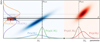Fig. 1. Illustration of model comparison via evidence and of its associated scatter for a one-dimensional data vector d and two models, Mi with i = 1, 2, each with a single parameter p. The joint distributions Pr(d,p|Mi) are shown in blue and red shades. The projections of these distributions onto the parameter and data axes yield the prior Pr(p|Mi) and the evidence or marginal likelihood, respectively (shown in purple and orange for M1 and M2). An experiment produces the observation d, shown as the solid black line. Conditioning on d yields the posterior Pr(p|d,Mi), shown in green and brown for M1 and M2. Evaluating the marginal likelihood at d yields Pr(d|Mi), which is used in the model comparison. The dotted horizontal lines mark the 1σ interval of possible alternative realisations of the data given the best-fit parameter pbest (dashed vertical lines) of either model. The blue and red boxes show the resulting 1σ range in possible evidence values under M1, which has higher evidence in this case (the corresponding ranges for M2 are shown as hatched areas).

2.1. Scatter in the evidence and the Bayes factor

The standard statistic to compare two models, i and j, is the Bayes factor (see Kass & Raftery 1995 for a review),

$$\begin{array}{c}\hfill R_{\mathit{ij}}\equiv \frac{\mathrm{Pr}(M_i|\mathit{d})}{\mathrm{Pr}(M_j|\mathit{d})}=\frac{{\mathcal{Z}}_i\mathrm{Pr}(M_i)}{{\mathcal{Z}}_j\mathrm{Pr}(M_j)}=\frac{{\mathcal{Z}}_i}{{\mathcal{Z}}_j},\end{array}$$(3)

which, for equal prior probabilities of the models themselves, is given by the ratio of the model evidence values. Here, R_ij has the intuitive interpretation of betting odds in favour of model i over j. We shall assume initially that we know the true underlying model, M_true, including its parameters, p_true, that generates the data we observe, which need not coincide with those from either M_i or M_j. Then the probability density of the Bayes factor is given by

$$\begin{array}{c}\hfill \mathrm{Pr}(R_{\mathit{ij}}|M_{\mathrm{true}})={\displaystyle \int }{\mathrm{d}}^{n}d\prime \mathrm{Pr}(R_{\mathit{ij}}|{\mathit{d}}^{\prime })\mathrm{Pr}({\mathit{d}}^{\prime }|M_{\mathrm{true}}),\end{array}$$(4)

where n is the dimension of the data vector, Pr(d|M_true) is the true likelihood of the data, and Pr(R_ij|d) is the distribution of R_ij for a given dataset, which we shall assume to be deterministic. Hence, if the true likelihood is known, we can proceed as follows to create a distribution of R_ij: (i) generate samples of the data from the true likelihood, and (ii) calculate the Bayes factor for each sample according to Eqs. (2) and (3).

As a realistic example, we chose a recent cosmological analysis of tomographic weak lensing measurements by the KiDS survey (KiDS-450; Kuijken et al. 2015; Hildebrandt et al. 2017). We worked with a simulated data vector that, like the real data, has size n = 130 and depends in a highly non-linear way on seven model parameters (five cosmological parameters of a flat ΛCDM model, plus two parameters describing the astrophysical effects on the observables). It was assumed that the data have a Gaussian likelihood with a known and fixed covariance. To perform an internal consistency test, we created two copies of the parameter set and assigned one copy to the elements of the data vector that is dependent on tomographic bin no. 3 and the other copy to the remaining elements. The model comparison is then between the analysis with the original set of model parameters (Model 0) and that with the doubled parameter set (Model 1). Details regarding the methodology and analysis are available in Köhlinger et al. (2019) and Appendix B of this Letter.

We generated 100 realisations of the data vector from the true likelihood, evaluated at a fiducial choice of the parameters. For each simulated data vector, we repeated a full nested sampling analysis of both models (0 and 1) and inferred the evidence (see Appendix B for an assessment of the robustness of the sampling algorithms). By default, we did not introduce any systematic shift into our simulated data; as such, strong concordance is expected as the outcome of the tension analysis.

The resulting distribution of evidence values is shown in Fig. 2. We computed the true value of the Bayes factor by re-running the analyses for a noise-free data vector generated for the fiducial parameter values. The two evidence distributions are each consistent with being lognormal³, each with a standard deviation in the log of 7.9. The evidence is strongly correlated (Pearson correlation coefficient 0.99), which is plausible as the scatter derives from the same noisy data realisation, with both models yielding good fits.

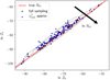Fig. 2. Joint distribution of the evidence calculated under two models (the mock KiDS cosmology analysis for a joint [Model 0] and a split [Model 1] data vector). The arrow indicates the direction of the increasing Bayes factor, lnR01, with the red line marking the true value of R01. Black points correspond to the inferences from 100 noise realisations of the mock data vector, evaluated on the full nested sampling analysis, and the blue points correspond to the ${\chi }_{\text{min}}^2$ approximation from Sect. 3. Contours show the Gaussian kernel density approximation of the distribution based on the black points.

Due to the strong correlation, the distribution of the Bayes factor is narrower, with σ(lnR₀₁) ≈ 1.25 (see Fig. 3 for its distribution). We also observe skewness in lnR₀₁ (already visible in Fig. 2), which causes the mean to be lower relative to the true value by ∼1σ. We do not find evidence that the skewness is due to numerical issues and so ascribe it to the non-linearity of the models; this means that this feature will be strongly dependent on the details of the analysis. A value of σ(lnR₀₁) ∼ 1 is in excellent agreement with the conclusions of Jenkins & Peacock (2011), although they predicted a normal distribution for lnR₀₁ (see also Appendix A).

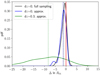Fig. 3. Probability density of the Bayes factor, lnR01, shifted to have its true value at 0. The black curve is the distribution of ΔlnR01 extracted from the full nested sampling analysis, and the blue curve is the distribution extracted from the ${\chi }_{\text{min}}^2$ approximation from Sect. 3. The green curve corresponds to the highly discrepant case of one of four tomographic redshift bins being shifted by dz = 0.3. Dotted lines mark the mean of each distribution.

2.2. Impact on suspiciousness

By design, the Bayes factor depends on the parameter prior, which can be a hindrance for tension assessment, as demonstrated by Handley & Lemos (2019a). They proposed a modified statistic called ‘suspiciousness’, defined as lnS_ij ≡ lnR_ij + D_KL, i − D_KL, j, where

$$\begin{array}{c}\hfill D_{\mathrm{KL},i}={\displaystyle \int }{\mathrm{d}}^{m}p\mathrm{Pr}(\mathit{p}|\mathit{d},M_i)ln\frac{\mathrm{Pr}(\mathit{p}|\mathit{d},M_i)}{\mathrm{Pr}(\mathit{p},M_i)}\end{array}$$(5)

is the Kullback-Leibler (KL) divergence (Kullback & Leibler 1951; see Lemos et al. 2020 for a generalisation to correlated datasets, which we consider here). This combination of evidence and KL divergence is independent of the prior widths, providing they do not impinge upon the posterior bulk, and may be calibrated into a traditional ‘σ tension’ value.

Again assuming a Gaussian likelihood, lnS_ij is χ²-distributed with the degrees of freedom given by the difference in the effective dimension of the parameter space in the two models. Handley & Lemos (2019b) propose calculating this effective dimension as

$$\begin{array}{c}\hfill m_{\mathrm{eff},i}=2\{{\langle {[ln\mathrm{Pr}(\mathit{p}|\mathit{d},M_i)]}^2\rangle }_{\mathrm{p}}-\langle ln\mathrm{Pr}(\mathit{p}|\mathit{d},M_i){\rangle }_{\mathrm{p}}^2\},\end{array}$$(6)

that is, twice the variance of the log-likelihood evaluated over the posterior distribution (indicated by the subscript ‘p’).

We extracted lnS_ij from the output of our nested sampling analysis and determined the scatter of m_eff from the sub-sample variance computed on a posterior sample. The standard deviations of lnR₀₁ and lnS₀₁ agree to better than 10%; the following section outlines an argument for why the distributions of R and S are expected to be very similar. The standard deviation of m_eff is of the order of 10% and can be treated as being uncorrelated with S (correlation coefficient −0.17).

There are two obstacles to using the above approach on real data: (i) repeating full likelihood analyses that include evidence calculations many times to build a sample is prohibitively expensive, and (ii) we do not know the true likelihood to generate samples of the real data. We will address both these points in Sects. 3 and 4.

2.3. Strong tension case

To investigate a case of strong tension, we inserted a large shift, dz = 0.3, into the mean redshift of tomographic bin no. 3 of the simulated data vectors and repeated the analysis⁴. In this case the alternative model 1 is clearly preferred (lnR₀₁ ≈ −23). The impact on the distribution of lnR₀₁ is dramatic, as can be seen from Fig. 3. While the skewness and corresponding discrepancy between the mean and true values persist, the standard deviation increases to 7.3, spanning more than three orders of magnitude in odds.

This result is driven by an increase in the scatter of the evidence (to 10.8 and 8.5 for models 0 and 1, respectively) and in particular by their partial de-correlation (correlation coefficient 0.74). As shown by Jenkins & Peacock (2011), the scatter in lnR_ij is, to a good approximation, proportional to the typical difference between the model predictions at the respective best-fit parameters of the models under comparison (as also shown in Appendix A). This difference is small in our concordant case with nested models, deviating from zero only through scatter in the data. In the dz = 0.3 case, the best fits of the models now lie far apart; this enlarges the scatter and propagates the noise differently into the evidence for models 0 and 1, thereby reducing their correlation.

3. A fast approximate algorithm

We now consider the Laplace approximation of the log-likelihood (we dropped the explicit dependence on the model for simplicity)⁵,

$$\begin{array}{c}\hfill ln\mathrm{Pr}(\mathit{d}|\mathit{p})\approx ln\mathrm{Pr}(\mathit{d}|{\mathit{p}}_0)-\frac{1}{2}{(\mathit{p}-{\mathit{p}}_0)}^{\tau }\mathtt{F}({\mathit{p}}_0)(\mathit{p}-{\mathit{p}}_0),\end{array}$$(7)

where we expanded around the maximum of the log-likelihood at p₀ and introduced the Fisher matrix,

$$\begin{array}{c}\hfill {\mathtt{F}}_{\alpha \beta }=-\langle {\frac{{\partial }^{2}ln\mathrm{Pr}(\mathit{d}|\mathit{p})}{\partial p_{\alpha }\partial p_{\beta }}|}_{{\mathit{p}}_0}\rangle ,\end{array}$$(8)

as the negative expectation of the Hessian of the log-likelihood at p₀. With this approximation the evidence reads

$$\begin{array}{c}\hfill \mathcal{Z}\approx \frac{{(2\pi )}^{m/2}\mathrm{Pr}(\mathit{d}|{\mathit{p}}_0)}{\sqrt{det\mathtt{F}({\mathit{p}}_0)}{V}_{\mathrm{prior}}},\end{array}$$(9)

where we additionally assumed that the prior is uninformative (i.e. the bulk of the likelihood lies well within the volume covered by the prior, denoted as V_prior). Considering a Gaussian likelihood, such that $\text{Pr}(\mathit{d}|{\mathit{p}}_0)\propto {\text{e}}^{-\frac{1}{2}{\chi }^2({\mathit{p}}_0)}$, one finds (cf. Handley & Lemos 2019a)

$$\begin{array}{cc}\hfill ln\mathcal{Z}& \approx \text{const.}-ln{V}_{\mathrm{prior}}-\frac{1}{2}lndet\mathtt{F}({\mathit{p}}_0)-\frac{1}{2}{\chi }^2({\mathit{p}}_0)\text{and}\hfill \end{array}$$(10)

$$\begin{array}{cc}\hfill D_{\mathrm{KL}}& \approx ln{V}_{\mathrm{prior}}-\frac{m}{2}(1+ln2\pi )+\frac{1}{2}lndet\mathtt{F}({\mathit{p}}_0).\hfill \end{array}$$(11)

We see that the only source of scatter is due to the best-fit parameter set p₀, which varies with the noise realisation of the data. If we further assume that the curvature of the likelihood does not vary strongly as the best-fit position moves, only the last term in Eq. (10) is relevant for the statistical uncertainty in ln 𝒵, while D_KL is robust to the scatter. Since ln 𝒵 + D_KL ≈ const. − χ²(p₀)/2, lnS has identical noise properties to ln 𝒵 under these assumptions.

Equipped with these considerations, we propose the following algorithm: (i) perform a single full likelihood analysis and determine fiducial evidence values, 𝒵_fid; (ii) generate samples of the data from the likelihood; (iii) determine the maximum of the likelihood, or equivalently ${\chi }_{\text{min}}^2$, for each sample⁶; and (iv) derive samples of the evidence via

$$\begin{array}{c}\hfill ln{\mathcal{Z}}_{\mathrm{approx},i}:=ln{\mathcal{Z}}_{\mathrm{fid}}-\frac{1}{2}({\chi }_{\min ,i}^2-{\chi }_{\min ,\mathrm{fid}}^2).\end{array}$$(12)

Following this procedure with 100 samples results in the blue points shown in Fig. 2 and the blue distribution in Fig. 3. Apart from sampling noise in the tail, we recover the true distribution well, with the mean and variance in agreement within ∼10%. The change from a full exploration of the posterior, which typically runs in hours to days, to a maximisation of the likelihood, which usually takes minutes to hours, makes exploring the noise properties of the Bayesian evidence and its derived quantities feasible.

4. Evidence samples from real data

When analysing real data, the true likelihood Pr(d′|M_true) found in Eq. (4) needed to generate new copies of the data vector is unavailable. Our best guess for this truth is the best-fitting model, which itself carries uncertainty as it is inferred from the data. In this case we can make use of the posterior predictive distribution (PPD; Gelman et al. 1996), Pr(d′|d, M_k), which yields new samples of the data d′ for a given observation d assuming model M_k (see Trotta 2007 for a very similar application of the PPD). Averaging over all models using the posterior model probabilities Pr(M_k|d) from Eq. (3) then yields

$$\begin{array}{c}\hfill \mathrm{Pr}({\mathit{d}}^{\prime }|M_{\mathrm{true}})\approx \mathrm{Pr}({\mathit{d}}^{\prime }|\mathit{d})={\displaystyle \sum _k\mathrm{Pr}({\mathit{d}}^{\prime }|\mathit{d},M_k)\mathrm{Pr}(M_k|\mathit{d}).}\end{array}$$(13)

The algorithm presented in Sect. 3 therefore only needs to be adjusted in Step (ii), where instead of generating data realisations from the true likelihood in the mock scenario, they are now produced from the PPD via random selection of a subset of posterior samples and evaluation of the likelihood at the parameter values corresponding to these samples.

In practice, we simplified the approach by choosing the model that yields the higher evidence to produce the PPD samples rather than full model averaging. If both models have similar evidence, this choice should have little impact; if the evidence ratio is large, the model with higher evidence is more accurate and/or more predictive (cf. the solid and hatched regions in Fig. 1).

5. Application to KiDS-450 internal consistency

We then inserted the real KiDS-450 data vector into our analysis and generated ten PPD samples from the joint Model 0 as this yields significantly higher evidence than the split model. The derived standard deviations of lnR and lnS are shown in Fig. 4. These statistical errors far exceed the typically quoted ‘method’ errors, which derive from the finite sampling of the posterior. The interpretation of the suspiciousness acquires an additional, albeit smaller, source of error through the effective model dimension, m_eff, that determines the σ-levels.

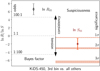Fig. 4. Tension statistics for the case of KiDS-450 internal consistency with respect to tomographic bin no. 3. Shown are the Bayes factor lnR01, with odds ratios, as well as the suspiciousness lnS01, with tension significance, in multiples of the width of an equivalent Gaussian, σ. The smaller red and black error bars are the errors associated with the nested sampling, while the larger orange and grey error bars are the statistical errors derived in this work. Red bands show the statistical uncertainty in determining the σ-levels for lnS01.

The noise in the tension statistics leads to a more conservative evaluation of discrepancies in the data. While the point estimate suggests tension at 1.6σ, this reduces to 1.1σ if we require that all but 16% (i.e. the one-sided tail beyond 1σ of a normal distribution) of possible realisations of the data are discrepant by at least that level. Visually, this corresponds to the upper 1σ error of lnS almost touching the lower limit of the 1σ band in Fig. 4.

6. Benefits of data compression

Planck CMB data are at the centre of both current major tension controversies in cosmology. A practical obstacle to applying our formalism is the complexity of the Planck temperature likelihood, which is assumed to be Gaussian only for ℓ > 30 and builds on pixelised sky maps on larger scales (Planck Collaboration V 2020). This makes drawing PPD samples challenging. However, Prince & Dunkley (2019) recently showed that the low-ℓ likelihood can be efficiently compressed into two Gaussian-distributed band powers. They proceeded to apply maximal, linear compression (using the Multiple Optimised Parameter Estimation and Data or MOPED scheme, Tegmark et al. 1997; Heavens et al. 2000) to the full temperature likelihood and demonstrated it to be nearly lossless. This is not unexpected since the cosmological sampling parameters in CMB analyses are chosen to be close to linear and to be Gaussian-distributed (Kosowsky et al. 2002).

There is an additional motivation to apply data compression: It can suppress scatter in the Bayesian evidence. Under the assumptions outlined in Sect. 3, the statistical properties of ln 𝒵 are driven by the distribution of χ²(p₀) (i.e. the minimum χ²; cf. Eq. (10)). If the data are approximately Gaussian and well fitted by a model whose parameters are close to linear, χ²(p₀) follows a χ²-distribution with N_d.o.f. = n − m degrees of freedom, so that Var(ln 𝒵) = 2N_d.o.f.. Data compression decreases n and can yield N_d.o.f. ≈ 0 in the maximal case, that is, evidence becomes essentially noise-free because a good model with n linear parameters perfectly fits n compressed data. Appendix A demonstrates this explicitly for the Gaussian case.

This may seem paradoxical because compression can at best preserve information, raising the question of how it can facilitate a more precise determination of evidence. In the context of Fig. 1, compression reduces the scatter between the model parameter and the data, so that for a given parameter the data vary little and thus the evidence is known precisely. Conversely, a broad likelihood and/or a high-dimensional data vector lead(s) to large variations in possible realisations of data. While this has no bearing on the posterior, and therefore on the information content, it increases the probability that a certain level of tension or model preference is owed to a particularly (un)lucky noise realisation of the data vector and does not reflect a physical trend.

As a proof of concept, we adopted the Prince & Dunkley (2019) approach, using the provided software⁷, and compressed the Planck temperature anisotropy power spectra into the six cosmological parameters of a spatially flat ΛCDM model (nuisance parameters are marginalised over pre-compression). We then determined the ${\chi }_{\text{min}}^2$ for the compressed real data, as well as for new data realisations generated from the compressed likelihood. We find an extremely small ${\chi }_{\text{min}}^2$ (≈1.4 × 10⁻⁸) for the real data and similar values for the noise realisations, with a standard deviation of 4.4 × 10⁻⁹. Hence, practically noise-free evidence measurements from Planck are indeed possible.

7. Conclusions

We studied the impact on model comparison statistics if these are to be interpreted based on the ensemble of possible observations rather than a single observed realisation of the data. In this setting they become noisy quantities, which affects binary decisions on signal detection, model selection, and tension between experiments. Confirming earlier analytic arguments, we found standard deviations of order unity for the logarithm of the Bayes factor and the suspiciousness statistic, with substantially broader distributions in the case of strong discrepancies between the models under comparison. We expect these conclusions to apply to most, possibly all, informative tension metrics available in the literature as they typically depend on the maximum likelihood or χ²-like expressions.

We proposed a method to approximate the probability distribution of the evidence via repeated draws of mock data from the likelihood, with the maximum likelihood for each mock dataset then obtained, that will add negligible computation time to a full exploration of the posterior distribution. Conclusions drawn from noisy model comparison measures inevitably become more conservative, for example, the tension significance according to the suspiciousness for an internal consistency analysis of KiDS weak lensing data reduces from 1.6σ in the traditional approach to 1.1σ when scatter is accounted for. While in this application the two models under comparison were nested, our formalism and conclusions also hold for the more general case in which parameter spaces differ.

Finally, we demonstrated that data compression suppresses the impact of noisy data on the evidence, in the case of Planck CMB constraints to negligible levels. In light of this, the following pre-processing steps are beneficial before any form of model comparison: (i) compress the data vector as much as possible as long as the compression is essentially lossless; and (ii) choose a parametrisation such that the model is close to linear in the parameters (see e.g. Schuhmann et al. 2016), which increases the chances of achieving a near-perfect fit for any noise realisation of the data.

Acknowledgments

We thank C. Jenkins, J. Peacock, and R. Trotta for insightful discussions. We are also grateful to J. Peacock for a thorough review of the manuscript and to C. Heymans for alerting us to the work of Jenkins and Peacock. BJ acknowledges the kind hospitality of IPMU where part of this work was carried out. FK acknowledges support from the World Premier International Research Center Initiative (WPI), MEXT, Japan. PL acknowledges STFC Consolidated Grant ST/R000476/1. The KiDS analysis is based on observations made with ESO Telescopes at the La Silla Paranal Observatory under programme IDs177.A-3016, 177.A-3017, 177.A-3018, 179.A-2004, 298.A-5015, and on data products produced by the KiDS Consortium.

References

Appendix A: The complete Gaussian case

If we assume that an experiment produces a single observation of n data points⁸ drawn from a Gaussian distribution about some true mean $\overline{\mathit{d}}$ with covariance C,

$$\begin{array}{c}\hfill ln\mathrm{Pr}(\mathit{d})=-\frac{1}{2}ln|2\pi \mathtt{C}|-\frac{1}{2}{(\mathit{d}-\overline{\mathit{d}})}^{\tau }{\mathtt{C}}^{-1}(\mathit{d}-\overline{\mathit{d}}).\end{array}$$(A.1)

In general we do not know $\overline{\mathit{d}}$ but design a model, M, that parameterises the data by some function f(p), with m ≪ n parameters, in the hope that the true data are well approximated by our model. Assuming a given model, the likelihood becomes

$$\begin{array}{c}\hfill ln\mathrm{Pr}(\mathit{d}|\mathit{p},M)=-\frac{1}{2}ln|2\pi \mathtt{C}|-\frac{1}{2}{[\mathit{d}-\mathit{f}(\mathit{p})]}^{\tau }{\mathtt{C}}^{-1}[\mathit{d}-\mathit{f}(\mathit{p})].\end{array}$$(A.2)

A likelihood can often be approximated as a Gaussian in the parameter space,

$$\begin{array}{c}\hfill ln\mathrm{Pr}(\mathit{d}|\mathit{p},M)=ln{L}_{\max }-\frac{1}{2}{(\mathit{p}-\mathit{\mu })}^{\tau }{\mathrm{\Sigma }}^{-1}(\mathit{p}-\mathit{\mu }),\end{array}$$(A.3)

with mean μ and covariance Σ, and the corresponding log-evidence reads

$$\begin{array}{c}\hfill ln\mathcal{Z}\equiv ln\mathrm{Pr}(\mathit{d}|M)=ln{L}_{\max }+ln\frac{\sqrt{|2\pi \mathrm{\Sigma }|}}{V_{\mathrm{prior}}},\end{array}$$(A.4)

where V_prior is the volume of a uniform prior fully encompassing the posterior. One can make the link between Eqs. (A.2) and (A.3) explicit by assuming that we can model our function f as linear in the region of parameter space around p_* where the likelihood is significantly non-zero,

$$\begin{array}{c}\hfill \mathit{f}(\mathit{p})\approx \mathit{f}({\mathit{p}}_{\ast })+\mathrm{\nabla }\mathit{f}({\mathit{p}}_{\ast })(\mathit{p}-{\mathit{p}}_{\ast })=:\widehat{\mathit{d}}+\mathtt{J}(\mathit{p}-{\mathit{p}}_{\ast }),\end{array}$$(A.5)

from which one can identify

$$\begin{array}{cc}\hfill ln{L}_{\max }& =-\frac{1}{2}ln|2\pi \mathtt{C}|-\frac{1}{2}{(\mathit{d}-\widehat{\mathit{d}})}^{\tau }{\stackrel{\sim }{\mathtt{C}}}^{-1}(\mathit{d}-\widehat{\mathit{d}})\text{and}\hfill \end{array}$$(A.6)

$$\begin{array}{cc}\hfill {\mathrm{\Sigma }}^{-1}& ={\mathtt{J}}^{\tau }{\mathtt{C}}^{-1}\mathtt{J};\mathit{\mu }={\mathit{p}}_{\ast }+\mathrm{\Sigma }{\mathtt{J}}^{\tau }{\mathtt{C}}^{-1}(\mathit{d}-\widehat{\mathit{d}}),\hfill \end{array}$$(A.7)

where we defined

$$\begin{array}{c}\hfill {\stackrel{\sim }{\mathtt{C}}}^{-1}:={\mathtt{C}}^{-1}-{\mathtt{C}}^{-1}\mathtt{J}\mathrm{\Sigma }{\mathtt{J}}^{\tau }{\mathtt{C}}^{-1}.\end{array}$$(A.8)

As an aside, Eq. (A.7) shows that noisy data realisations affect the posterior mean but not its covariance. In other words, while the posterior shape is unaffected, the distribution moves as a whole in parameter space with different realisations of the data.

From the above expressions we can immediately see that the evidence is quite a noisy statistic, driven by the second term in Eq. (A.6). Taking the variance of Eq. (A.4) after inserting Eq. (A.6) and assuming that d follows the distribution of Eq. (A.1) yields

$$\begin{array}{c}\hfill \mathrm{Var}(ln\mathcal{Z})=\frac{1}{2}\text{Tr}\left[{({\stackrel{\sim }{\mathtt{C}}}^{-1}\mathtt{C})}^2\right]+{(\overline{\mathit{d}}-\widehat{\mathit{d}})}^{\tau }{\stackrel{\sim }{\mathtt{C}}}^{-1}\mathtt{C}{\stackrel{\sim }{\mathtt{C}}}^{-1}(\overline{\mathit{d}}-\widehat{\mathit{d}}).\end{array}$$(A.9)

The first term here is equal to $\frac{1}{2}(n-m)$, and hence the variance in the raw evidence is large for n ≫ m, even in the event of a good fit to the data (i.e. $\widehat{\mathit{d}}\approx \overline{\mathit{d}}$). We also see that in the case of heavily compressed data, n ∼ m, the evidence scatter reduces considerably.

To derive the expression (A.9), as well as some of the following equations, it is helpful to note that for a Gaussian-distributed variable x with covariance C centred on zero (Petersen & Pedersen 2012),

$$\begin{array}{cc}\hfill ⟨{(\mathit{x}-\mathit{a})}^{\tau }\mathtt{A}(\mathit{x}-\mathit{a})⟩& =\text{Tr}\left[\mathtt{A}\mathtt{C}\right]+{\mathit{a}}^{\tau }\mathtt{A}\mathrm{and}\hfill \\ \hfill \mathrm{Cov}[{(\mathit{x}-\mathit{a})}^{\tau }\mathtt{A}(\mathit{x}-\mathit{a}),{(\mathit{x}-\mathit{b})}^{\tau }\mathtt{B}(\mathit{x}-\mathit{b})]& =2\text{Tr}\left[\mathtt{A}\mathtt{C}\mathtt{B}\mathtt{C}\right]+4{\mathit{b}}^{\tau }\mathtt{B}\mathtt{C}\mathtt{A}\mathit{a},\hfill \end{array}$$(A.10)

where A and B are symmetric matrices, and a and b are arbitrary, non-stochastic vectors.

We are of course really interested in how model comparison (i.e. a difference in evidence) scatters with noisy data, so we introduced two models, one with with ${\widehat{\mathit{d}}}_1$ and J₁ and one with ${\widehat{\mathit{d}}}_2$ and J₂⁹, and asked what the variance in their evidence difference is. Under the true distribution of Eq. (A.1), we find that the log Bayes factor (under the same assumptions as in Eq. (3)), lnR₁₂ = ln 𝒵₁ − ln 𝒵₂, has a mean

$$\begin{array}{cc}\hfill ⟨ln{R}_{12}⟩=& \frac{1}{2}{(\overline{\mathit{d}}-{\widehat{\mathit{d}}}_2)}^{\tau }{\stackrel{\sim }{\mathtt{C}}}_2^{-1}(\overline{\mathit{d}}-{\widehat{\mathit{d}}}_2)-\frac{1}{2}{(\overline{\mathit{d}}-{\widehat{\mathit{d}}}_1)}^{\tau }{\stackrel{\sim }{\mathtt{C}}}_1^{-1}(\overline{\mathit{d}}-{\widehat{\mathit{d}}}_1)\hfill \\ \hfill & +\frac{1}{2}\text{Tr}\left[\mathrm{\Delta }\right]+ln\frac{\sqrt{|2\pi {\mathrm{\Sigma }}_1|}{V}_{\mathrm{prior},2}}{\sqrt{|2\pi {\mathrm{\Sigma }}_2|}{V}_{\mathrm{prior},1}},\hfill \end{array}$$(A.11)

(see also Lazarides et al. 2004; Heavens et al. 2007 for similar, less general expressions) and a variance

$$\begin{array}{c}\hfill \mathrm{Var}(ln{R}_{12})=\frac{1}{2}\text{Tr}\left[{\mathrm{\Delta }}^2\right]+{(\mathrm{\Delta }\overline{\mathit{d}}-\delta )}^{\tau }{\mathtt{C}}^{-1}(\mathrm{\Delta }\overline{\mathit{d}}-\delta ),\end{array}$$(A.12)

where we defined

$$\begin{array}{c}\hfill \mathrm{\Delta }:=\mathtt{C}({\stackrel{\sim }{\mathtt{C}}}_2^{-1}-{\stackrel{\sim }{\mathtt{C}}}_1^{-1});\delta :=\mathtt{C}({\stackrel{\sim }{\mathtt{C}}}_2^{-1}{\widehat{\mathit{d}}}_2-{\stackrel{\sim }{\mathtt{C}}}_1^{-1}{\widehat{\mathit{d}}}_1).\end{array}$$(A.13)

The mean in Eq. (A.11) has three portions: a set of misfit terms on the first line, a constant trace term equal to $\frac{1}{2}(m_1-m_2)$, and an Occam factor. The trace contribution can be understood as a typically small modification of the Occam factor.

In the variance (Eq. (A.12)), there is a trace term that is roughly the dimensionality of the parameter space(s) $\le \frac{1}{2}(m_1+m_2)$, as well as a data misfit term. The trace term is always present, representing the ‘order unity’ term for the general Gaussian case, but can reduce towards zero (via a cross-term that is dependent on both models), getting closer to zero the more similar the two model parametrisations (as quantified by J) are to each other. As opposed to the variance of the evidence (cf. Eq. (A.9)), the trace term in the variance of the Bayes factor does not depend on n, so if n ≫ m, the scatter in R₁₂ is significantly smaller than the scatter in either 𝒵₁ or 𝒵₂ if the data is well fitted. This is the situation we encountered in Fig. 2.

The second term can be small if the models are good, but can also become arbitrarily large, which corresponds to the scatter seen in Fig. 3. It should be noted that in the event of large misfits, the mean and variance are both of the same order, which gives a Poisson-type evidence error associated with measurement noise. This is reassuring as it means the evidence in theory becomes relatively less noisy the larger it becomes. We note that if Eq. (A.5) is a reasonable approximation, provided one can compute (by numerical derivatives or otherwise) the Jacobian J, one may use Eq. (A.12) to evaluate the expected scatter, for example by employing the observed data vector as an estimate of the true $\overline{\mathit{d}}$.

Finally, we offer some illustration for the use of information regarding the sampling distribution of the Bayes factor (such as the variance of Eq. (A.12)) by invoking the popular analogy with betting odds. Rather than placing one’s bets based on a single measure of the odds conditioned on some observation, it is beneficial to take the scatter of these odds into account, even if the scatter is built upon an imperfect model and noisy data. The scatter might indicate that a different outcome has a substantial probability, and hence it would be wise to invest one’s money more cautiously.

Appendix B: Details of the likelihood analysis

For most of our analyses we employed simulated and real data from the KiDS-450 analysis (Hildebrandt et al. 2017)¹⁰. We also adopted their five-parameter ΛCDM cosmological model with spatially flat geometry and used the same set of priors. The sample parameters are the amplitude of the primordial power spectrum ln(10¹⁰A_s), the current value h of the Hubble parameter divided by 100 km s⁻¹ Mpc⁻¹, the cold dark matter density Ω_cdmh², the baryonic matter density Ω_bh², and the power-law exponent of the primordial power spectrum n_s. In addition to these key cosmological parameters, we varied the free amplitude parameters of the intrinsic alignment and baryon feedback models, A_IA and A_bary. The implementation of the inference pipeline is that presented in Köhlinger et al. (2019)¹¹, which is independent of, but in excellent agreement with, the analysis of Hildebrandt et al. (2017).

We opted for nested sampling (Skilling 2006) to explore the posterior distribution as the most efficient way to simultaneously evaluate high-dimensional likelihoods and calculate Bayesian evidence. To avoid significant algorithm-induced scatter in the evidence values, we checked three variants of nested sampling algorithms for their consistency. We use MULTINEST¹² (Feroz & Hobson 2008; Feroz et al. 2009, 2019) and POLYCHORD¹³ (Handley et al. 2015a,b), which primarily differ in the key step of how new ‘live’ sampling points are drawn at each likelihood contour. Moreover, we considered an importance-sampled determination of the evidence in MULTINEST that utilises the full set of generated sample points and can achieve higher accuracy (Feroz et al. 2019). For MULTINEST, 1000 live points were used with a sampling efficiency of 0.3 and a final error tolerance on the log-evidence of 0.1. Live points for POLYCHORD runs were 25 times the number of parameters (seven for Model 0; 14 for Model 1) with a final error tolerance on the log-evidence of 0.001.

Figure B.1 shows evidence values for a KiDS-like noise-free simulated data vector, as well as for ten realisations with noise included. It is evident that in all cases, and for both the joint and split cosmological models, the three nested sampling variants agree very well with one another, with the residual scatter at a small fraction of the statistical errors. Our MULTINEST and POLYCHORD settings were optimised to yield accurate evidence. However, we note that evidence values are faithfully recovered as soon as the bulk of the posterior is explored, while credible regions of the parameters as well as the effective dimension (see Eq. (2)) are sensitive to the tails of the distribution. Therefore, when these tail-sensitive quantities are required in high-stakes real-data applications, we recommend increasing the accuracy settings of the nested sampling runs.

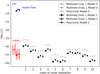Fig. B.1. Comparison of sampler outputs. Black points correspond to the evidence of the joint analysis (Model 0), while grey points correspond to split analysis (Model 1) for ten noise realisations measured from the traditional or importance-sampled approaches of MULTINEST, as well as from POLYCHORD. Red points display the mean and standard deviation over these realisations. Blue points show results for a noise-free data vector.

The χ² minimisation for the approximate method was performed with the built-in MONTE PYTHON maximum likelihood determination, with a precision tolerance of 10⁻⁹ on the log-likelihood. With this setup, a minimisation run consumes about 500 times less wall-clock time than full, parallelised sampling on high-performance computing infrastructure.

All Figures

Fig. 1. Illustration of model comparison via evidence and of its associated scatter for a one-dimensional data vector d and two models, Mi with i = 1, 2, each with a single parameter p. The joint distributions Pr(d,p|Mi) are shown in blue and red shades. The projections of these distributions onto the parameter and data axes yield the prior Pr(p|Mi) and the evidence or marginal likelihood, respectively (shown in purple and orange for M1 and M2). An experiment produces the observation d, shown as the solid black line. Conditioning on d yields the posterior Pr(p|d,Mi), shown in green and brown for M1 and M2. Evaluating the marginal likelihood at d yields Pr(d|Mi), which is used in the model comparison. The dotted horizontal lines mark the 1σ interval of possible alternative realisations of the data given the best-fit parameter pbest (dashed vertical lines) of either model. The blue and red boxes show the resulting 1σ range in possible evidence values under M1, which has higher evidence in this case (the corresponding ranges for M2 are shown as hatched areas).

In the text

Fig. 2. Joint distribution of the evidence calculated under two models (the mock KiDS cosmology analysis for a joint [Model 0] and a split [Model 1] data vector). The arrow indicates the direction of the increasing Bayes factor, lnR01, with the red line marking the true value of R01. Black points correspond to the inferences from 100 noise realisations of the mock data vector, evaluated on the full nested sampling analysis, and the blue points correspond to the ${\chi }_{\text{min}}^2$ approximation from Sect. 3. Contours show the Gaussian kernel density approximation of the distribution based on the black points.

In the text

Fig. 3. Probability density of the Bayes factor, lnR01, shifted to have its true value at 0. The black curve is the distribution of ΔlnR01 extracted from the full nested sampling analysis, and the blue curve is the distribution extracted from the ${\chi }_{\text{min}}^2$ approximation from Sect. 3. The green curve corresponds to the highly discrepant case of one of four tomographic redshift bins being shifted by dz = 0.3. Dotted lines mark the mean of each distribution.

In the text

Fig. 4. Tension statistics for the case of KiDS-450 internal consistency with respect to tomographic bin no. 3. Shown are the Bayes factor lnR01, with odds ratios, as well as the suspiciousness lnS01, with tension significance, in multiples of the width of an equivalent Gaussian, σ. The smaller red and black error bars are the errors associated with the nested sampling, while the larger orange and grey error bars are the statistical errors derived in this work. Red bands show the statistical uncertainty in determining the σ-levels for lnS01.

In the text

Fig. B.1. Comparison of sampler outputs. Black points correspond to the evidence of the joint analysis (Model 0), while grey points correspond to split analysis (Model 1) for ten noise realisations measured from the traditional or importance-sampled approaches of MULTINEST, as well as from POLYCHORD. Red points display the mean and standard deviation over these realisations. Blue points show results for a noise-free data vector.

In the text

References

- Abbott, T. M. C., Abdalla, F. B., Alarcon, A., et al. 2018, Phys. Rev. D, 98, 043526 [Google Scholar]
- Adhikari, S., & Huterer, D. 2019, J. Cosmol. Astropart. Phys., 2019, 036 [Google Scholar]
- Asgari, M., Tröster, T., Heymans, C., et al. 2020, A&A, 634, A127 [NASA ADS] [CrossRef] [EDP Sciences] [Google Scholar]
- Audren, B., Lesgourgues, J., Benabed, K., & Prunet, S. 2013, J. Cosmol. Astropart. Phys., 2013, 001 [NASA ADS] [CrossRef] [Google Scholar]
- Brinckmann, T., & Lesgourgues, J. 2019, Phys. Dark Univ., 24, 100260 [Google Scholar]
- Charnock, T., Battye, R. A., & Moss, A. 2017, Phys. Rev. D, 95, 123535 [NASA ADS] [CrossRef] [Google Scholar]
- Feroz, F., & Hobson, M. P. 2008, MNRAS, 384, 449 [NASA ADS] [CrossRef] [Google Scholar]
- Feroz, F., Hobson, M. P., & Bridges, M. 2009, MNRAS, 398, 1601 [NASA ADS] [CrossRef] [Google Scholar]
- Feroz, F., Hobson, M. P., Cameron, E., & Pettitt, A. N. 2019, Open J. Astrophys., 2, 10 [Google Scholar]
- Gelman, A., Meng, X.-L., & Stern, H. 1996, Stat. Sin., 6, 733 [Google Scholar]
- Good, I. J. 1992, J. Am. Stat. Assoc., 87, 597 [Google Scholar]
- Handley, W., & Lemos, P. 2019a, Phys. Rev. D, 100, 023512 [Google Scholar]
- Handley, W., & Lemos, P. 2019b, Phys. Rev. D, 100, 043504 [Google Scholar]
- Handley, W. J., Hobson, M. P., & Lasenby, A. N. 2015a, MNRAS, 450, L61 [Google Scholar]
- Handley, W. J., Hobson, M. P., & Lasenby, A. N. 2015b, MNRAS, 453, 4384 [NASA ADS] [CrossRef] [Google Scholar]
- Heavens, A. F., Jimenez, R., & Lahav, O. 2000, MNRAS, 317, 965 [NASA ADS] [CrossRef] [Google Scholar]
- Heavens, A. F., Kitching, T. D., & Verde, L. 2007, MNRAS, 380, 1029 [NASA ADS] [CrossRef] [Google Scholar]
- Heymans, C., Tröster, T., Asgari, M., et al. 2021, A&A, 646, A140 [NASA ADS] [CrossRef] [EDP Sciences] [Google Scholar]
- Hildebrandt, H., Viola, M., Heymans, C., et al. 2017, MNRAS, 465, 1454 [Google Scholar]
- Jaffe, A. 1996, ApJ, 471, 24 [NASA ADS] [CrossRef] [Google Scholar]
- Jenkins, C. 2014, Am. Inst. Phys. Conf. Ser., 1636, 106 [NASA ADS] [Google Scholar]
- Jenkins, C. R., & Peacock, J. A. 2011, MNRAS, 413, 2895 [NASA ADS] [CrossRef] [Google Scholar]
- Joudaki, S., Blake, C., Heymans, C., et al. 2017, MNRAS, 465, 2033 [NASA ADS] [CrossRef] [Google Scholar]
- Joudaki, S., Hildebrandt, H., Traykova, D., et al. 2020, A&A, 638, L1 [CrossRef] [EDP Sciences] [Google Scholar]
- Kass, R. E., & Raftery, A. E. 1995, J. Am. Stat. Assoc., 90, 773 [CrossRef] [Google Scholar]
- Köhlinger, F., Joachimi, B., Asgari, M., et al. 2019, MNRAS, 484, 3126 [NASA ADS] [Google Scholar]
- Kosowsky, A., Milosavljevic, M., & Jimenez, R. 2002, Phys. Rev. D, 66, 063007 [Google Scholar]
- Kuijken, K., Heymans, C., Hildebrandt, H., et al. 2015, MNRAS, 454, 3500 [Google Scholar]
- Kullback, S., & Leibler, R. A. 1951, Ann. Math. Statist., 22, 79 [CrossRef] [MathSciNet] [Google Scholar]
- Kunz, M., Trotta, R., & Parkinson, D. R. 2006, Phys. Rev. D, 74, 023503 [Google Scholar]
- Lazarides, G., Ruiz de Austri, R., & Trotta, R. 2004, Phys. Rev. D, 70, 123527 [NASA ADS] [CrossRef] [Google Scholar]
- Lemos, P., Köhlinger, F., Handley, W., et al. 2020, MNRAS, 496, 4647 [Google Scholar]
- Lin, W., & Ishak, M. 2017, Phys. Rev. D, 96, 023532 [NASA ADS] [CrossRef] [Google Scholar]
- MacKay, D. J. C. 2003, Information Theory, Inference and Learning Algorithms (Cambridge University Press) [Google Scholar]
- Marshall, P., Rajguru, N., & Slosar, A. 2006, Phys. Rev. D, 73, 067302 [NASA ADS] [CrossRef] [Google Scholar]
- Nicola, A., Amara, A., & Refregier, A. 2019, J. Cosmol. Astropart. Phys., 2019, 011 [Google Scholar]
- Petersen, K. B., & Pedersen, M. S. 2012, The Matrix Cookbook, version 20121115 [Google Scholar]
- Planck Collaboration V. 2020, A&A, 641, A5 [CrossRef] [EDP Sciences] [Google Scholar]
- Planck Collaboration VI. 2020, A&A, 641, A6 [NASA ADS] [CrossRef] [EDP Sciences] [Google Scholar]
- Prince, H., & Dunkley, J. 2019, Phys. Rev. D, 100, 083502 [NASA ADS] [CrossRef] [Google Scholar]
- Raveri, M., & Hu, W. 2019, Phys. Rev. D, 99, 043506 [Google Scholar]
- Riess, A. G., Macri, L. M., Hoffmann, S. L., et al. 2016, ApJ, 826, 56 [NASA ADS] [CrossRef] [Google Scholar]
- Riess, A. G., Casertano, S., Yuan, W., et al. 2018, ApJ, 861, 126 [NASA ADS] [CrossRef] [Google Scholar]
- Riess, A. G., Casertano, S., Yuan, W., Macri, L. M., & Scolnic, D. 2019, ApJ, 876, 85 [Google Scholar]
- Schuhmann, R. L., Joachimi, B., & Peiris, H. V. 2016, MNRAS, 459, 1916 [NASA ADS] [CrossRef] [Google Scholar]
- Seehars, S., Amara, A., Refregier, A., Paranjape, A., & Akeret, J. 2014, Phys. Rev. D, 90, 023533 [NASA ADS] [CrossRef] [Google Scholar]
- Skilling, J. 2006, Bayesian Anal., 1, 833 [Google Scholar]
- Tegmark, M., Taylor, A. N., & Heavens, A. F. 1997, ApJ, 480, 22 [NASA ADS] [CrossRef] [Google Scholar]
- Trotta, R. 2007, MNRAS, 378, 819 [NASA ADS] [CrossRef] [Google Scholar]
- Trotta, R. 2008, Contemp. Phys., 49, 71 [Google Scholar]
- Verde, L., Protopapas, P., & Jimenez, R. 2013, Phys. Dark Univ., 2, 166 [Google Scholar]
- Verde, L., Treu, T., & Riess, A. G. 2019, Nat. Astron., 3, 891 [Google Scholar]
- Wong, K. C., Suyu, S. H., Chen, G. C. F., et al. 2020, MNRAS, 498, 1420 [Google Scholar]