| Issue |
A&A
Volume 647, March 2021
|
|
|---|---|---|
| Article Number | A196 | |
| Number of page(s) | 8 | |
| Section | Cosmology (including clusters of galaxies) | |
| DOI | https://doi.org/10.1051/0004-6361/202039257 | |
| Published online | 05 April 2021 | |
An algorithm to locate the centers of baryon acoustic oscillations
Department of Physics and Astronomy, University of Rochester, 500 Joseph C. Wilson Boulevard, Rochester, NY 14627, USA
e-mail: zbrown5@ur.rochester.edu
Received:
25
August
2020
Accepted:
4
February
2021
Context. The cosmic structure formed from baryon acoustic oscillations (BAO) in the early universe is imprinted in the galaxy distribution observable in large-scale surveys and is used as a standard ruler in contemporary cosmology. Typically, BAOs are detected as a preferential length scale in two-point statistics, which gives little information about the location of the BAO structures in real space.
Aims. The aim of the algorithm described in this paper is to find probable centers of BAOs in the cosmic matter distribution.
Methods. The algorithm convolves the three-dimensional distribution of matter density with a spherical shell kernel of variable radius placed at different locations. The locations that correspond to the highest values of the convolution correspond to the probable centers of BAOs. This method is realized in an open-source, computationally efficient algorithm.
Results. We describe the algorithm and present the results of applying it to the SDSS DR9 CMASS survey and associated mock catalogs.
Conclusions. A detailed performance study demonstrates the ability of the algorithm to locate BAO centers and in doing so presents a novel detection of the BAO scale in galaxy surveys.
Key words: cosmology: observations / large-scale structure of Universe / dark matter / dark energy
© ESO 2021
1. Introduction
Baryon acoustic oscillations (BAOs) are density waves formed in the photon-baryon plasma in the primordial universe (Sunyaev & Zeldovich 1970; Peebles 1973; Eisenstein & Hu 1998; Bassett & Hlozek 2010). These oscillations are the result of the competition between the gravitational attraction pulling matter (mostly dark matter) into regions of high local density and radiation pressure pushing baryonic matter away from regions of high density. The resulting density waves, propagating at the sound speed of the plasma, produce “bubbles” with high-density centers, relatively underdense interiors, and overdense spherical “shells”. At the time of recombination when photons and matter fell out of thermal equilibrium, the bubbles are frozen into the matter distribution, with the centers remaining enriched in dark matter and shells enriched in baryonic matter (Eisenstein et al. 2007; Tansella 2018). After recombination the BAO centers and shells became the seeds of galaxy formation.
At late times the BAOs can be observed as a preferred length scale in the distribution of galaxies using the two-point correlation function (2pcf) and its Fourier transform, the power spectrum (Eisenstein et al. 2005; Percival et al. 2007) along with the three-point correlation function (3pcf) and its Fourier transform, the bispectrum (Slepian et al. 2017a,b). Since the BAO signal is a small perturbation in the large-scale clustering of galaxies, it is observed on a statistical basis. The positions of individual BAO centers and shells are not typically identified in large galaxy surveys. However, the identification of BAO centers would be of significant cosmological and astrophysical interest. For example, the cross-correlations between BAO centers and other tracers of large-scale structure, such as galaxies, voids, and dark matter tracers found via weak lensing, could probe different models of structure formation and provide sensitivity to deviations of primordial density fluctuations from Gaussian distribution, so-called non-Gaussianity.
The construction of higher-order correlation functions is computationally expensive, so we propose a method called CenterFinder1 to locate the centers of BAO bubbles and number of galaxies N displaced from the center by a distance RBAO. The CenterFinder algorithm is inspired by a template track-finding algorithm originally suggested in Hough (1962) and generalized in Ballard (1981), which is typically used in particle physics (see, e.g., Demina et al. 2004). In the following section, we describe the design and free parameters of the CenterFinder algorithm. In Sect. 3 we study the performance of CenterFinder using mock galaxy catalogs and the SDSS DR9 CMASS galaxy survey. We discuss the results in Sect. 4 and conclude in Sect. 5.
2. CenterFinder algorithm
CenterFinder locates BAO clustering centers by convolving three-dimensional spherical kernels of adjustable radii with tracers of large-scale structure. In this section we describe the inputs to the algorithm (Sect. 2.1), the estimator of the local density field (Sect. 2.2), the definition of the kernel (Sect. 2.3), the convolution step (Sect. 2.4), and the output (Sect. 2.5).
2.1. Input and coordinates
CenterFinder takes as its input catalogs of various matter tracers from surveys or simulations. For each tracer, its right ascension, αg, declination, δg, and redshift, zg, are required. Tracer weights, wg, may be used, but are not essential. Within the algorithm, celestial coordinates are converted to three-dimensional Cartesian coordinates. The relationship between the redshift and the comoving radial distance, rg, depends on the assumed cosmology, that is,
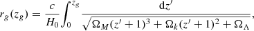
where ΩM, Ωk, and ΩΛ are the present-day values of the relative densities of dark matter, spatial curvature, and dark energy, respectively. The quantity H0 is the present day Hubble’s constant and c is the speed of light. The integral in Eq. (1) is evaluated numerically in CenterFinder. The Cartesian coordinates of each tracer are then evaluated according to
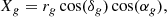
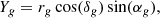
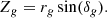
To prevent confusion with the redshift, z, Cartesian coordinates are given as capital letters, X, Y, Z.
2.2. Density field
Several methods of estimating the density field may be used in this algorithm. The details are provided in the associated README document. These methods rely on either raw or weighted galaxy histograms as well as the galaxy over-density with respect to the survey mean density. In this work we describe the option that is realized in this study. We start by defining a grid with spacing dc, such that the volume of each grid cell is  . The quantities Xi, Yj, Zk denote the Cartesian coordinates of the i, j, kth cell. On this grid we define three-dimensional histograms Nwtd(Xi, Yj, Zk), which denote a number count of tracers, and R(Xi, Yj, Zk), which represents a number count of randomly distributed points within the same fiducial volume as follows:
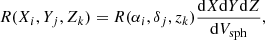
where dXdYdZ and dVsph give the volume of a particular cell in Cartesian and spherical sky coordinates. The distribution R(αi, δj, zk) is inferred from the input tracer catalog and is generated by assuming that the tracers’ angular, Pang(αi, δj), and redshift, Pz(zk), probability density distributions are factorizable (Demina et al. 2018) as follows:
![$$ \begin{aligned} R(\alpha _i,\delta _j,z_k) = N_{\rm tot} [ P_{\rm ang}(\alpha _i,\delta _j) \times P_z(z_k) ] , \end{aligned} $$](/articles/aa/full_html/2021/03/aa39257-20/aa39257-20-eq7.gif)
where Ntot is the number of tracers in the input catalog. If weights are available in the input catalogs, both Nwtd and R could be weighted. A three-dimensional local density difference histogram M(Xi, Yj, Zk) is then defined on the grid to represent the difference in density between Nwtd and R as follows:

2.3. Kernel
To probe for BAO bubbles, we begin by creating a spherical kernel, K(Xi, Yj, Zk), or a template to roughly model the distribution of matter expected around BAO centers, given a hypothesized BAO scale, R0. The kernel is constructed on a cube of the size of 2R0 in all directions, just large enough to encompass a sphere of radius R0. The grid defined on this cube has the same spacing, dc, as the grid used to construct M(Xi, Yj, Zk). Grid cells intersected by a sphere of radius R0 centered on the center of the cube are assigned a value of 1. All other cells are 0.
2.4. Convolution step
At this step we construct a three-dimensional histogram C(Xi, Yj, Zk), with entries that quantify the likelihood that a particular point in space (Xi, Yj, Zk) hosts a BAO center. The kernel K is first centered on some cell i, j, k and the value of C(Xi, Yj, Zk) is calculated as the scalar product of the kernel and the density map M. The kernel is then moved to a new cell and the process is repeated until the whole surveyed volume is covered. Thus, C(Xi, Yj, Zk) is a result of the convolution of the matter density map M with the kernel, K,

where * * * denotes a three-dimensional discrete convolution. One step in this process is visualized in Fig. 1.
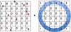 |
Fig. 1. Two-dimensional representation of the tracer density histogram (left), being convolved with the spherical kernel (right). In this example the tensor product is 7. |
If the original density histogram were the raw count of tracers, the value of C would have a simple meaning: it gives the number of tracers “voting” for a particular cell to host a center. A larger number of voters indicates a higher likelihood of a BAO center. While C does not directly correspond to voters when using the density estimate in Eq. (7), large values of C still correspond to increased likelihood of hosting a BAO center at a particular location.
This highly vectorized convolutional algorithm, called CenterFinder, is quite efficient; the runtime is set by the number of cells in the surveyed volume, which is in turn set by the one-dimensional grid length. Shown in Fig. 2, the runtime decreases with the grid length until it saturates at around 5 s. Prior to the saturation, the runtime scales as a power law, approximately  In our performance study (Sect. 3), a grid length of dc = 5.25 h−1 Mpc yields a runtime of approximately 240 s. This study applies CenterFinder to the northern Galactic cap (NGC) catalog of the SDSS DR9 CMASS survey using a personal computer with a 2.3 GHz Intel Core i7 processor and 8 GB of memory.
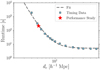 |
Fig. 2. Runtime of CenterFinder, given as a function of the grid length, for one of the CMASS mocks used in this study (blue squares). The red star indicates the value of dc chosen in this analysis. The timing data is fit to a log power law of the form A(dc/dscale)α + βlog(dc/dscale) + C (dashed gray line). In the above fit, the value of the parameter α is approximately −5. |
2.5. Output
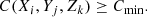
Once the three-dimensional histogram C is generated, it is converted into a catalog of probable BAO centers by applying a user-specified threshold, Cmin, on C as follows:
The output catalog in astropy FITS format provides the locations (right ascensions, declinations, and redshifts) of the probable centers and weights corresponding to the values of C. The redshifts are calculated using the inverse of the relation in Eq. (1). Redshifts, rather than radial distances, are included since most algorithms for probing cosmological structure are designed to be applied to redshift catalogs.
3. Performance study
3.1. Galaxy survey data, mock catalogs, and random catalogs
The performance of CenterFinder, that is, its ability to locate BAO centers, is tested on the SDSS DR9 CMASS galaxy survey (Ahn et al. 2012; Padmanabhan et al. 2012) and on an ensemble of associated mock and random catalogs. We limit our analysis to galaxies in the north Galactic cap of the survey. Details regarding the mock catalogs may be found in Manera et al. (2013). The mock ensemble consists of 20 catalogs. The random ensemble also consists of 20 catalogs of density equal to that of the mocks, appropriately sampled from the several large random catalogs.
3.2. Cosmology and the two-point correlation function
In this study we used the following values for cosmological parameters: c = 300 000 km s−1, H0 = 100 h km s−1 Mpc−1, ΩM = 0.274, ΩΛ = 0.726, and Ωk = 0. Before analyzing the catalogs with CenterFinder, we investigated the clustering behavior of the DR9 galaxies and mocks with the 2pcf, ξ(s). We compute ξ(s) using the estimator of Landy and Szalay (Landy & Szalay 1993; Hamilton 1993),
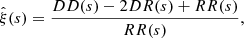
where DD, RR, and DR are the normalized distributions of the pairwise combinations of galaxies from “data”, D, and “random”, R, catalogs (plus cross terms) at given distances s from one another. The 2pcf calculations are done using the algorithm described in Demina et al. (2018).
The 2pcf calculated using bin width Δs = 2.5 h−1 Mpc is shown for data and mocks in Fig. 3. In both catalogs there is evidence of clustering at small scales and a prominent BAO signal around 109 h−1 Mpc, which is consistent with previous analyses on the same data sets (Anderson et al. 2012; Ross et al. 2012). We note that both at small scales and near the BAO scale, the magnitude of  is noticeably smaller in the average over mocks compared to the DR9 survey data. Additionally, the variance between mocks in this ensemble is considerable at separations approaching the BAO scale.
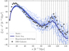 |
Fig. 3. Two-point correlation function, |

3.3. CenterFinder procedure
To identify a BAO signal using CenterFinder, we apply it to SDSS DR9 CMASS data, mock, and random catalogs. Random catalogs match the fiducial volume and the galaxy density of the survey. The cosmology used is identical to that used in the calculation of the 2pcf.
We generated a density map M using the method described in Sect. 2.2, with a grid spacing, dc = 5.25 h−1 Mpc. When generating the density field, we keep only cells with positive values because our tracers, galaxies, indicate regions of over density. The radius of the kernel, R0, is varied from 80.5 to 139 h−1 Mpc in 4.9 h−1 Mpc steps. For each value of R0, the kernel is convolved with the density map M to generate a map of weights, C(R0), where larger values indicate a higher probability of BAO centers being present at that location in space. The distribution of the values of C(R0) from a random catalog is shown in Fig. 4 for different kernel sizes.
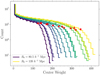 |
Fig. 4. Distribution of center weights, for kernels of different sizes, applied to a random catalog with the same fiducial volume and density as the SDSS DR9 CMASS NGC survey. The dark blue curve corresponds to R0 = 80.5 h−1 Mpc and yellow corresponds to R0 = 139 h−1 Mpc. Intermediate colors correspond to the intermediate kernel sizes used in this analysis. The red stars indicate the threshold values, Cmin used to create catalogs of probable centers at each kernel size. |
These distributions have three prominent features. First, the vast majority of cells in the grid are empty or nearly empty, and their convolution with the kernel yields small values of C, as shown by the sharp spike at low weights. This is followed by gradual falling off, which extends to higher values for larger kernels. Finally, there is a sharp drop in counts as the weights increase.
To reduce the size of the output catalog we keep only the cells with values larger than a certain threshold, Cmin, which is chosen to keep the count of centers approximately constant for different values of R0. Since the number of counts on a spherical shell is proportional to the radius squared, we expect Cmin to be approximately proportional to  . We choose values of Cmin (shown by red stars in Fig. 4), which correspond to the beginning of a sharp drop off. We apply a threshold selection at Cmin = 150 for the smallest kernel size and at Cmin = 300 for the largest. The dependence of the chosen thresholds on the kernel size shown in Fig. 5. As expected, this dependence is well fit by the second order polynomial.
 |
Fig. 5. Threshold values, Cmin, applied to our center catalogs, as a function of the kernel size (blue squares). The points are fit to a second order polynomial (dashed grey line). |
Finally, we generate FITS catalogs of the probable centers based on 20 mock, 20 random, and DR9 data catalogs for several values of the kernel size.
3.4. Illustration of CenterFinder
Using a sample of galaxies from the SDSS DR9 survey as an example, we illustrate the output of CenterFinder. In Fig. 6 we show a slice in the redshift region from z = 0.51 to z = 0.52 from the catalog of probable centers generated using the kernel size of R0 = 109.9 h−1 Mpc. The color of the background represents the weights C, which characterize the probability that a particular point is a location of a BAO center with more intense yellow being the most probable. The red points show the location of the galaxies from the SDSS DR9 catalog from the same fiducial volume. The dashed lines are circles of 109.9 h−1 Mpc radius around the probable BAO centers. Even in this two-dimensional slice, we observe significant overlap between the circles denoting the BAO shells and the galaxies from the survey. Since we chose a fairly low value for the threshold selection of BAO centers, there are multiple circles around the same location with high probability to host the BAO center. It is also noticeable that these locations typically host several galaxies, supporting the hypothesis that dark matter enriched BAO centers are likely to be seeds for galaxy formation.
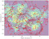 |
Fig. 6. Angular distribution of the probable centers for the redshift range 0.51 < z < 0.52 (color scale), generated from the R0 = 109.9 h−1 Mpc kernel on a portion of the SDSS DR9 data. Galaxies locations are shown as red stars. The dashed circles reflect the angles subtended by the BAO spheres at z = 0.515. BAO circles are only shown around the most probable center locations. |
3.5. Probable center to galaxy cross correlations
Since potential centers correspond to primordial over-dense regions, we expect the galaxies to have been preferentially formed in these regions of space. We test this hypothesis by cross correlating the potential BAO centers, DC, with galaxies, DG, drawn from data or mock catalogs. For each catalog of centers, generated using a kernel of size R0, we calculate a cross-correlation function,  given by
where RC and RG are random catalogs corresponding to the center and galaxy catalogs, respectively. All pairwise distributions are functions of the distance between a center and a galaxy, s and the hypothesized BAO scale, R0.
The catalog RG corresponds to the random galaxies used in the evaluation of the 2pcf (Sect. 3.2); RC is a catalog of NCR randomly distributed centers. The ratio of NCR to the number of found centers is chosen to be similar to the ratio of the number of galaxies in data D to the size of the random catalog R. We generate RC by applying CenterFinder to several random galaxy catalogs. The angular and redshift distributions of RC match those of the probable centers, DC, as detailed in in Appendix A.
The quantity  is evaluated using nbodykit, which is described in Hand et al. (2018). Figures 7–9 show the result of the center-galaxy cross correlation in data, mock, and random catalogs, respectively. The distributions are divided into s bins of width Δs = 3.8 h−1 Mpc and R0 bins reflecting the sampling when applying CenterFinder.
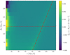 |
Fig. 7. Cross correlation of probable center locations with SDSS DR9 galaxies as a function of the objects’ separation, s, and the hypothesized BAO scale of CenterFinder used to generate the center catalog, R0. The cross correlation is adjusted for clarity (divided by s). The dashed line (red) indicates an estimate of the BAO scale observed in the 2pcf. The dot-dashed line (red) indicates s = R0. |
Two clustering features are present in Figs. 7 and 8. First, a region of higher values of  , which follows s = R0 is observed in both plots, with roughly equal magnitude across mock and SDSS DR9 data. This feature is an artifact of the CenterFinder. The algorithm is designed to find centers of densely populated spherical shells of a given radius. The observed excess is simply the correlation between the galaxies in these shells with the corresponding found centers. This feature confirms the most basic function of the algorithm, but is not physically informative.
The second feature in both mock and DR9 survey data is the observed increase in  at low s, which is enhanced when the hypothized BAO radius is near the true BAO scale (horizontal dashed line) (Anderson et al. 2012; Ross et al. 2012) and diminished at larger and smaller radii. This behavior confirms our original hypothesis that galaxies cluster around the potential BAO centers. The first (diagonal) feature corresponding to the kernel radius is observed in random catalogs (Fig. 9), but there is no excess at the small scales. This qualitatively confirms that the signal at low s seen in the mocks and in the data is due to large-scale structures and is not a random fluctuation.
We note that the BAO signal (increase in  at low s) is larger in magnitude for SDSS DR9 data (Fig. 7) compared to the average over the mock catalogs (Fig. 8). This is consistent with the fact that the mock catalogs showed on average less overall galaxy clustering in the 2pcf than the SDSS DR9 data (Fig. 3). This is also observed in the distribution of probable center weights, C, shown in Fig. 10. The distribution in Fig. 10 are shown prior to applying a threshold, Cmin.
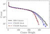 |
Fig. 10. Distribution of center weights, for a kernel with a radius reflecting the approximate BAO scale, extracted from the 2pcf, R0 = 109.9 h−1 Mpc for SDSS DR9 galaxies (solid black line), one of the CMASS mocks (blue dashed line), and one of the CMASS randoms (dot-dashed red line). The shaded regions represent uncertainties across a range of values for ΩM, which is equal to the uncertainty in the most recent estimate from the Planck Collaboration. |
The SDSS DR9 galaxies show higher counts of probable centers with larger weights or values of C. This suggests a higher degree of galaxy density and clustering on the BAO shells. This observation is consistent with the increased clustering behavior seen in the 2pcf. Furthermore, the distributions of probable center weights in Fig. 10 show that the SDSS DR9 galaxies and CMASS mock significantly deviate from the distribution extracted from randoms at large weights. This indicates the presence of BAO shells imprinted in the mock and data galaxy distributions.
3.6. Quantifying the BAO signal
To quantify the strength of the presumed BAO signal we sum the values of  in the first ten s-bins (from s = 3.72 to s = 42.2 h−1 Mpc) for every R0 value. The results are shown in Fig. 11 for the SDSS DR9 data, mock, and random catalogs. The distribution over signal strengths for mocks and randoms, as well as the value for SDSS DR9 data at R0 = 109.9 h−1 Mpc, is shown in Fig. 12. There is a large spread in signal strength for the mocks at every kernel size, which is in agreement with the behavior observed in the two-point statistics (Fig. 3). The signal strength derived from random catalogs, on the other hand, is centered around 0 and shows a much smaller spread. At the kernel size corresponding to the BAO scale, R0 = 109.9 h−1 Mpc, we find that the SDSS DR9 data differ from the mean of the CMASS randoms by 5.0 standard deviations excluding the probability of a random fluctuation at more than 99% CL.
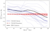 |
Fig. 11. Signal strength as a function of kernel size. Each mock is shown individually (blue), as is DR9 data (black), while randoms (red) are represented by a mean of all values at each kernel size, with a shaded region given by the standard deviations. |
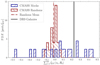 |
Fig. 12. Normalized histogram of the signal strengths at R0 = 109.9 h−1 Mpc for the CMASS randoms (red) and CMASS mocks (blue). The SDSS DR9 data (black) are shown as a vertical line at 0.224, 5.0 standard deviations away from the random mean at −0.015. |
3.7. Sensitivity to fiducial cosmology
We evaluate the sensitivity of the algorithm to the cosmological parameters used to convert from celestial to Cartesian coordinates in Eq. (1). The explicit sensitivity to H0 is removed by presenting all distances in units of h−1 Mpc. Sensitivity to flat ΛCDM parameters was evaluated by varying the value of ΩM from that used to generate CMASS mock catalogs within the uncertainties corresponding to that of the most recent measurement by Planck Collaboration (Planck Collaboration VI 2020): ΩM = 0.274 ± 0.007. The corresponding variation in the center weights is shown by the shading in Fig. 10. Based on this study, we conclude that the observed signal has negligible dependence on the choice of fiducial cosmology.
4. Discussion
From the geometrical point of view, the problem that is solved by the CenterFinder can be reduced to an image (in this case a sphere) recognition in a high noise environment. Different machine learning techniques have been successfully employed to solve similar problems (see, e.g., Kim & Brunner 2017). However, CenterFinder produces results without added levels of abstraction associated with machine learning approaches. The output of the CenterFinder (e.g., the center weights) can be easily interpreted and, for this reason, can be used to distinguish between cosmological models. At the same time, to improve the signal-to-noise ratio, this output can be used to feed into the training of a neural network.
An approach similar to this work was suggested in Arnalte-Mur et al. (2012), where a more complex kernel shape was used emulating a spherical wavelet template. Our algorithm also allows for the use of different kernel shapes, including a similarly shaped wavelet. Another difference is that CenterFinder scans over the entire surveyed volume identifying BAO centers that may or may not be associated with other galaxies, while the algorithm described in Arnalte-Mur et al. (2012) uses luminous red galaxies as seeds to search for spherical shells. Hence the output of CenterFinder can be cross correlated with other matter tracers, such as Lyman-α forest and dark matter maps generated using weak lensing.
We note that the catalogs of probable BAO centers in real space may be used as a cosmological probe. As our performance study demonstrates the cross correlation between the found centers and the original matter tracers is sensitive to the BAO scale. Cosmological parameters, most notably the Hubble constant H0, are constrained by the measured BAO scale. This paper presents a proof of principle for the center finding technique. When generating catalogs of probable BAO centers, we apply a threshold (Sect. 2.5), which in this study, was defined manually. This threshold, as well as other algorithm parameters, can be optimized to provide the optimal precision in the definition of the BAO scale.
While CenterFinder provides a novel way to determine the BAO scale, the precision of such measurement is unlikely to surpass that of the standard techniques such as a 2pcf or the power spectrum (see, e.g., Cuceu et al. 2019). However, it was pointed out that higher order statistics, such as 3pcf and bispectrum, are particularly important in constraining primordial non-Gaussianities (Desjacques & Seljak 2010). CenterFinder, which also probes the higher order correlations in the density field perturbations, is also expected to be able to probe for non-Gaussian fields. While quantitatively this statement will need to be verified through an application of CenterFinder to simulations of non-Gaussian random fields, qualitatively it can be understood via the following argument. Non-Gaussian fluctuations of the random fields will result in larger variations in the local density compared to Gaussian random fields. Centers with large local density would attract more baryonic matter, resulting in more densely populated shells. CenterFinder would identify such shells as having a higher center weight. Thus, the distributions of probable center weights shown in Fig. 10 is potentially sensitive to non-Gaussian fields. Moreover, matter clustering around the BAO center is also sensitive to the original deviation of the density field from the mean, and hence to non-Gaussianities. Different matter tracers can be used to characterize such clustering, such as galaxies, Lyman-α forest, and weak lensing, opening a rich field for multivariate analysis with a potential involvement of the machine learning techniques.
5. Conclusions
In this paper we present the algorithm CenterFinder designed to locate centers of spherical shells generated by BAOs. So far the BAO signature has been observed as a statistical feature in the CMB power spectrum and in the 2pcf of galaxy distributions. This algorithm is computationally efficient and can be applied to a variety of tracer catalogs. A performance study using SDSS DR9 survey and mock catalogs yielded a novel method to detect the BAO scale and to generate catalogs of probable BAO center locations to study in future analyses. Using these catalogs of centers, cross correlations between them and other tracers of the cosmic web such as clusters, voids, Lyman-α forest, and weak lensing maps may be studied.
The source code may be downloaded from https://github.com/mishtak00/centerfinder
Acknowledgments
The authors would like to thank S. BenZvi, K. Douglass and S. Gontcho A Gontcho for useful discussions and insightful questions. R. D. thanks D. Bianchi, L. Samushia and Z. Slepian for their interest and helpful comments. The authors acknowledge support from the Department of Energy under the grant DE-SC0008475.0. Funding for SDSS-III has been provided by the Alfred P. Sloan Foundation, the Participating Institutions, the National Science Foundation, and the US Department of Energy Office of Science. The SDSS-III web site is http://www.sdss3.org/. SDSS-III is managed by the Astrophysical Research Consortium for the Participating Institutions of the SDSS-III Collaboration including the University of Arizona, the Brazilian Participation Group, Brookhaven National Laboratory, Carnegie Mellon University, University of Florida, the French Participation Group, the German Participation Group, Harvard University, the Instituto de Astrofisica de Canarias, the Michigan State/Notre Dame/JINA Participation Group, Johns Hopkins University, Lawrence Berkeley National Laboratory, Max Planck Institute for Astrophysics, Max Planck Institute for Extraterrestrial Physics, New Mexico State University, New York University, Ohio State University, Pennsylvania State University, University of Portsmouth, Princeton University, the Spanish Participation Group, University of Tokyo, University of Utah, Vanderbilt University, University of Virginia, University of Washington, and Yale University.
References
- Ahn, C. P., Alexandroff, R., Prieto, C. A., et al. 2012, ApJS, 203, 21 [NASA ADS] [CrossRef] [Google Scholar]
- Anderson, L., Aubourg, E., Bailey, S., et al. 2012, MNRAS, 427, 3435 [Google Scholar]
- Arnalte-Mur, P., Labatie, A., Clerc, N., et al. 2012, A&A, 542, A34 [NASA ADS] [CrossRef] [EDP Sciences] [Google Scholar]
- Ballard, D. H. 1981, Pattern Recognit., 13, 111 [Google Scholar]
- Bassett, B., & Hlozek, R. 2010, Dark Energy: Observational and Theoretical Approaches,, 246 (Cambridge, UK: Cambridge University Press) [Google Scholar]
- Cuceu, A., Farr, J., Lemos, P., & Font-Ribera, A. 2019, JCAP, 2019, 044 [Google Scholar]
- Demina, R., Khanov, A., Rizatdinova, F., & Shabalina, E. 2004, DØ internal note [Google Scholar]
- Demina, R., Cheong, S., BenZvi, S., & Hindrichs, O. 2018, MNRAS, 480, 49 [NASA ADS] [CrossRef] [Google Scholar]
- Desjacques, V., & Seljak, U. 2010, CQG, 27 [Google Scholar]
- Eisenstein, D. J., & Hu, W. 1998, ApJ, 496, 605 [NASA ADS] [CrossRef] [Google Scholar]
- Eisenstein, D. J., Zehavi, I., Hogg, D. W., et al. 2005, ApJ, 633, 560 [Google Scholar]
- Eisenstein, D. J., Seo, H.-J., & White, M. 2007, ApJ, 664, 660 [NASA ADS] [CrossRef] [Google Scholar]
- Hamilton, A. J. S. 1993, ApJ, 417, 19 [NASA ADS] [CrossRef] [Google Scholar]
- Hand, N., Feng, Y., Beutler, F., et al. 2018, AJ, 156, 160 [Google Scholar]
- Hough, P. 1962, U.S. Patent, 3, 654 [Google Scholar]
- Kim, E. J., & Brunner, R. J. 2017, MNRAS, 464, 4463 [NASA ADS] [CrossRef] [Google Scholar]
- Landy, S. D., & Szalay, A. S. 1993, ApJ, 412, 64 [Google Scholar]
- Manera, M., Scoccimarro, R., Percival, W. J., et al. 2013, MNRAS, 428, 1036 [NASA ADS] [CrossRef] [Google Scholar]
- Padmanabhan, N., Xu, X., Eisenstein, D. J., et al. 2012, MNRAS, 427, 2132 [NASA ADS] [CrossRef] [MathSciNet] [Google Scholar]
- Peebles, P. 1973, ApJ, 185, 413 [NASA ADS] [CrossRef] [Google Scholar]
- Percival, W. J., Cole, S., Eisenstein, D. J., et al. 2007, MNRAS, 381, 1053 [NASA ADS] [CrossRef] [MathSciNet] [Google Scholar]
- Planck Collaboration VI. 2020, A&A, 641, A6 [NASA ADS] [CrossRef] [EDP Sciences] [Google Scholar]
- Ross, A. J., Percival, W. J., Sánchez, A. G., et al. 2012, MNRAS, 424, 564 [NASA ADS] [CrossRef] [Google Scholar]
- Slepian, Z., Eisenstein, D. J., Beutler, F., et al. 2017a, MNRAS, 468, 1070 [Google Scholar]
- Slepian, Z., Eisenstein, D. J., Brownstein, J. R., et al. 2017b, MNRAS, 469, 1738 [Google Scholar]
- Sunyaev, R. A., & Zeldovich, Y. B. 1970, Astrophys. Space Sci., 7, 3 [Google Scholar]
- Tansella, V. 2018, Phys. Rev. D, 97, 103520 [Google Scholar]
Appendix A: Galaxy, random, and center distributions
In Sect. 3.5, we cross correlate objects from two catalogs, galaxies and probable centers. In addition, the galaxies and probable BAO centers are compared to random distributions, RG and RC. In Figs. A.1 and A.2, we show the distributions of these tracers over their coordinates.
 |
Fig. A.1. Distribution over the right ascension (top), declination (middle), and redshift (bottom) for the SDSS DR9 CMASS galaxies (blue) and random galaxies (orange). |
 |
Fig. A.2. Distribution over the right ascension (top), declination (middle), and redshift (bottom) for the probable centers at R0 = 109.9 h−1 Mpc, generated from both data (green) and randoms (red). |
The probable centers are clearly biased toward regions of the survey with high galaxy density. While the method outlined in Sect. 2.2 corrects for some of this, Figs. A.1 and A.2 demonstrate that the effect is not entirely removed. The difference in the distribution over the redshift especially justifies the use of an additional random catalog, RC, in the evaluation of the galaxy to probable center cross correlation.
All Figures
|
Fig. 1. Two-dimensional representation of the tracer density histogram (left), being convolved with the spherical kernel (right). In this example the tensor product is 7. |
| In the text | |
|
Fig. 2. Runtime of CenterFinder, given as a function of the grid length, for one of the CMASS mocks used in this study (blue squares). The red star indicates the value of dc chosen in this analysis. The timing data is fit to a log power law of the form A(dc/dscale)α + βlog(dc/dscale) + C (dashed gray line). In the above fit, the value of the parameter α is approximately −5. |
| In the text | |
|
Fig. 3. Two-point correlation function, |
| In the text | |
|
Fig. 4. Distribution of center weights, for kernels of different sizes, applied to a random catalog with the same fiducial volume and density as the SDSS DR9 CMASS NGC survey. The dark blue curve corresponds to R0 = 80.5 h−1 Mpc and yellow corresponds to R0 = 139 h−1 Mpc. Intermediate colors correspond to the intermediate kernel sizes used in this analysis. The red stars indicate the threshold values, Cmin used to create catalogs of probable centers at each kernel size. |
| In the text | |
|
Fig. 5. Threshold values, Cmin, applied to our center catalogs, as a function of the kernel size (blue squares). The points are fit to a second order polynomial (dashed grey line). |
| In the text | |
|
Fig. 6. Angular distribution of the probable centers for the redshift range 0.51 < z < 0.52 (color scale), generated from the R0 = 109.9 h−1 Mpc kernel on a portion of the SDSS DR9 data. Galaxies locations are shown as red stars. The dashed circles reflect the angles subtended by the BAO spheres at z = 0.515. BAO circles are only shown around the most probable center locations. |
| In the text | |
|
Fig. 7. Cross correlation of probable center locations with SDSS DR9 galaxies as a function of the objects’ separation, s, and the hypothesized BAO scale of CenterFinder used to generate the center catalog, R0. The cross correlation is adjusted for clarity (divided by s). The dashed line (red) indicates an estimate of the BAO scale observed in the 2pcf. The dot-dashed line (red) indicates s = R0. |
| In the text | |
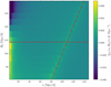 |
Fig. 8. Same as in Fig. 7 for mock galaxies. |
| In the text | |
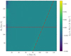 |
Fig. 9. Same as in Fig. 7 for random galaxies. |
| In the text | |
|
Fig. 10. Distribution of center weights, for a kernel with a radius reflecting the approximate BAO scale, extracted from the 2pcf, R0 = 109.9 h−1 Mpc for SDSS DR9 galaxies (solid black line), one of the CMASS mocks (blue dashed line), and one of the CMASS randoms (dot-dashed red line). The shaded regions represent uncertainties across a range of values for ΩM, which is equal to the uncertainty in the most recent estimate from the Planck Collaboration. |
| In the text | |
|
Fig. 11. Signal strength as a function of kernel size. Each mock is shown individually (blue), as is DR9 data (black), while randoms (red) are represented by a mean of all values at each kernel size, with a shaded region given by the standard deviations. |
| In the text | |
|
Fig. 12. Normalized histogram of the signal strengths at R0 = 109.9 h−1 Mpc for the CMASS randoms (red) and CMASS mocks (blue). The SDSS DR9 data (black) are shown as a vertical line at 0.224, 5.0 standard deviations away from the random mean at −0.015. |
| In the text | |
|
Fig. A.1. Distribution over the right ascension (top), declination (middle), and redshift (bottom) for the SDSS DR9 CMASS galaxies (blue) and random galaxies (orange). |
| In the text | |
|
Fig. A.2. Distribution over the right ascension (top), declination (middle), and redshift (bottom) for the probable centers at R0 = 109.9 h−1 Mpc, generated from both data (green) and randoms (red). |
| In the text | |
Current usage metrics show cumulative count of Article Views (full-text article views including HTML views, PDF and ePub downloads, according to the available data) and Abstracts Views on Vision4Press platform.
Data correspond to usage on the plateform after 2015. The current usage metrics is available 48-96 hours after online publication and is updated daily on week days.
Initial download of the metrics may take a while.