| Issue |
A&A
Volume 646, February 2021
|
|
|---|---|---|
| Article Number | A179 | |
| Number of page(s) | 6 | |
| Section | The Sun and the Heliosphere | |
| DOI | https://doi.org/10.1051/0004-6361/202039850 | |
| Published online | 23 February 2021 | |
Spatial quasi-periodic variations of the plasma density and magnetic field in zebra radio sources
1
Astronomical Institute of the Czech Academy of Sciences, Fričova 298, 251 65 Ondřejov, Czech Republic
e-mail: This email address is being protected from spambots. You need JavaScript enabled to view it.
2
St.-Petersburg State University, St.-Petersburg 198504, Russia
3
St.-Petersburg branch of Special Astrophysical Observatory, 196140 St.-Petersburg, Russia
Received:
5
November
2020
Accepted:
12
January
2021
Abstract
Context. Radio bursts and their fine structures are an integral part of solar flares. Fine structures in particular are used for diagnostics of solar flare processes. The so-called zebras belong to the most important of such fine structures.
Aims. We analyze seven zebra events in order to search for spatial variations in the plasma density and magnetic field in zebra-stripe sources.
Methods. We used an improved method for estimating the gyroharmonic numbers of zebra-stripe frequencies. We compared observed zebra-stripe frequencies with those calculated in the zebra model. The differences in these frequencies vary and thus show spatial variations in the plasma density and magnetic field.
Results. In six out of seven analyzed zebras, we found a rather high correlation coefficient (about 0.7 and higher) between spatial variations in the density and magnetic field and a strictly periodic function. These density and magnetic field variations are explained by the torsional or sausage magnetoacoustic waves in the loop in which zebra-stripe sources are located. We present the wavelengths of these waves in dependence on the zebra frequency and estimate their periods.
Key words: Sun: flares / Sun: radio radiation / Sun: oscillations
© ESO 2021
1. Introduction
Zebra patterns (ZP), or zebras for short, are observed in the form of regular stripes in emission in the dynamic radio spectrum. Their observational parameters have been presented in many reviews and monographs (Kuijpers 1975; Slottje 1981; Chernov 2006, 2011). The statistics and classification of microwave zebras have been reported by Tan et al. (2014). To date, more than ten mechanisms for generating ZP have been proposed. The most commonly discussed mechanism in the literature is the mechanism based on the double plasma resonance (DPR), in which the radiation is at the upper hybrid frequency and simultaneously at the electron cyclotron harmonics with the integer gyroharmonic number s (Kuijpers 1975, 1980; Zheleznyakov & Zlotnik 1975; Mollwo 1983, 1988; Winglee & Dulk 1986). A number of works have also been devoted to other mechanisms of ZP generation, see, for example, Chernov (1976, 1990), Karlický et al. (2001), LaBelle et al. (2003), Bárta & Karlický (2006), Ledenev et al. (2006), Kuznetsov & Tsap (2007) and Laptukhov & Chernov (2009).
Karlický (2014) interpreted the frequency variations of the zebra stripes as being caused by the plasma turbulence. These frequency variations were analyzed with the Fourier method, and power spectra with a power-law index close to the Kolmogorov index were found.
Karlický & Yasnov (2018) proposed a model of the zebra source in a plasma tube based on the double plasma resonance (DPR) mechanism. In this model, the density and magnetic field were expressed with exponential functions along the longitudinal and transversal coordinates of this tube. As shown in Karlický & Yasnov (2019), to generate isolated ZP stripes in this model, the following relation for dimensionless field and density scales (i.e., relative to the density scale along the tube radius r) has to be satisfied:
 (1)
(1)
where Lbr, Lbh, and Lnh are the magnetic field scales along the tube radius r and tube height h and the density scale along the height h, respectively.
When diagnosing physical conditions in the zebra sources, it is the most important to determine the value of the gyroharmonic number s, which corresponds to a specific zebra stripe in the time-frequency spectrum. Karlický & Yasnov (2015) and Yasnov & Karlický (2020) considered the DPR mechanism and developed a method and improved it for determining the gyroharmonic s, including the spatial variability of the magnetic field and density scales. Karlický & Yasnov (2019) derived a formula for the theoretical zebra-stripe frequency based on the theory of ZP with DPR mechanism as
 (2)
(2)
where s is the gyroharmonic number of the zebra stripe, f(s1) is the lowest stripe frequency with s = s1, and R = Lbh/Lnh =  is the ratio of the magnetic field and density scales.
Karlický & Yasnov (2020) showed that the observed zebra-stripe frequencies in the 14 February 1999 zebra event deviate from those in the model with DPR. These deviations were interpreted as being caused by a spatially varying turbulence in the zebra-stripe sources. The turbulence levels in the density and magnetic field related to this zebra event were therefore estimated.
In the present paper we extend the study of Karlický & Yasnov (2020) to more zebra events. Moreover, we use a more general approach to determine the gyroharmonic number of zebra stripes. That is, we use the linear dependance of R on the gyroharmonic number as presented in Yasnov & Karlický (2020), instead of R = constant used in Karlický & Yasnov (2020). Using this more general method, we recognize spatial quasi-periodic variations in zebra sources. These spatial variations are then discussed together with the quasi-periodic oscillations and waves that are frequently observed in solar flares (Nakariakov & Melnikov 2009; Tan et al. 2010; Nakariakov et al. 2016).
2. Zebra event analysis
2.1. 21 June 2011 zebra (Kaneda et al. 2018)
To determine the gyroharmonic numbers of the zebra stripes, we used the improved method described by Yasnov & Karlický (2020). For this method it is useful to rewrite the relation (2) as follows:
 (3)
(3)
where n = s1 − s + 1 is the ordinal number of the zebra stripes from the lowest to higher frequencies, that is, n = 1, n = 2, n = 3, and so on. In our method we fit the observed frequencies of zebra stripes with the model frequencies (relation 3). Here, the ratio R = Lbh/Lnh (where Lbh and Lnh are the spatial scales of the magnetic field and density in the region where a zebra is generated) is taken as linearly varying in space, that is, R = R1 + R2(n − 1) is the linear function of n, where R1 and R2 are constants. We note that in the DPR model, zebra-stripe sources are at different locations. Thus, n in R expresses the distances of zebra-stripe sources.
In the 21 June 2011 event we took the zebra-stripe frequencies from Kaneda et al. (2018) and assumed, as in Kaneda et al. (2018), that the zebra emission is generated by the DPR mechanism and is emitted at the first harmonic of the upper hybrid frequency. Using our fitting method, we then determined the parameters of ZP at 03:22:27.4 UT, when ZP was expressed the most distinctly. As a result, we obtained the ratio of the magnetic field and density scales along and across the axis of the tube-emitting region R = Lbh/Lnh = (Lbr/Lnr)2 = R1 + R2(n − 1) with R1 = 1.15 and R2 = 0.0028, and the gyroharmonic number s1 = 152 with the corresponding frequency f(s1) = 160.7 MHz. The ratio R > 1 means that the magnetic field scale Lbh is greater than the density scale Lnh. It differs from the solar atmosphere described by the mean magnetic field according to Dulk & McLean (1978), for example, and from the density according to the relation of Baumbach and Allen (Allen 1947), where Lnh is greater than Lbh. A positive value of R also indicates that the magnetic field and density gradients in the ZP source have the same negative sign.
Similarly as in Karlický & Yasnov (2020), we calculated the difference between the observed zebra-stripe frequencies fob and those fth calculated using Eq. (3). This difference in dependence on the zebra-stripe frequency for the zebra at 03:22:27.4 UT is shown in Fig. 1. The plot shows a quasi-periodic variation of fob − fth.
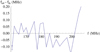 |
Fig. 1. Difference between the zebra-stripe frequencies fob observed at 03:22:27.4 UT and those fth calculated according to Eq. (3) in dependence on the zebra-stripe frequency. At the lowest frequency, the error bar is shown, calculated from the accuracy in determining the observed zebra-stripe frequencies. |
We calculated the relative variations in the magnetic field dB/B and plasma density dN/N in the zebra-stripe sources. For this purpose, we used the relations as follows:
 (4)
(4)
where fth(n) and fob(n) are the theoretically calculated and observed zebra-stripe frequencies, respectively. For comparison, we then approximated the relative density variations with a cosine function of amplitude A = 0.00064 and wavelength Lchar = 3.50. The results of these calculation together with the cosine approximation are shown in Fig. 2.
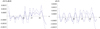 |
Fig. 2. Variations computed for the 21 June 2011 zebra at 03:22:27.4 UT. Left: relative variations in magnetic field dB/B (solid line) and plasma density dN/N (dashed line) depending on n. Right: relative plasma density variations (dashed line) depending on n in comparison with a cosine function (solid line) with amplitude A = 0.00064 and wavelength Lchar = 3.50. |
Figure 2 shows that the amplitude of density variations is twice the amplitude of the magnetic field variations. This stems from the peculiarities of calculating these variations based on the DPR mechanism: the magnetic field strength B and the plasma density N expressed from the zebra-stripe frequency f(s) are
 (5)
(5)
where m and e are the electron mass and electron charge. These relations were derived by combining the DPR resonance condition and known relations of the magnetic field strength and the electron-cyclotron frequency, and of the electron plasma density and the electron plasma frequency. From these relations, it follows
 (6)
(6)
that is, when the zebra-stripe frequency changes, the change in the relative density is twice as high as the relative change in the magnetic field. On the other hand, the ratio of amplitudes in the magnetic field and density variations, for example, in magnetohydrodynamic waves or other types of variations, can be arbitrary. However, we note that during a change in zebra-stripe frequency, the zebra-stripe source changes its position. For example, when only the magnetic field around the zebra-stripe source changes, then the zebra-stripe source moves to the region where the change in the relative density is twice as high as the change in the relative magnetic field. This relation of the relative magnetic field and density variations enables us to present only the relative density variations in further zebra events.
2.2. 14 February 1999 zebra (Karlický & Yasnov 2020)
Using the method described above, we determined the change in the relative density in the zebra-stripe source, also assuming here and below that the zebra emission is generated by the DPR mechanism and emits at the first harmonic of the upper hybrid frequency. We note that for R2 = 0, we obtained s1 = 34, which is close to that obtained by the graphical method in Karlický & Yasnov (2020), where s1 = 32. This confirms the correctness of the method proposed in this work under the assumption that the parameter R is constant in the entire zebra source. Taking the linear dependance of R into account, we obtained a significantly higher value of s1 = 64. Although this leads to a twofold decrease in the magnetic field strength, the relative changes in the magnetic field and density are similar to the value given in Karlický & Yasnov (2020). In the present case, the relative density variations dN/N in dependence on n for this zebra event at 12:08:57.0 UT together with the cosine approximation are shown in Fig. 3. The amplitude and wavelength of the cosine function are A = 0.0053 and Lchar = 4.60, respectively. In the following, we present similar calculations for further zebra events, which have been described in the literature.
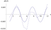 |
Fig. 3. Relative density variations dN/N (dashed line) depending on n in the 14 February 1999 zebra at 12:08:57.0 UT together with the cosine approximation (solid line). |
2.3. 21 April 2002 zebra (Fu et al. 2004; Kuznetsov 2007)
Relative density variations dN/N in dependence on n for this zebra event at 01:45:49.5 UT together with the cosine approximation are shown in Fig. 4. The amplitude and wavelength of the cosine function are A = 0.0032 and Lchar = 5.60, respectively.
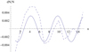 |
Fig. 4. Relative density variations dN/N (dashed line) depending on n in the 21 April 2002 zebra at 01:45:49.5 UT together with the cosine approximation (solid line). |
2.4. 25 October 1994 zebra (Aurass et al. 2003; Zlotnik et al. 2003)
Relative density variations dN/N in dependence on n for this zebra event at 10:08:23.1 UT together with the cosine approximation are shown in Fig. 5. The amplitude and wavelength of the cosine function are A = 0.00098 and Lchar = 2.87, respectively.
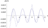 |
Fig. 5. Relative density variations dN/N (dashed line) depending on n in the 25 October 1994 zebra at 10:08:23.1 UT together with the cosine approximation (solid line). |
2.5. 24 February 2011 zebra (Chernov et al. 2015)
Relative density variations dN/N in dependence on n for this zebra event at 07:41:08.8 UT together with the cosine approximation are shown in Fig. 6. The amplitude and wavelength of the cosine function are A = 0.0039 and Lchar = 4.21, respectively.
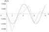 |
Fig. 6. Relative density variations dN/N (dashed line) depending on n in the 24 February 2011 zebra at 07:41:08.8 UT together with the cosine approximation (solid line). |
2.6. 17 August 1998 (Zlotnik et al. 2009)
Relative density variations dN/N in dependence on n for this zebra event at 07:06:31.0 UT together with the cosine approximation are shown in Fig. 7. The amplitude and wavelength of the cosine function are A = 0.0011 and Lchar = 2.09, respectively.
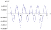 |
Fig. 7. Relative density variations dN/N (dashed line) depending on n in the 17 August 1998 zebra at 07:06:31.0 UT together with the cosine approximation (solid line). |
2.7. The 1 August 2010 (Chernov et al. 2018)
Relative density variations dN/N in dependence on n for this zebra event at 08:21:16.0 UT together with the cosine approximation are shown in Fig. 8. The amplitude and wavelength of the cosine function are A = 0.0044 and Lchar = 6.48, respectively.
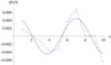 |
Fig. 8. Relative density variations dN/N (dashed line) depending on n in the 1 August 2010 zebra at 08:21:16.0 UT with the cosine approximation (solid line). |
3. Discussion and conclusions
In all analyzed zebras, we found for the zebra-stripe with the lowest frequency f(s1) the gyroharmonic number s1. This enables us to calculate the magnetic field strength and plasma density in the source of this zebra stripe using Eq. (5). The results of the analysis of all studied zebras are summarized in Table 1. Here we present the zebra-stripe frequency f(s1) corresponding to the gyroharmonic number s1, the amplitude A of the cosine approximation of quasi-periodic variations of dN/N, and the corresponding wavelength Lchar, magnetic field strength B, plasma density N, and correlation coefficient C of variations dN/N with the cosine function. In six out of seven analyzed zebras, a rather high correlation coefficient (about 0.7 and higher) between spatial variations of the density and magnetic field and a strictly periodic function was found.
Parameters calculated in the analysis of the zebras.
It follows from this table that for the metric range (frequencies lower than 300 MHz), the average amplitude is 0.00091 ± 0.00023, and for the decimetric range (at frequencies above 1000 MHz), the average amplitude is significantly greater and equals 0.0042 ± 0.0009. On the other hand, the average wavelength Lchar in the metric range is 2.82, and in the decimetric range, it is 5.22. Figure 9 shows the dependence of the amplitude of density variations A on the zebra-stripe frequency f(s1).
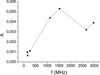 |
Fig. 9. Amplitude of the density variations A in dependence on the zebra-stripe frequency f(s1). |
Table 1 also shows values of the magnetic field strength that are lower than those presented by Tan et al. (2012), for example. However, we analyzed different zebras, and we used a different method. Our method is numerical, and it is based on very general assumptions. The method even includes the varying scales of the plasma density and magnetic field in the region of zebra stripes. Just these varying scales enabled us to find the spatial quasi-periodic variations of the plasma density and magnetic field in zebra sources. The estimated precision in determining the magnetic field strength is 50%.
We express the wavelength Lchar of the density and magnetic field variations in real units. For this purpose, we used the density model of the solar atmosphere by Aschwanden (2002). We took this model because it covers the plasma frequencies of all analyzed zebras and is based on radio observations. We also used the fact that for high values of the gyroharmonic number, the upper hybrid frequency is about equal to the plasma frequency. First, using this density model, we determined the heights of the zebra-stripe sources in the solar atmosphere for the lowest and highest zebra-stripe frequency. Knowing the number of zebra stripes, we calculated the mean distance between the neighboring zebra-stripe sources. By multiplying the wavelength Lchar by this mean distance, we obtained the wavelength L expressed in real units, as shown in Table 2. In Fig. 10 the dependence of L on the zebra frequency is presented.
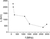 |
Fig. 10. Wavelength L in dependence on the zebra-stripe frequency f(s1). |
Further parameters calculated in the analysis of zebras.
It is known that waves change the magnetic field and density in the plasma and thus can modify them in the regions in which zebra stripes are generated, regardless of whether these waves are standing or propagating. Alfvén waves only change the strength of the magnetic field in their transverse direction and do not change the density of the medium, but they can lead to a displacement of zebra-stripe sources and therefore change the density in these sources.
Furthermore, strong currents can cause filamentation of the magnetic tube structure (Nakariakov et al. 2000), which can also lead to a noticeable deviation of frequencies of zebra stripes as compared with a relatively homogeneous structure. Moreover, Nakariakov et al. (2000) showed that the occurrence of a single slow magnetoacoustic wave can modulate the environment and even generate zebra effects. It is also possible, however, that such a wave can lead to displacements of the regions in which zebra stripes are generated and lead to what we see in our analysis.
Considering these processes, we assumed that the found spatial quasi-periodic variations of the density and magnetic field are caused by the magnetoacoustic waves that stand or propagate in the flux tube in which the zebra-stripe sources are generated. Thus, we can connect the found wavelength L with the period of these waves in the tube.
For the torsional and sausage modes, these periods Pt and Psa are linked with the wavelength of variations L as (Nakariakov & Melnikov 2009)
 (7)
(7)
where for the torsional mode the phase speed Cph is equal to the Alfvén speed  inside the tube, and for the sausage mode
  , where ρe = 0.1 ρ (ρ and ρe is the density in and out of the tube) (Nakariakov et al. 1999). The results for these two modes are shown in Table 2, where R(s1) is the ratio R for the zebra stripe with s = s1, Lchar is the wavelength, L is the wavelength in real units, Pt is the period of wave oscillations of the torsional mode, and Psa is the period of the sausage mode.
Oscillations with the periods shown in Table 2 can exist in coronal loops. For example, oscillations with the periods of several dozen seconds have been observed in the radio, extreme-UV, and X-ray emissions (Huang et al. 2014; Karlický et al. 2020). For shorter periods, see Karlický et al. (2005) and Nakariakov et al. (2016), for instance.
In summary, we discovered spatial quasi-periodic variations of the plasma density and magnetic field in the zebra source. In six out of seven analyzed zebras, a high correlation coefficient of the spatial variations of the density and magnetic field with a strictly periodic function was found. These density and magnetic field variations were explained with magnetoacoustic waves in the loops in which the zebra-stripe sources are located. Wavelengths and periods of these waves were estimated.
Acknowledgments
The authors thank the referee for comments that improved the paper. M. Karlický acknowledges support from the project RVO-67985815 and GA ČR grants 19-09489S, 20-09922J, and 20-07908S. L. V. Yasnov acknowledges support from the Russian Foundation for Basic Research, Grants 18-29-21016-mk, from Program RAN No. 28, Project 1D and State Task No. AAAA-A17-117011810013-4.
References
- Allen, C. W. 1947, MNRAS, 107, 426 [NASA ADS] [Google Scholar]
- Aschwanden, M. J. 2002, Space Sci. Rev., 101, 1 [Google Scholar]
- Aurass, H., Klein, K. L., Zlotnik, E. Y., & Zaitsev, V. V. 2003, A&A, 410, 1001 [NASA ADS] [CrossRef] [EDP Sciences] [Google Scholar]
- Bárta, M., & Karlický, M. 2006, A&A, 450, 359 [NASA ADS] [CrossRef] [EDP Sciences] [Google Scholar]
- Chernov, G. P. 1976, Sov. Astron., 20, 449 [Google Scholar]
- Chernov, G. P. 1990, Sol. Phys., 130, 75 [Google Scholar]
- Chernov, G. P. 2006, Space Sci. Rev., 127, 195 [Google Scholar]
- Chernov, G. 2011, Fine Structure of Solar Radio Bursts, Astrophysics and Space Science Library (Heidelberg: Springer) [Google Scholar]
- Chernov, G., Fomichev, V., Tan, B., et al. 2015, Sol. Phys., 290, 95 [Google Scholar]
- Chernov, G. P., Fomichev, V. V., & Sych, R. A. 2018, Geomag. Aeron., 58, 394 [Google Scholar]
- Dulk, G. A., & McLean, D. J. 1978, Sol. Phys., 57, 279 [NASA ADS] [CrossRef] [Google Scholar]
- Fu, Q., Ji, H., Qin, Z., et al. 2004, Sol. Phys., 222, 167 [Google Scholar]
- Huang, J., Tan, B., Zhang, Y., Karlický, M., & Mészárosová, H. 2014, ApJ, 791, 44 [Google Scholar]
- Kaneda, K., Misawa, H., Iwai, K., et al. 2018, ApJ, 855, L29 [Google Scholar]
- Karlický, M. 2014, A&A, 561, A34 [NASA ADS] [CrossRef] [EDP Sciences] [Google Scholar]
- Karlický, M., & Yasnov, L. 2015, A&A, 581, A115 [NASA ADS] [CrossRef] [EDP Sciences] [Google Scholar]
- Karlický, M., & Yasnov, L. 2018, A&A, 618, A60 [NASA ADS] [CrossRef] [EDP Sciences] [Google Scholar]
- Karlický, M., & Yasnov, L. 2019, A&A, 624, A119 [NASA ADS] [CrossRef] [EDP Sciences] [Google Scholar]
- Karlický, M., & Yasnov, L. 2020, A&A, 638, A22 [EDP Sciences] [Google Scholar]
- Karlický, M., Yan, Y., Fu, Q., et al. 2001, A&A, 369, 1104 [NASA ADS] [CrossRef] [EDP Sciences] [Google Scholar]
- Karlický, M., Bárta, M., Mészárosová, H., & Zlobec, P. 2005, A&A, 432, 705 [NASA ADS] [CrossRef] [EDP Sciences] [Google Scholar]
- Karlický, M., Kašparová, J., & Sych, R. 2020, ApJ, 888, 18 [Google Scholar]
- Kuijpers, J. M. E. 1975, PhD Thesis, Utrecht, Rijksuniversiteit, Doctor in de Wiskunde en Natuurwetenschappen Dissertation [Google Scholar]
- Kuijpers, J. 1980, in Radio Physics of the Sun, eds. M. R. Kundu, & T. E. Gergely, IAU Symp., 86, 341 [Google Scholar]
- Kuznetsov, A. A. 2007, Astron. Lett., 33, 319 [Google Scholar]
- Kuznetsov, A. A., & Tsap, Y. T. 2007, Sol. Phys., 241, 127 [Google Scholar]
- LaBelle, J., Treumann, R. A., Yoon, P. H., & Karlický, M. 2003, ApJ, 593, 1195 [Google Scholar]
- Laptukhov, A. I., & Chernov, G. P. 2009, Plasma Phys. Rep., 35, 160 [Google Scholar]
- Ledenev, V. G., Yan, Y., & Fu, Q. 2006, Sol. Phys., 233, 129 [Google Scholar]
- Mollwo, L. 1983, Sol. Phys., 83, 305 [Google Scholar]
- Mollwo, L. 1988, Sol. Phys., 116, 323 [NASA ADS] [Google Scholar]
- Nakariakov, V. M., & Melnikov, V. F. 2009, Space Sci. Rev., 149, 119 [Google Scholar]
- Nakariakov, V. M., Ofman, L., Deluca, E. E., Roberts, B., & Davila, J. M. 1999, Science, 285, 862 [Google Scholar]
- Nakariakov, V. M., Mendoza-Briceño, C. A., & Ibáñez, S. 2000, ApJ, 528, 767 [Google Scholar]
- Nakariakov, V. M., Pilipenko, V., Heilig, B., et al. 2016, Space Sci. Rev., 200, 75 [Google Scholar]
- Slottje, C. 1981, Atlas of Fine Structures of Dynamics Spectra of Solar Type IV-dm and Some Type II Radio Bursts. Dwingeloo Observatory, The Netherlands [Google Scholar]
- Tan, B., Zhang, Y., Tan, C., & Liu, Y. 2010, ApJ, 723, 25 [Google Scholar]
- Tan, B., Yan, Y., Tan, C., Sych, R., & Gao, G. 2012, ApJ, 744, 166 [Google Scholar]
- Tan, B., Tan, C., Zhang, Y., Mészárosová, H., & Karlický, M. 2014, ApJ, 780, 129 [Google Scholar]
- Winglee, R. M., & Dulk, G. A. 1986, ApJ, 307, 808 [Google Scholar]
- Yasnov, L. V., & Karlický, M. 2020, Sol. Phys., 295, 96 [Google Scholar]
- Zheleznyakov, V. V., & Zlotnik, E. Y. 1975, Sol. Phys., 44, 461 [Google Scholar]
- Zlotnik, E. Y., Zaitsev, V. V., Aurass, H., Mann, G., & Hofmann, A. 2003, A&A, 410, 1011 [NASA ADS] [CrossRef] [EDP Sciences] [Google Scholar]
- Zlotnik, E. Y., Zaitsev, V. V., Aurass, H., & Mann, G. 2009, Sol. Phys., 255, 273 [Google Scholar]
All Tables
All Figures
|
Fig. 1. Difference between the zebra-stripe frequencies fob observed at 03:22:27.4 UT and those fth calculated according to Eq. (3) in dependence on the zebra-stripe frequency. At the lowest frequency, the error bar is shown, calculated from the accuracy in determining the observed zebra-stripe frequencies. |
| In the text | |
|
Fig. 2. Variations computed for the 21 June 2011 zebra at 03:22:27.4 UT. Left: relative variations in magnetic field dB/B (solid line) and plasma density dN/N (dashed line) depending on n. Right: relative plasma density variations (dashed line) depending on n in comparison with a cosine function (solid line) with amplitude A = 0.00064 and wavelength Lchar = 3.50. |
| In the text | |
|
Fig. 3. Relative density variations dN/N (dashed line) depending on n in the 14 February 1999 zebra at 12:08:57.0 UT together with the cosine approximation (solid line). |
| In the text | |
|
Fig. 4. Relative density variations dN/N (dashed line) depending on n in the 21 April 2002 zebra at 01:45:49.5 UT together with the cosine approximation (solid line). |
| In the text | |
|
Fig. 5. Relative density variations dN/N (dashed line) depending on n in the 25 October 1994 zebra at 10:08:23.1 UT together with the cosine approximation (solid line). |
| In the text | |
|
Fig. 6. Relative density variations dN/N (dashed line) depending on n in the 24 February 2011 zebra at 07:41:08.8 UT together with the cosine approximation (solid line). |
| In the text | |
|
Fig. 7. Relative density variations dN/N (dashed line) depending on n in the 17 August 1998 zebra at 07:06:31.0 UT together with the cosine approximation (solid line). |
| In the text | |
|
Fig. 8. Relative density variations dN/N (dashed line) depending on n in the 1 August 2010 zebra at 08:21:16.0 UT with the cosine approximation (solid line). |
| In the text | |
|
Fig. 9. Amplitude of the density variations A in dependence on the zebra-stripe frequency f(s1). |
| In the text | |
|
Fig. 10. Wavelength L in dependence on the zebra-stripe frequency f(s1). |
| In the text | |
Current usage metrics show cumulative count of Article Views (full-text article views including HTML views, PDF and ePub downloads, according to the available data) and Abstracts Views on Vision4Press platform.
Data correspond to usage on the plateform after 2015. The current usage metrics is available 48-96 hours after online publication and is updated daily on week days.
Initial download of the metrics may take a while.