| Issue |
A&A
Volume 646, February 2021
|
|
|---|---|---|
| Article Number | A95 | |
| Number of page(s) | 9 | |
| Section | Extragalactic astronomy | |
| DOI | https://doi.org/10.1051/0004-6361/201937160 | |
| Published online | 16 February 2021 | |
X-ray study of Abell 3365 with XMM-Newton
1
SRON Netherlands Institute for Space Research, Sorbonnelaan 2, 3584 CA Utrecht, The Netherlands
e-mail: This email address is being protected from spambots. You need JavaScript enabled to view it.
2
Leiden Observatory, Leiden University, PO Box 9513, 2300 RA Leiden, The Netherlands
3
Kavli Institute for the Physics and Mathematics of the Universe (WPI), University of Tokyo, Kashiwa 277-8583, Japan
4
Harvard-Smithsonian Center for Astrophysics, 60 Garden Street, Cambridge, MA 0218, USA
5
MTA-Eötvös University Lendület Hot Universe Research Group, Pázmány Péter sétány 1/A, Budapest 1117, Hungary
6
Institute of Physics, Eötvös University, Pázmány Péter sétány 1/A, Budapest 1117, Hungary
7
Istituto di Radio Astronomia, INAF, Via Gobetti 101, 40121 Bologna, Italy
Received:
21
November
2019
Accepted:
4
August
2020
Abstract
We present an X-ray spectral analysis using XMM-Newton/EPIC observations (∼100 ks) of the merging galaxy cluster Abell 3365 (z = 0.093). Previous radio observations suggested the presence of a peripheral elongated radio relic to the east and a smaller radio relic candidate to the west of the cluster center. We find evidence of temperature discontinuities at the location of both radio relics, indicating the presence of a shock with a Mach number of ℳ = 3.5 ± 0.6 towards the east and a second shock with ℳ = 3.9 ± 0.8 towards the west. We also identify a cold front at r ∼ 1.6′ from the X-ray emission peak. Based on the shock velocities, we estimate that the dynamical age of the main merger along the east-west direction is ∼0.6 Gyr. We find that the diffusive shock acceleration scenario from the thermal pool is consistent with the electron acceleration mechanism for both radio relics. In addition, we studied the distribution of the temperature, iron (Fe) abundance, and pseudo-entropy along the merging axis. Our results show that remnants of a metal-rich cool-core can partially or entirely survive after the merging activity. Finally, we find that the merger can displace the metal-rich and low entropy gas from the potential well towards the cold front, as has been suggested via numerical simulations.
Key words: X-rays: galaxies: clusters / galaxies: clusters: intracluster medium
© ESO 2021
1. Introduction
Galaxy clusters are the largest bound structures in the Universe, growing hierarchically through the accretion and merging of less massive subclusters. During this merging process, turbulence, shocks, and cold fronts (CF) arise in the hot intra-cluster medium (ICM) as a result of the strong merging activity (Markevitch & Vikhlinin 2007). Cold fronts delimit the boundary between the infalling subcluster’s cool dense gas and the hot cluster atmosphere. Merger shocks are large-scale structures that propagate along the hot ICM out to the cluster outskirts, where they are usually found. Both can be detected by temperature and density discontinuities in the ICM via spectral analysis and X-ray surface brightness (SB) edges, respectively. Moreover, shocks present a discontinuity also in the pressure distribution, while cold fronts maintain it uniformly across the edge (Vikhlinin et al. 2001). Shocks in galaxy clusters (typically characterized by a Mach number, ℳ ≤ 3–5) are thought to (re)accelerate electrons in the ICM via first-order Fermi diffusive shock acceleration (hereafter DSA, Bell 1987; Blandford & Eichler 1987). These relativistic particles may produce non-thermal synchrotron emission in the form of radio relics in the presence of an amplified magnetic field. These radio features are elongated, polarized, and steep-spectrum (α < −1, being Sν ∝ να) structures that are typically located at the cluster periphery (for a theoretical and observational review, respectively, see Brunetti & Jones 2014; van Weeren et al. 2019). Turbulence generated in the merger may also (re)accelerate particles, generating unpolarized cluster-wide radio phenomena known as radio halos (Brunetti et al. 2001; Feretti et al. 2012; van Weeren et al. 2019).
Today, the number of shock detections in merging galaxy clusters is increasing (see, e.g., Akamatsu et al. 2017; Thölken et al. 2018; Urdampilleta et al. 2018; Di Gennaro et al. 2019; Botteon et al. 2019). In some cases, these shocks appear at the same or a similar location as radio relics (see Table 1 of van Weeren et al. 2019). The study of the shock-relic connection and the relative radial distribution throughout the ICM serves to improve our understanding of the dynamical stage of the cluster, as well as the physics of cosmic ray acceleration. Moreover, a detailed spectral analysis along the merging axis, including a study of their metallicity distribution, can provide valuable information on the chemical evolution and dynamical history of the merged ICM (Urdampilleta et al. 2019).
In this paper, we analyze the temperature and surface brightness discontinuities in the outskirts and central ICM of Abell 3365 (Abell et al. 1989, hereafter A3365), together with the temperature, Fe abundance, and pseudo-entropy distribution along the main merging axis. To this aim, we use observations taken by the XMM-Newton satellite. A3365 is a nearby (z = 0.093, Struble & Rood 1999) multi-merging galaxy cluster detected in X-rays by ROSAT and named RXC J0548.8-2154 (Böhringer et al. 2007). A3365 has M500 = 1.7 × 10¹⁴ M⊙ obtained from X-ray observations (Lovisari & Reiprich 2019). Based on this value and using the self-similar quantities described in Appendix A of Arnaud et al. (2010), we estimate r500 = 0.81 Mpc = 7.82′ (at this redshift) and T500 = 3.14 keV. A3365 hosts one radio relic at the east (hereafter relic E) and one radio relic candidate at the west (hereafter, relic CW) discovered in the NVSS survey and observed by van Weeren et al. (2011) with the VLA and WSRT at 1.4 GHz. As described by van Weeren et al. (2011) relic E and relic CW have an angular extension of 5.5′ or 560 kpc and 2.3′ or 235 kpc, respectively, at this redshift (see Fig. 1).
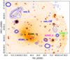 |
Fig. 1. XMM-Newton smoothed image of A3365 in the 0.5–2 keV band. Red circles are the point sources that have been removed. VLA 1.4 GHz radio contours are shown in blue. The center of the three subclusters: A3365_1a, A3365_2 and A3365_3, identified by Golovich et al. (2019) are marked with black, magenta and green crosses, respectively. The X-ray emission peak is shown with a blue cross, A3365_1b. |
A3365 consists of three subclusters (Golovich et al. 2019), see Fig. 1. They all have similar redshifts and the main components, 1 and 3, are separated by a distance of 9′. They are considered part of the same merging system (Golovich et al. 2019), referred to in this paper as A3365. The mass ratio between these two main subclusters is 5:1, (Bonafede et al. 2017). The most massive component 1 has itself two sub-components. The X-ray emission peak (hereafter 1b) is displaced by 2.5′ towards the west from sub-component 1a. The recent spectroscopic survey by Golovich et al. (2019) shows that A3365_3 contains 150 cluster members, is located at a redshift of 0.09273 ± 0.00028 and has a velocity dispersion of 981 ± 58 km s−1. The red sequence distribution suggests that the merging system is formed by three subclusters (see their Fig. 25 for more details): one is coincident with A3365_1a towards the east and the other is in a similar position to A3365_3, namely, in the middle, and the last one is towards the west (hereafter, A3365_2). For more details, see Fig. 1. Golovich et al. (2019), which suggests that the main merging activity occurred along the east-west direction, where A3365 crosses the A3365_1a subcluster, stripping the gas of both subclusters in the east-west direction, intensely disturbing the ICM and forming the cometary tail towards the east. The spatial distribution appears to suggest that the merger between A3365_1a and A3365_3 is associated with the relic E. However, there is no clear connection between this merger and the relic CW, suggesting that it might have a different origin. Golovich et al. (2019) also explain that A3365_1a shows two bright galaxies, which may indicate an ongoing merging activity. Finally, A3365_2 seems to be advancing towards A3365_3, which might be an indication that it has still not merged. Here, we use XMM-Newton to investigate the merging scenario in more detail.
For this analysis, we use the values of protosolar abundances (Z⊙) reported by Lodders et al. (2009). We assume the cosmological parameters H0 = 70 km s−1 Mpc−1, ΩM = 0.27 and ΩΛ = 0.73, respectively, which give 104 kpc per 1 arcmin at z = 0.093. All errors are given at 1σ (68 %) confidence level unless otherwise stated and all the spectral analysis make use of the modified Cash statistics (Cash 1979; Kaastra 2017).
2. Observations and data reduction
The two available XMM-Newton observations of A3365 are listed in Table 1. Both data sets are reduced using the XMM-Newton Science Analysis System (SAS) v17.0.0, with the calibration files from June 2018. For this analysis we use only the observations of the EPIC instrument, containing the MOS and pn detectors. We first apply the standard pipeline commands emproc and epproc. Next, we filter the soft-proton (SP) flares by building Good Time Interval (GTI) files. For this process we use the method detailed in Urdampilleta et al. (2019) and extensively explained in Appendix A.1 of Mernier et al. (2015). We identify and exclude the point sources in the complete FOV with a circular region of 10″ radius (see Fig. 1), except where higher radii are needed to cover larger sources (see Appendix A.2 of Mernier et al. 2015). We use the SAS task edetect_chain for this purpose. We keep the single, double, triple, and quadruple events in MOS (pattern≤12) and only the single pixel events in pn (pattern==0). We also correct the out-of-time events from the pn detector.
Observations and net exposure times.
3. Spectral analysis
In our spectral analysis of A3365, we assume that the observed spectra include the following components: optically thin thermal plasma emission from the ICM in collisional ionization equilibrium and the background consisting of the local hot bubble (LHB), the Milky Way halo (MWH), the cosmic X-ray background (CXB), the hard particle (HP) background, and residual soft-protons (SP). The models used for each of the background components are detailed in Urdampilleta et al. (2019) and Mernier et al. (2015). The estimation of the sky background components (LHB, MHW, and CXB) is obtained from a ROSAT observation of an offset annullus surrounding A3365, using the X-ray Background Tool1. The parameters of the SP components are obtained fitting the total FOV (r = 15′) EPIC spectra, where the ICM cie (SPEX) model parameters are also left free. The best-fit parameters of the background components for each observation are listed in Table 2. The emission models are corrected for the cosmological redshift and absorbed by the galactic interstellar medium. We adopt the weighted total hydrogen column density NH, tot = 2.94 × 1020 cm−2 (Willingale et al. 2013)2.
Best-fit parameter values of the total background estimated for the A3365-p1 and A3365-p2 observations.
The spectral analysis software used in this work is SPEX3 (Kaastra et al. 1996, 2017) version 3.05.00 with SPEXACT (SPEX Atomic Code and Tables) version 3.05.00. We fit simultaneously the spectra of the MOS (energy range from 0.5 to 10 keV) and pn (0.6–10 keV) detectors. We apply the method of optimal binning (Kaastra & Bleeker 2016). A single temperature plasma is assumed for all the sectors in this study. We leave as free parameters the temperature, kT, the metal abundance, Z, and the normalization, Norm. All metal abundances are tied to the Fe abundance. We account for the effect of systematic uncertainties related to the ±10% variation in the normalization of the sky background and non X-ray background components (Mernier et al. 2015; Urdampilleta et al. 2019). The contribution of these systematic uncertainties is further included in our analysis and results.
4. X-ray surface brightness profile
In order to confirm the evidence of shocks and cold fronts characteristic of merging galaxy clusters, the presence of SB profile discontinuities should be found at the same location as temperature discontinuities. We adopt a broken power-law density profile to describe the density. Assuming spherical symmetry, the density distribution is given by:
 (1)
(1)
where n0 is the model density normalization, r is the radius from the center of the sector, rsh is the discontinuity location, and α1 and α2 are the power-law indices. At the location of the SB discontinuity the downstream (post-shock or post-CF) density, n2, is higher by a factor of C = n2/n1 compared with n1, the upstream (pre-shock or pre-CF) density. This factor, C, is known as the compression factor. We assume that the X-ray emissivity is proportional to the density squared (SX ∝ n2) and integrate the cluster emission along the line of sight in the 0.5–2 keV energy band. We subtract the soft proton and the instrumental contribution, and all the point sources are removed. Afterwards, for the sky background, we fit the X-ray SB distribution with a constant model at large radii and we subtract it. Finally, we fit the X-ray SB, leaving all model parameters listed above as free to vary.
5. Results
5.1. Thermodynamical properties at the location of the radio relics
The diffuse radio emission in the A3365 outskirts (see Fig. 1) was classified as a radio relic in the east and a candidate radio relic in the west by van Weeren et al. (2011), as described in Sect. 1. In this work, we investigate the possible presence of shocks associated with these radio relics by analyzing the thermodynamical properties of the hot ICM. We first obtain a temperature radial distribution along both radio relics as shown in Fig. 2. The best-fit parameters are listed in Table 3. We compared their radial temperature profile with the “universal” distribution of Burns et al. (2010) for relaxed clusters. For that purpose, we assume the location of A3365_1a as the centroid, the average temperature as T500 = 3.14 keV, and r200 ∼ 0.65r500 = 12′ (Reiprich et al. 2013). In Fig. 3, both distributions present a clear deviation from the “universal” distribution at the location of the radio relics, which is probably caused by the presence of a shock.
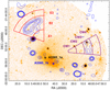 |
Fig. 2. Same as Fig. 1 and indicating spectral extraction regions. The red and purple sectors represent the temperature radial distribution across relic E and CW, respectively. The center of A3365_1a and A3365_1b are marked with black and blue crosses. |
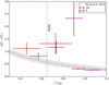 |
Fig. 3. Temperature distribution of the red and purple sectors of Fig. 2 compared with the Burns et al. (2010) “universal” profile for relaxed clusters. The gray shaded area shows the 1σ scatter. |
Furthermore, we can calculate the average electron density as ne ∼ 1.2nH in the sectors shown in Fig. 2, given that Norm = nenHV. The Norm values are taken from the best-fit parameters listed in Table 3. V is the emitting volume projected along the line-of-sight (LOS). We assume that only the sphere between the maximum and minimum radius corresponding to each circular sector contributes to the emission (Henry et al. 2004; Mahdavi et al. 2005). We estimate V as V = 2SL/3, with  , and S is the area of the sectors in the plane of the sky. The density radial distributions along both radio relics are plotted in Fig. 4. The distribution to the west shows a clear density discontinuity at the candidate radio relic edge, consistent with the temperature discontinuity, while a smoother gradient is present at the east.
Next we analyze more specific regions centered on the post and pre-shocks of each radio relic. In order to search for a possible temperature discontinuity, we performed a spectral analysis of the post-shock and pre-shock E and CW regions (see Fig. 5), assuming that the candidate shocks are located at the external edge of the respective radio relics. We maintain a separation between upstream and downstream regions of ≈1′ to avoid any photon leakage from the brighter region. The Fe abundance is fixed to 0.3 Z⊙ in these regions. The best-fit parameters for the post and pre-shock regions at the relics E and CW are shown in Table 4. They both show a significant drop of the temperature. Shocks are characterized by higher temperature and pressure in the post-shock (downstream) than in the pre-shock (upstream) region. The temperature jumps (kTpost/kTpre) are 4.6 ± 1.4 and 5.5 ± 1.2 for E and CW, respectively.
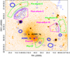 |
Fig. 5. Same as Fig. 1 and indicating spectral extraction regions. The green sectors represent the pre-shock and pre-cold front regions of relic E, relic CW, and CF. The magenta sectors are the post-shock and post-cold front regions. The center of A3365_1a and A3365_1b are marked with black and blue crosses. |
We also analyzed three regions (see red circular sectors in Fig. 6 left) orthogonal to the merging axis. We have compared their radial temperature profile with the “universal” distribution of Burns et al. (2010) for relaxed clusters. As shown in Fig. 6 (right), the temperature profile in this direction presents a smooth decrease and is consistent with the expected distribution for relaxed clusters.
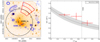 |
Fig. 6. Left panel: same as Fig. 1, showing extraction regions for the “relaxed” direction of the cluster (orthogonal to the merging axis) in red. The black dashed circle represents r500. The center of A3365_1a and A3365_1b are marked with black and blue crosses. Right panel: temperature distribution of the red sectors compared with the Burns et al. (2010) “universal” profile for relaxed clusters. The gray shaded area shows the 1σ scatter. |
In these faint peripheral regions, the surface brightness profiles for the sectors corresponding to the E and W temperature jumps would need to be very heavily binned in order to detect a cluster signal. Therefore, we do not have sufficient measurements to fit a broken-power law model to these profiles that would allow us to constrain the underlying density jump. Nevertheless, we can estimate the density in the coarse regions used to determine the temperature jumps. These the density jumps should be considered as the upper limits.
For the relic E, we estimate n1 = (0.52 ± 0.11) × 10−4 cm−3 and n2 = (1.64 ± 0.04) × 10−4 cm−3. The compression factor derived from these densities is C = 3.2 ± 0.7, which is in very good agreement with the value obtained from the temperature jump listed in Table 7. For the relic CW, the density values are n1 = (0.97 ± 0.10) × 10−4 cm−3 and n2 = (2.41 ± 0.06) × 10−4 cm−3. In this case, the compression factor is C = 2.5 ± 0.3. This value is lower but close to the C derived from the temperature discontinuity described in Table 7. For the E and CW relics, therefore, both the density and temperature profiles exhibit evidence that would support the presence of a shock.
5.2. Substructure in the central ICM
We searched for the X-ray SB discontinuity in different edges of the bright and disturbed ICM. We find a clear discontinuity in the western side, close to the X-ray peak. For the X-ray SB profile analysis, we use a circular sector centered on the X-ray peak, with exactly the same shape as the post-CF (magenta) and pre-CF (green) regions together; see Fig. 5. The radial X-ray SB profile obtained is shown in Fig. 7. The best-fit parameters of the model show a discontinuity at rsh = 1.57 ± 0.05 arcmin with a compression factor value of C = 1.33 ± 0.08. At this same location, we measure the temperature in the post-CF (r = 0′–1.57′) and pre-CF (r = 1.57′–3.5′) regions (see Fig. 5 and Table 5) and we obtain a temperature jump of T1/T2 = 0.79 ± 0.05. Using the temperature jump and the compression factor, we obtain a pressure ratio of P1/P2 = 1.05 ± 0.09, consistent with a constant pressure value across the edge. This proves that the X-ray discontinuity found in the disturbed ICM edge is a cold front.
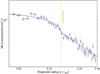 |
Fig. 7. Radial X-ray SB profile across the cold front in the 0.5–2.0 keV band using the XMM-Newton observations. The profile is corrected for exposure, background and soft protons, and point sources are removed. The best-fit model is shown in blue and the vertical dashed orange line represents the estimated position of the cold front. |
5.3. Temperature and Fe abundance distributions along the merging axis
As shown in Fig. 8, we cover the disturbed ICM elongation with circular sectors following the X-ray emission in the east-west direction. We dedicate two circles to the subcore of the main subcluster, A3365_1a, and X-ray peak (A3365_1b). We fit the cluster emission and the background spectra, excluding the point sources as explained in Sect. 3. We use the X-ray emission peak as the centroid for our temperature and abundance distributions along the merging axis (see Fig. 9).
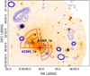 |
Fig. 8. Same as Fig. 1, where the red sectors represent the regions used for the temperature and abundance distributions. The cyan line shows the location of the cold front. The center of A3365_1a and the A3365_1b are marked with black and blue crosses. |
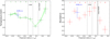 |
Fig. 9. Left panel: temperature distribution of A3365 along the merging direction. Right panel: abundance distribution of A3365. The shaded area in the left panel represent the systematic uncertainties. Systematic errors on abundance are much smaller than statistical and thus not shown in the right panel. |
The best-fit parameters of the temperature and abundance distributions are presented in Table 6. Sectors one to five, which are contained in the cometary tail, have a uniform temperature distribution between 3–3.5 keV. However, the temperature clearly decreases downstream of the cold front, increasing with a significant gradient in the cold front upstream region. The abundance distribution shows some signatures of two enhanced peaks, one associated with the main subcluster core, A3365_1a, and the other one with the cold front downstream region, both with values close to ∼0.6 Z⊙. The gas located just behind the cold front is displaced from the central potential well by the internal dynamical forces of the cold front (Heinz et al. 2003). These same effects have been already observed in Abell 3667 and Abell 665 (Lovisari et al. 2009; Urdampilleta et al. 2019).
6. Discussion
6.1. Shock jump conditions and properties
Based on the temperature jump found in the A3365 merging galaxy cluster outskirts, we report the presence of two X-ray shock candidates associated with the relic E and relic CW. Here, we present the shock properties (the Mach number, ℳ, the compression factor, C, and the shock velocity, vshock, among others); see Table 7. The ℳ and C are calculated from the Rankine-Hugoniot jump condition (Landau & Lifshitz 1959) and assuming that all of the dissipated shock energy is thermalized and the ratio of specific heats (the adiabatic index) is γ = 5/3:
 (2)
(2)
 (3)
(3)
Shock properties at relic E and relic CW.
where n is the density, and the indices 2 and 1 correspond to post-shock and pre-shock regions, respectively.
The Mach numbers estimated from the temperature discontinuities described in the previous section are ℳE = 3.5 ± 0.6 and ℳCW = 3.9 ± 0.8. The presence of shocks with ℳ ≳3.0 is uncommon in galaxy clusters, with only few examples known until now (CIZA J224.8+5301, Akamatsu et al. 2015; “Bullet”, Shimwell et al. 2015; “El Gordo”, Botteon et al. 2016; A665, Dasadia et al. 2016; A3376, Urdampilleta et al. 2018).
The sound speed at the pre-shock regions is cs, E ∼ 508 km s−1 and cs, W ∼ 479 km s−1, assuming cs =  where μ = 0.6. The shock propagation speed vshock = ℳ ⋅ cs for the east and west is vshock, E = 1800 ± 300 km s−1 and vshock, W = 1900 ± 300 km s−1, respectively. If we assume that the eastern shock is generated by the merger of A3365_1a and A3365_3 and it is moving with a constant velocity, we can calculate the dynamical age of the merger. The projected distance between A3365_1a and the relic E is ∼10′, which means ∼1.04 Mpc at z = 0.093. Thus, the time required to reach the actual position is ∼0.6 Gyr. We carry out the same exercise with the shock in the west, assuming that is generated by the same merger. In this case, the distance between A3365_1a and relic CW is ∼11′ = 1.17 Mpc, resulting in a time of ∼0.6 Gyr. The upper limit of the merging time using the downstream gas velocity is, in both cases, ∼2.0 Gyr. Therefore, both shocks required the same time to propagate from the core passage up to their current location. We have no evidence of additional physical processes or mechanisms for the generation of the western shock. This might suggest that the possible origin of both shocks is the merger between A3365_1a and A3365_3.
As we explain in Sect. 1, the DSA is based on first-order Fermi acceleration and considers that there is a stationary and continuous injection. It accelerates relativistic electrons following a power-law spectrum n(E)dE ∼ E−pdE with p = (C + 2)/(C − 1), producing a radio synchrotron emission whose emissivity depends on the frequency as Sv ∝ vα. The two power law indexes p and the radio injection spectral index α are related α = − (p − 1)/2. From our analysis, we estimate the injection spectral index values of αE = −0.68 ± 0.06 and αW = −0.64 ± 0.03. Unfortunately, there are no available spectral indices derived from radio observations for their comparison to date. Future radio observations are needed to confirm these results.
6.2. Shock acceleration efficiency
Recent studies have demonstrated that the low efficiency of the DSA mechanism for low-ℳ shocks (ℳ ≤ 2–2.5) is not enough for the electron acceleration to proceed from the thermal pool (for observational evidence on radio relics, see Botteon et al. 2020 and theoretical arguments, Vink & Yamazaki 2014, Ha et al. 2018 and Ryu et al. 2019). For this reason, alternative mechanisms have been proposed lately, as for example the re-acceleration of pre-existing cosmic ray electrons (Markevitch et al. 2005; Kang et al. 2012; Fujita et al. 2015).
In this case, if we assume DSA as the shock acceleration mechanism of the thermal electrons in radio relics, the electron acceleration efficiency, ηe, can be defined as the amount of kinetic energy flux at the shock moving at vshock, which is converted into relativistic electrons and produces the synchrotron luminosity Lsync of the radio relic. Both parameters, ηe and Lsync, are related according to (Brunetti & Jones 2014):
![Mathematical equation: $$ \begin{aligned} \eta _{\rm {e}}=\Bigg [\frac{1}{2}\rho _1{ v}_{\rm {shock}}^3\Big (1-\frac{1}{C^2}\Big )\frac{B^2}{B^2+B_{\rm {CMB}}^2}S\Bigg ]^{-1}\Psi (\mathcal{M})L_{\rm {sync}}, \end{aligned} $$](/articles/aa/full_html/2021/02/aa37160-19/aa37160-19-eq7.gif) (4)
(4)
where ρ1 is the total upstream density, C the compression factor, S the shock surface, BCMB = 3.25(1+z)2 and B are the magnetic field equivalent for the cosmic microwave background radiation (CMBR) and the magnetic field for the radio relic in μG, respectively. The Ψ(ℳ) represents the ratio between the energy flux injected into “all” particles and those that are only visible in radio (for a more detailed description of the computation and equations, see Botteon et al. 2020).
Figure 10 shows the electron acceleration efficiency, ηe, as a function of the magnetic field, B, at both relics. For the relic E we assume S1.4 GHz = 38.9 mJy and S = π × ((LLS/2)2) = π × ((644/2)2) kpc2 with LLS being the radio relic largest linear size (see Nuza et al. 2017). The temperature and electron density in the downstream region are kTd = 4.45 keV and nd = 1.64 × 10⁻⁴ cm−3, respectively. For the relic CW we assume S1.4 GHz = 5.4 mJy, S = π × ((LLS/2)2) = π × ((235/2)2) kpc2 (see van Weeren et al. 2011), kTd = 4.72 keV and nd = 2.41 × 10⁻⁴ cm−3. The density in the upstream region is obtained from the Eq. (3). The minimum momentum of electrons in both cases has been selected as pmin = 0.1mec. We calculated ηe values for a lower value of pmin = 0.08mec, based on the Figs. 1 and 2 of Botteon et al. (2020), and the difference can be neglected. We obtain ηe values for three different Mach numbers of ℳ = 3.0, 3.5 and 4.0. In the case of ℳ = 3.5, for B > 0.4 μG, the electron acceleration efficiency due to the shock is ηe ≲ 10−3 for both relics. Therefore, in this case the standard DSA scenario cannot be excluded, where efficiencies of this order are expected for weak shocks (Brunetti & Jones 2014; Caprioli & Spitkovsky 2014; Hong et al. 2014; Ha et al. 2018). These results also agree with the recent findings of Botteon et al. (2020) and Botteon et al. (2016) for “El Gordo” cluster, which suggest that DSA of thermal electrons is a valid mechanism in the case of shocks with high Mach number (ℳ ≥ 3).
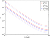 |
Fig. 10. Electron acceleration efficiency, ηe as a function of the magnetic field, B, for ℳ = 3.0, 3.5 and 4.0. Calculations assume a minimum momentum of electrons pmin = 0.1mec. |
6.3. Cold front properties
We find evidence of X-ray SB and temperature discontinuities at the western edge of the highly disturbed ICM associated with a cold front. This front is perpendicular to the merging axis and moves presumably in the east-west direction, as shown in Fig. 5. It confines a cool and dense gas cloud moving through a hotter ambient gas (Markevitch & Vikhlinin 2007; Vikhlinin et al. 2001). The velocity of this cool gas cloud can be estimated using the density and temperature values derived from the X-ray SB and temperature discontinuities (Landau & Lifshitz 1959; Vikhlinin et al. 2001; Ichinohe et al. 2017; Urdampilleta et al. 2018). For that purpose, we assume that the cool gas is a spherical body moving through the ambient gas.
The ratio of pressures between the stagnation point (index 0, where the fluid v = 0, in front of the blob) and the free stream (index 1) can be expressed as a function of the gas cloud speed v (or equivalently the Mach number assuming ℳ1 = v/cs, where cs is sound velocity of the free stream) (Landau & Lifshitz 1959):
 (5)
(5)
where γ = 5/3 is the adiabatic index.
The gas dynamic parameters at the stagnation point cannot be measured directly. However, the pressure in the downstream region of the cold front has a similar value as the stagnation pressure as explained by Vikhlinin et al. (2001). For this reason, we assume T0 = 2.62 ± 0.10 keV as the temperature downstream the cold front and T1 = 3.30 ± 0.17 keV as the free stream region, upstream (Vikhlinin et al. 2001; Sarazin et al. 2016). The density of these regions is calculated from the best-fit parameter of the broken power-law model described in Sect. 4 and shown in Fig. 7. The pressure inside the cold front is p0 = T0 × n0 = 7.7 × 10⁻³ ± 1.0 × 10⁻³ keV cm−3 and outside p1 = T1 × n1 = 4.2 × 10⁻³ ± 0.6 × 10⁻³ keV cm−3 (both densities are calculated at the average point of the downstream and upstream regions). Thus, the pressure ratio is p0/p1 = 1.9 ± 0.4, which corresponds to a subsonic Mach number of ℳ1 = 0.92 ± 0.07 in the free stream. This value is consistent with the cold front in A3376 (ℳ1 = 1.2 ± 0.2, Urdampilleta et al. 2018) and slightly higher than A3667 (ℳ1 = 0.70 ± 0.06, Ichinohe et al. 2017). The sound speed in this region is ccf =  = 937 ± 24 km s−1 with kT1 = 3.30 ± 0.17 keV, giving the velocity of the cool gas cloud as vcf = 862 ± 69 km s−1.
6.4. Pseudo-entropy distribution
We aim to better understand the thermal history of the disturbed ICM of A3365. For that reason, we calculate the pseudo-entropy, K ≡ kT × n−2/3, for each of the sectors described in Sect. 5.3. We use the data obtained from the spectral analysis, namely the temperature, kT, and the emission measure, Norm, to derive the density, n.
Figure 11 shows the pseudo-entropy distribution along the merging axis together with the Fe abundance profile. The distribution shows a clear low entropy minimum at the location of the X-ray peak of the merging system. Urdampilleta et al. (2019) observed the same behavior in two of the merging clusters Abell 665 and 1RXS J0603.3+4214 (known as the Toothbrush cluster). This suggests that the cool-core of the progenitor subcluster has totally or partially remained after the merging activity. As a consequence, we may be in the presence of a cool-core remnant (Rossetti & Molendi 2010). Moreover, the presence of the Fe abundance enhancement and the low temperature gas towards the contact discontinuity or cold front, supports the scenario described by the simulations of Heinz et al. (2003). As an effect of the merger, the cold dense core of the cluster is displaced from the center of the potential well. As the velocity of the core reverses in an attempt to return to equilibrium, a shear layer is created driving the gas along the cold front backwards in the direction of the background flow. This brings the material with the lowest temperature and highest abundance from the center of the cool core towards the cold front, as shown by our results in Fig. 11.
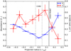 |
Fig. 11. Scaled pseudo-entropy (K/1000) and abundance distributions along the merging axis for A3365. |
7. Summary
In this work, we present an imaging and spectral analysis of A3365 (z = 0.093) using XMM-Newton observations (∼100 ks). The recent spectroscopic survey by Golovich et al. (2019) demonstrates that A3365 is a complex merging system formed by three subclusters. Moreover, previous radio observations (van Weeren et al. 2011) suggest this merging galaxy cluster hosts a radio relic to the east and a radio relic candidate to the west of the merging cluster center.
Here, we detect abrupt temperature jumps across both radio relic edges, suggesting the presence of two shocks associated with them in the cluster outskirts. For these shocks, we estimate the Mach number and the shock velocity based on the temperature jump, namely, ℳ = 3.5 ± 0.6 and vshock ∼ 1800 ± 300 for the shock in the east, and ℳ = 3.9 ± 0.8 and vshock ∼ 1900 ± 300 for the shock in the west. Assuming that they are moving with constant velocity, the time since core passage is ∼0.6 Gyr for both shocks. This might suggest that they originate in the same merger between A3365_1a and A3365_3. We compute the shock acceleration efficiency as a function of the magnetic field in the both relics and we find that DSA scenario is a possible acceleration mechanism. Similar results have been found for shocks with ℳ ≥ 3 as “El Gordo” (Botteon et al. 2016) and A3376 (Botteon et al. 2020).
We also confirm, based on temperature and surface brightness discontinuities, the presence of a cold front at r∼1.6′ from the X-ray emission peak in the merging direction. It delimits a cool gas cloud moving with ℳ ∼ 0.9 and a speed of v ∼ 860 km s−1.
In addition, we obtain the temperature, Fe abundance, and pseudo-entropy distribution in the highly disturbed central parts of the ICM along the merging axis. We find signatures of two abundance peaks, one that is coincident with A3365_1a (∼0.6 Z⊙) and another that is located towards the cold front (∼0.6 Z⊙) and displaced from the potential well. This is consistent with the simulations of Heinz et al. (2003), which suggest that the shock passage can affect the internal dynamics of the cool gas and move the low entropy and metal rich gas towards the cold front. Finally, in line with previous results shown in, for example, Urdampilleta et al. (2019), the pseudo-entropy distribution shows a relative low-entropy minimum, which might suggest that remnants of the metal-rich cool-core can survive partially or fully after the merging activity.
Acknowledgments
The authors thank Dr. R. van Weeren for the VLA radio data. A. Simionescu is supported by the Women In Science Excel (WISE) programme of the Netherlands Organisation for Scientific Research (NWO), and acknowledges the MEXT World Premier Research Center Initiative (WPI) and the Kavli IPMU for the continued hospitality. SRON is supported financially by NWO, the Netherlands Organization for Scientific Research. This work is based on observations obtained with XMM-Newton, an ESA science mission with instruments and contributions directly funded by ESA member states and the USA (NASA).
References
- Abell, G. O., Corwin, H. G., Jr, & Olowin, R. P. 1989, ApJS, 70, 1 [NASA ADS] [CrossRef] [EDP Sciences] [Google Scholar]
- Akamatsu, H., van Weeren, R. J., Ogrean, G. A., et al. 2015, A&A, 582, A20 [Google Scholar]
- Akamatsu, H., Mizuno, M., Ota, N., et al. 2017, A&A, 600, A100 [NASA ADS] [CrossRef] [EDP Sciences] [Google Scholar]
- Arnaud, M., Pratt, G. W., Piffaretti, R., et al. 2010, A&A, 517, A92 [NASA ADS] [CrossRef] [EDP Sciences] [Google Scholar]
- Bell, A. R. 1987, MNRAS, 225, 615 [NASA ADS] [Google Scholar]
- Blandford, R., & Eichler, D. 1987, Phys. Rep., 154, 1 [Google Scholar]
- Böhringer, H., Schuecker, P., Pratt, G. W., et al. 2007, A&A, 469, 363 [NASA ADS] [CrossRef] [EDP Sciences] [Google Scholar]
- Bonafede, A., Cassano, R., Bruggen, M., et al. 2017, MNRAS, 470, 3465 [NASA ADS] [CrossRef] [Google Scholar]
- Botteon, A., Gastaldello, F., Brunetti, G., & Kale, R. 2016, MNRAS, 463, 1534 [NASA ADS] [CrossRef] [Google Scholar]
- Botteon, A., Shimwell, T. W., Bonafede, A., et al. 2019, A&A, 622, A19 [NASA ADS] [CrossRef] [EDP Sciences] [Google Scholar]
- Botteon, A., Brunetti, G., Ryu, D., & Roh, S. 2020, A&A, 634, A64 [NASA ADS] [CrossRef] [EDP Sciences] [Google Scholar]
- Brunetti, G., & Jones, T. W. 2014, IJMPD, 23, 1430007 [Google Scholar]
- Brunetti, G., Setti, G., Feretti, L., & Giovannini, G. 2001, MNRAS, 320, 365 [NASA ADS] [CrossRef] [Google Scholar]
- Burns, J. O., Skillman, S. W., & O’Shea, B. W. 2010, ApJ, 721, 1105 [Google Scholar]
- Caprioli, D., & Spitkovsky, A. 2014, ApJ, 783, 91 [NASA ADS] [CrossRef] [Google Scholar]
- Cash, W. 1979, ApJ, 228, 939 [NASA ADS] [CrossRef] [Google Scholar]
- Dasadia, S., Sun, M., Sarazin, C., et al. 2016, ApJ, 820, L20 [Google Scholar]
- Di Gennaro, G., van Weeren, R. J., Andrade-Santos, F., et al. 2019, ApJ, 873, 64 [NASA ADS] [CrossRef] [Google Scholar]
- Feretti, L., Giovannini, G., Govoni, F., & Murgia, M. 2012, A&ARv, 20, 54 [Google Scholar]
- Fujita, Y., Takizawa, M., Yamazaki, R., Akamatsu, H., & Ohno, H. 2015, ApJ, 815, 116 [NASA ADS] [CrossRef] [Google Scholar]
- Golovich, N., Dawson, W. A., Wittman, D. M., et al. 2019, ApJ, 882, 69 [Google Scholar]
- Ha, J.-H., Ryu, D., & Kang, H. 2018, ApJ, 857, 26 [NASA ADS] [CrossRef] [Google Scholar]
- Heinz, S., Churazov, E., Forman, W., Jones, C., & Briel, U. G. 2003, MNRAS, 346, 13 [Google Scholar]
- Henry, J. P., Finoguenov, A., & Briel, U. G. 2004, ApJ, 615, 181 [NASA ADS] [CrossRef] [Google Scholar]
- Hong, S. E., Ryu, D., Kang, H., & Cen, R. 2014, ApJ, 785, 133 [NASA ADS] [CrossRef] [Google Scholar]
- Ichinohe, Y., Simionescu, A., Werner, N., & Takahashi, T. 2017, MNRAS, 467, 3662 [NASA ADS] [CrossRef] [Google Scholar]
- Kaastra, J. S. 2017, A&A, 605, A51 [NASA ADS] [CrossRef] [EDP Sciences] [Google Scholar]
- Kaastra, J. S., & Bleeker, J. A. M. 2016, A&A, 587, A151 [NASA ADS] [CrossRef] [EDP Sciences] [Google Scholar]
- Kaastra, J. S., Mewe, R., & Nieuwenhuijzen, H. 1996, 11th Colloquium on UV and X-ray Spectroscopy of Astrophysical and Laboratory Plasmas, 411 [Google Scholar]
- Kaastra, J. S., Raassen, A. J. J., de Plaa, J., & Gu, L. 2017, https://doi.org/10.5281/zenodo.2272992 [Google Scholar]
- Kang, H., Ryu, D., & Jones, T. W. 2012, ApJ, 756, 97 [Google Scholar]
- Landau, L. D., & Lifshitz, E. M. 1959, Fluid Mechanics, Course of Theoretical Physics (Oxford: Pergamon Press) [Google Scholar]
- Lodders, K., Palme, H., & Gail, H. P. 2009, Landolt Bömstein, New Series, Astronomy and Astrophysics (Springer Verlag), 560 VI/4B [Google Scholar]
- Lovisari, L., & Reiprich, T. H. 2019, MNRAS, 483, 540 [NASA ADS] [CrossRef] [Google Scholar]
- Lovisari, L., Kapferer, W., Schindler, S., & Ferrari, C. 2009, A&A, 508, 191 [NASA ADS] [CrossRef] [EDP Sciences] [Google Scholar]
- Mahdavi, A., Finoguenov, A., Böhringer, H., Geller, M. J., & Henry, J. P. 2005, ApJ, 622, 187 [Google Scholar]
- Markevitch, M., & Vikhlinin, A. 2007, Phys. Rep., 443, 1 [NASA ADS] [CrossRef] [EDP Sciences] [Google Scholar]
- Markevitch, M., Govoni, F., Brunetti, G., & Jerius, D. 2005, ApJ, 627, 733 [NASA ADS] [CrossRef] [Google Scholar]
- Mernier, F., de Plaa, J., Lovisari, L., et al. 2015, A&A, 575, A37 [Google Scholar]
- Nuza, S. E., Gelszinnis, J., Hoeft, M., & Yepes, G. 2017, MNRAS, 470, 240 [NASA ADS] [CrossRef] [Google Scholar]
- Reiprich, T. H., Basu, K., Ettori, S., et al. 2013, Space Sci. Rev., 177, 195 [NASA ADS] [CrossRef] [EDP Sciences] [Google Scholar]
- Rossetti, M., & Molendi, S. 2010, A&A, 510, A83 [Google Scholar]
- Ryu, D., Kang, H., & Ha, J.-H. 2019, ApJ, 883, 60 [NASA ADS] [CrossRef] [Google Scholar]
- Sarazin, C. L., Finoguenov, A., Wik, D. R., & Clarke, T. E. 2016, ArXiv e-prints [arXiv:1606.07433] [Google Scholar]
- Shimwell, T. W., Markevitch, M., Brown, S., et al. 2015, MNRAS, 449, 1486 [NASA ADS] [CrossRef] [Google Scholar]
- Struble, M. F., & Rood, H. J. 1999, ApJS, 125, 35 [NASA ADS] [CrossRef] [Google Scholar]
- Thölken, S., Reiprich, T. H., Sommer, M. W., & Ota, N. 2018, A&A, 619, A68 [NASA ADS] [CrossRef] [EDP Sciences] [Google Scholar]
- Urdampilleta, I., Akamatsu, H., Mernier, F., et al. 2018, A&A, 618, A74 [NASA ADS] [CrossRef] [EDP Sciences] [Google Scholar]
- Urdampilleta, I., Mernier, F., Kaastra, J. S., et al. 2019, A&A, 629, A31 [CrossRef] [EDP Sciences] [Google Scholar]
- van Weeren, R. J., Brüggen, M., Röttgering, H. J. A., et al. 2011, A&A, 533, A35 [NASA ADS] [CrossRef] [EDP Sciences] [Google Scholar]
- van Weeren, R. J., de Gasperin, F., Akamatsu, H., et al. 2019, Space Sci. Rev., 215, 16 [NASA ADS] [CrossRef] [Google Scholar]
- Vikhlinin, A., Markevitch, M., & Murray, S. S. 2001, ApJ, 551, 160 [NASA ADS] [CrossRef] [Google Scholar]
- Vink, J., & Yamazaki, R. 2014, ApJ, 780, 125 [NASA ADS] [CrossRef] [Google Scholar]
- Willingale, R., Starling, R. L. C., Beardmore, A. P., Tanvir, N. R., & O’Brien, P. T. 2013, MNRAS, 431, 394 [NASA ADS] [CrossRef] [Google Scholar]
All Tables
Best-fit parameter values of the total background estimated for the A3365-p1 and A3365-p2 observations.
All Figures
|
Fig. 1. XMM-Newton smoothed image of A3365 in the 0.5–2 keV band. Red circles are the point sources that have been removed. VLA 1.4 GHz radio contours are shown in blue. The center of the three subclusters: A3365_1a, A3365_2 and A3365_3, identified by Golovich et al. (2019) are marked with black, magenta and green crosses, respectively. The X-ray emission peak is shown with a blue cross, A3365_1b. |
| In the text | |
|
Fig. 2. Same as Fig. 1 and indicating spectral extraction regions. The red and purple sectors represent the temperature radial distribution across relic E and CW, respectively. The center of A3365_1a and A3365_1b are marked with black and blue crosses. |
| In the text | |
|
Fig. 3. Temperature distribution of the red and purple sectors of Fig. 2 compared with the Burns et al. (2010) “universal” profile for relaxed clusters. The gray shaded area shows the 1σ scatter. |
| In the text | |
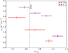 |
Fig. 4. Radial electron density distribution of the red and purple sectors of Fig. 2. |
| In the text | |
|
Fig. 5. Same as Fig. 1 and indicating spectral extraction regions. The green sectors represent the pre-shock and pre-cold front regions of relic E, relic CW, and CF. The magenta sectors are the post-shock and post-cold front regions. The center of A3365_1a and A3365_1b are marked with black and blue crosses. |
| In the text | |
|
Fig. 6. Left panel: same as Fig. 1, showing extraction regions for the “relaxed” direction of the cluster (orthogonal to the merging axis) in red. The black dashed circle represents r500. The center of A3365_1a and A3365_1b are marked with black and blue crosses. Right panel: temperature distribution of the red sectors compared with the Burns et al. (2010) “universal” profile for relaxed clusters. The gray shaded area shows the 1σ scatter. |
| In the text | |
|
Fig. 7. Radial X-ray SB profile across the cold front in the 0.5–2.0 keV band using the XMM-Newton observations. The profile is corrected for exposure, background and soft protons, and point sources are removed. The best-fit model is shown in blue and the vertical dashed orange line represents the estimated position of the cold front. |
| In the text | |
|
Fig. 8. Same as Fig. 1, where the red sectors represent the regions used for the temperature and abundance distributions. The cyan line shows the location of the cold front. The center of A3365_1a and the A3365_1b are marked with black and blue crosses. |
| In the text | |
|
Fig. 9. Left panel: temperature distribution of A3365 along the merging direction. Right panel: abundance distribution of A3365. The shaded area in the left panel represent the systematic uncertainties. Systematic errors on abundance are much smaller than statistical and thus not shown in the right panel. |
| In the text | |
|
Fig. 10. Electron acceleration efficiency, ηe as a function of the magnetic field, B, for ℳ = 3.0, 3.5 and 4.0. Calculations assume a minimum momentum of electrons pmin = 0.1mec. |
| In the text | |
|
Fig. 11. Scaled pseudo-entropy (K/1000) and abundance distributions along the merging axis for A3365. |
| In the text | |
Current usage metrics show cumulative count of Article Views (full-text article views including HTML views, PDF and ePub downloads, according to the available data) and Abstracts Views on Vision4Press platform.
Data correspond to usage on the plateform after 2015. The current usage metrics is available 48-96 hours after online publication and is updated daily on week days.
Initial download of the metrics may take a while.