| Issue |
A&A
Volume 645, January 2021
|
|
|---|---|---|
| Article Number | L6 | |
| Number of page(s) | 5 | |
| Section | Letters to the Editor | |
| DOI | https://doi.org/10.1051/0004-6361/202039902 | |
| Published online | 11 January 2021 | |
Letter to the Editor
Detecting prolonged activity minima in binary stars
The case of ζ2 Reticuli⋆,⋆⋆
1
Instituto de Ciencias Astronómicas, de la Tierra y del Espacio (ICATE), España Sur 1512, CC 49, 5400 San Juan, Argentina
e-mail: This email address is being protected from spambots. You need JavaScript enabled to view it.
2
Instituto de Astronomía y Física del Espacio (IAFE), Buenos Aires, Argentina
3
Facultad de Ciencias Exactas, Físicas y Naturales, Universidad Nacional de San Juan, San Juan, Argentina
4
Departamento de Física, Facultad de Ciencias Exactas y Naturales, Universidad de Buenos Aires, Buenos Aires, Argentina
5
Consejo Nacional de Investigaciones Científicas y Técnicas (CONICET), Argentina
6
Departamento de Física y Astronomía, Universidad de La Serena, Av. Cisternas 1200, La Serena, Chile
7
Universidade de São Paulo, Departamento de Astronomia do IAG/USP, Rua do Matão 1226, Cidade Universitária, 05508-900 São Paulo, SP, Brazil
Received:
13
November
2020
Accepted:
14
December
2020
Abstract
Context. It is well known that from 1645 to 1715 solar activity was notably low and the number of sunspots was extremely reduced. This epoch is known as the Maunder minimum (MM). The study of stars in prolonged activity minima such as the MM could help to shed light on this enigmatic epoch. However, to date, it is not easy to identify MM candidates among other stars. An original idea, which has hardly been explored, is to compare the activity levels of both components of binary systems.
Aims. Our goal is to explore if the star ζ2 Ret, which belongs to a binary system, is in (or going to) a state similar to the MM. We have collected more than 430 spectra acquired between 2000 and 2019 with the HARPS, REOSC, UVES, and FEROS spectrographs.
Methods. We performed a detailed long-term activity study of both components using the Mount Wilson index, which is obtained from the Ca II H&K lines. To search for signs of an activity cycle, we analysed the resulting time series with the Generalised Lomb-Scargle and CLEAN periodograms.
Results. Our spectroscopic analysis shows a high activity level for ζ1 Ret and a significant decrease in the magnetic activity cycle amplitude of ζ2 Ret. Thus, the activity difference between both components has slightly increased (Δlog RHK′ ~ 0.24 dex), when compared to the previously reported value. The long series analysed here allowed us to re-calculate and constrain the period of ζ2 Ret to ∼7.9 yr. We also detected a long-term activity cycle of ∼4.2 yr in ζ1 Ret, which has not been reported in the literature yet.
Conclusions. By analogy with the scenario that proposes a weak solar cycle during the MM, we suggest that activity signatures by ζ2 Ret, that is to say a very low activity level when compared to its stellar companion, a notably decreasing amplitude (∼47%), and a cyclic behaviour, are possible evidence that this star could be in an MM state. To our knowledge, it is the first MM candidate star to have been detected through a highly discrepant activity behaviour in a binary system. Finally, we suggest that continuous observations of ζ2 could help to better understand unusual periods such as the MM.
Key words: stars: activity / binaries: general / Sun: chromosphere / stars: individual: ζ1 Ret / stars: individual: ζ2 Ret
Table A.1, the REOSC observational data and the corresponding reduced spectra (FITS files) are only available at the CDS via anonymous ftp to cdsarc.u-strasbg.fr (130.79.128.5) or via http://cdsarc.u-strasbg.fr/viz-bin/cat/J/A+A/645/L6
Based on observations made with ESO Telescopes at the La Silla Paranal Observatory under programmes resumed in Table A.1.
Based on data obtained at Complejo Astronómico El Leoncito, operated under an agreement between the Consejo Nacional de Investigaciones Científicas y Técnicas de la República Argentina and the National Universities of La Plata, Córdoba and San Juan.
© ESO 2021
1. Introduction
Pioneering research based on monitoring of H&K fluxes for 91 main-sequence stars showed that activity variations, including long-term cyclic behaviour similar to the 11 yr cycle of Sun, were also observed in other stars (Wilson 1978). Then, by using the Mount Wilson index (SMW) defined as the ratio between the flux in the optical Ca II H&K lines and the nearby continuum (Vaughan et al. 1978), Baliunas et al. (1998) analysed a sample of 2200 stars, finding different types of long-term activity behaviour. Those stars with a cyclic behaviour (with periods between 2.5 and 25 yr) showed intermediate activity levels, while those with erratic behaviour had higher activity levels. A third group presented flat activity levels, corresponding to inactive stars in general. These objects are particularly interesting because they could be in a state similar to the solar Maunder minimum (hereafter MM).
The MM was a phase between 1645 and 1715 when the Sun deviated from its usual 11 yr activity cycle (Eddy 1976); the number of sunspots was extremely reduced, although they did not disappear (Ribes & Nesme-Ribes 1993). In addition, some evidence, including other solar proxies, have suggested that the solar cycle was still in progress although with reduced amplitude during the MM (e.g. Ribes et al. 1989; Ribes & Nesme-Ribes 1993; Beer et al. 1998; Usoskin et al. 2001; Soon & Yaskell 2003; Nagovitsyn 2007; Vaquero et al. 2015; Zolotova & Ponyavin 2015).
In particular, the study of MM analogue stars could be very useful to better understand the Sun’s magnetic field, especially its evolution in the past and future. It is also relevant to improve our knowledge about the current dynamo models (e.g. Saar & Baliunas 1992; Usoskin et al. 2006; Charbonneau 2010; Shah et al. 2018). However, the detection of an MM analogue state is a challenging task due to the long-term monitoring that is required, as well as to the lack of clear criteria to identify MM candidates (e.g. Wright 2004; Judge & Saar 2007).
Initial efforts to establish a criterion were carried out by Baliunas & Jastrow (1990) and Baliunas et al. (1995), which were based on the analysis of the relative variation of the SMW index around its mean (σS/ ). In this sense, the authors initially considered those stars with σS/
 < 1.5%1 as MM candidates. They were called ‘flat’ stars and were characterised by relatively constant and low activity levels.
Then, Henry et al. (1996) studied a sample of stars that belong to the Project Phoenix Survey. As a result, the authors defined a new class of inactive stars employing the chromospheric activity index log  . According to their definition, stars with a log
  dex (corresponding to SMW < 0.15 for solar type stars) could be considered as MM candidates. However, Wright (2004) showed that most of these stars were in fact evolved stars, with activity levels significantly lower than main-sequence objects, thereby concluding that low activity alone is not a sufficient discriminant of an MM state. Moreover, it has been suggested that the low activity level obtained by Henry et al. (1996) should be higher than −5.1 dex and that the identification of MM candidates should not only be constrained to the visual part of the spectra. In this way, UV and X-ray data can also be used to identify MM candidates (e.g. Wright 2004; Judge & Saar 2007). Recently, Schröder et al. (2017) reported an average S-index of 0.154 for the unusually deep and long minimum in 2008−2009 of the solar cycle 24. The solar far-UV data also reveal a low activity behaviour during this period. Then, according to the analysis of the authors, the Sun could be entering into a new grand minimum phase.
To date, only very few firm MM candidates have been reported in the literature. For instance, Poppenhäger et al. (2009) analysed the exoplanet host star 51 Pegasi by using both X-ray and Ca II H&K data. A constant and low coronal flux in addition to a flat chromospheric activity suggest that this star could be in an MM state. Another example is the star HD 4915, which has been recently reported as an MM candidate by Shah et al. (2018). In that work, the authors studied the activity behaviour of the star by using a long-term database of the Ca II H&K optical lines, which was acquired between 2006 and 2018. They found a decrease in the magnetic activity over two cycles, which was revealed by the core flux variation in Ca II H&K lines. This fact could be a strong indication for a possible MM state in HD 4915.
An alternative way to identify MM candidates was proposed by Donahue (1998; hereafter DO98) and Wright (2004). The authors pointed out that a remarkable difference in the activity behaviour among main-sequence binary components could be used as an MM star’s detector. In such systems, a similar MM state could be associated to the star with lower activity. Following this interpretation, Flores et al. (2018a) suggested that the activity difference observed between the components of the ζ Ret binary system could be attributed to an atypical activity of ζ2 Ret. The FX values estimated from XMM-Newton database for ζ1 Ret and ζ2 Ret are (5.11 ± 0.08) × 10−13 and (0.25 ± 0.32) × 10−13 erg s−1 cm−2, respectively. This shows that ζ1 Ret is more active than ζ2 Ret in X-rays (see Flores et al. 2018a, for more details). In this way, as a feasible scenario, the star ζ2 Ret is possibly emerging from (or going to) a state similar to the MM. In that work, we stress the need for additional spectroscopic data in order to verify or rule out this possible scenario. Fortunately, more spectroscopic ESO data were acquired for this remarkable binary system. Moreover, we count with additional spectra taken with the REOSC spectrograph at CASLEO observatory.
This binary system is comprised of two solar analogue stars that are physically connected (Shaya & Olling 2011), and their spectral types are classified as G2 V and G1 V according to the Hipparcos database (see Saffe et al. 2016, for details). Both stars have very similar stellar parameters (Teff, log g, and [Fe/H]) and they are also similar to the Sun (see Saffe et al. 2016, for more details). Their empirical rotational periods obtained from the Mamajek & Hillenbrand (2008) calibration are 13.2 ± 2.8 d and 16.5 ± 1.8 d for ζ1 Ret and ζ2 Ret, respectively. This strong physical similarity could help to diminish or remove a possible dependence of the minimum Ca II H&K activity levels on gravity and metallicity (e.g. Schrijver et al. 1989; Wright 2004; Giampapa 2012), which is an additional advantage for the mutual comparison in this system. In addition, the large available data set (∼19 yr of observations) converts this system into a unique laboratory that allows us to carry out a detailed long-term activity study in order to explore the possible MM state of ζ2 Ret, following the suggestion of DO98.
The Letter is organised as follows: In Sect. 2, the observations and data reduction are described. In Sect. 3, our stellar activity analysis is presented. Finally, our discussion and main conclusions are provided in Sect. 4.
2. Observations and data reduction
Most of the stellar spectra of ζ1 (=HD 20766) and ζ2 Ret (=HD 20807) were downloaded from the European Southern Observatory (ESO) archive2. These observations were acquired with the HARPS spectrograph (resolving power R ∼ 115 000), attached to the La Silla 3.6 m (ESO) telescope between 2003 and 2019. We also included some spectra taken with UVES (between 2002 and 2009) and FEROS (during 2010 and 2014) spectrographs (R ∼ 80 000 and R ∼ 48 000, respectively), which are coupled to the Unit 8.2 m Telescope 2 (UT2) of the Very Large Telescope (VLT) and to the 2.2 m telescope located at La Silla, respectively. All ESO spectra were automatically processed by the corresponding pipelines345.
Additionally, our analysis was complemented with observations performed with the REOSC6 spectrograph (R ∼ 13 000), working at the 2.15 m Jorge Sahade telescope at the CASLEO in San Juan, Argentina. These data, taken between 2000 and 2015 under the HKα project7, were reduced following the standard procedures with IRAF8 tasks, that is to say by performing bias subtraction, flat fielding, sky subtraction, order extraction, and wavelength calibration. See Table A.1 for details on observation logs.
Before the calculation of the standard SMW index defined by Vaughan et al. (1978) at the Mount Wilson Observatory (MWO), we first discarded those spectra with low a signal-to-noise ratio (S/N ≤ 100). As a result, we obtained 79 spectra for ζ1 Ret and 352 for ζ2 Ret. These spectra, with a mean S/N ∼ 175 at 6070 Å, were corrected by radial velocities using standard IRAF tasks. Then, we integrated the flux in two windows centred at the cores of the Ca II H&K lines (3968.47 Å and 3933.66 Å, respectively), weighted with triangular profiles of 1.09 Å full width at half-maximum (FWHM), and computed the ratio of these fluxes to the mean continuum flux, which was integrated in two passbands of ∼20 Å width centred at 3891 and 4001 Å. As a result, we obtained the S-index corresponding to each one of the instruments used in this work, which were then converted to the SMW following the calibration procedures of Lovis et al. (2011), Cincunegui et al. (2007), and Jenkins et al. (2008) for HARPS, REOSC, and FEROS spectroscopic data. For the case of UVES spectra, there is no calibration available. These data were intercalibrated to the rest of the time series.
3. Stellar activity analysis
In order to search for clear signatures of a possible MM state in the binary system ζ Ret, as suggested in Flores et al. (2018a), we show the time series of the SMW indexes for both components in Fig. 1 (ζ1 Ret and ζ2 Ret are plotted in the upper and lower panels, respectively). We have included all spectroscopic data from HARPS, REOSC, FEROS, and UVES. As a result, we have an extensive database for each component of approximately 19 years. Vertical dashed lines were plotted to highlight the time coverage of our current series from those published in Flores et al. (2018a).
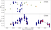 |
Fig. 1. Upper panel: SMW index variation of ζ1 Ret. HARPS data are indicated with blue circles (for both panels), while REOSC and FEROS data are indicated with green triangles and orange squares, respectively. Lower panel: activity variation for ζ2 Ret. Here, UVES data are indicated with black diamonds. Both vertical dashed lines in each panel represent the time coverage of those series that were initially reported, while the new data are indicated with red crosses. Red and black dashed lines show the fitted activity maxima f(t) for both peaks. |
A direct comparison of these new time series shows a clear decrease in the amplitude of the chromospheric activity of the ζ2 Ret component (from the first peak to the last one). To quantify this decrease in activity, in Fig. 1 we fitted the corresponding time series assuming a typical solar activity shape f(t) for each peak (see Eq. (8) in Egeland et al. 2017, for more details). The first cycle fit (red dashed line) is given by the following parameters: A = 0.0104, B = 1.32 yr, α = −0.24 yr−2, tm = 2008.67 yr (xJD = 4711.72 days), and fmin = 0.17422, while the corresponding parameters for the second cycle (black dashed line) are A = 0.0053, B = 1.59 yr, α ∼ 2 × 10⁻²⁶ yr−2, tm = 2016.42 yr (xJD = 7542.22 days), and fmin = 0.1746. As a result, both fits show an amplitude of ΔSMW = 0.0084 and ΔSMW = 0.0045, meaning a decrease of ∼47% in the activity cycle amplitude. To classify each component according to their variability type, we considered the criteria adopted by Baliunas et al. (1995). Then, ζ1 Ret can be classified as a variable star (with σS/ ∼ 4.3%), while ζ2 Ret would be classified as a ‘flat star’ (σS/
 ∼ 1.4%), although its stellar activity shows a clear variation. For comparative purposes, we also computed the log
  index by subtracting the photospheric contribution following the prescription given in Noyes et al. (1984), resulting in a mean activity difference of ∼0.24 dex, which is slightly higher than the previous value of 0.22 dex reported in Flores et al. (2018a).
In order to explore the components of the Ca II H&K line-core fluxes responsible for the low SMW index in ζ2-pagination Ret, we computed its basal level of activity. Schrijver et al. (1989) concluded that the line-core emission in the Ca II lines is composed by a photospheric component, a basal flux probably related to acoustic heating, and a third component associated with purely magnetic activity. In this sense, we estimated the Ca II photospheric component using a synthetic spectra calculated with SYNTHE and ATLAS9 model atmospheres (Kurucz 1993), accounting for a photospheric Mount Wilson index of SPhot = 0.149. Following Mittag et al. (2013), we converted this index to the Ca II line-core photospheric fluxes of (2.539 ± 0.017) × 106 erg cm−2 s−1, which are higher than the photospheric flux derived in Noyes et al. (1984) for a star of B − V = 0.60. Mittag et al. (2013) revised this historical work and determined that the photospheric flux was underestimated. They also computed an excess basal flux non-photospheric in erg cm−2 s−1 given by  . Considering this contribution,
  erg cm−2 s−1 and the photospheric flux derived from Sphot for ζ2 Ret, the entire basal contribution
  erg cm−2 s−1 is associated to a Mount Wilson index of SMW ∼ 0.180. The mean activity level of ζ2 Ret between 6658.5 and 8849.5 days is slightly lower in less than 1.5σ, thus it is mainly related to a basal chromospheric heating. Although a remaining magnetic contribution is still evident in the activity cycle.
To search for long-term activity cycles in this binary system, we first calculated the monthly means of all data. This procedure, which has been applied in previous works (e.g. Baliunas et al. 1995; Metcalfe et al. 2010; Gomes da Silva et al. 2011; Flores et al. 2018b), enables us to reduce the rotational scatter originated by individual active regions. Following Zechmeister & Kürster (2009), we computed the Generalised Lomb-Scargle periodogram (hereafter GLS) and the false-alarm probability (hereafter FAP, see their equation 24) of each significant peak present in the periodograms. In the upper and lower panels of Fig. 2, we show the GLS (blue dashed line) for ζ1-pagination Ret and ζ2 Ret, respectively. Both stars seem to be periodic. In the case of ζ1, we found two prominent peaks which can be associated with activity cycles, one of them has a period of 1548 ± 62 d with an FAP of 1 × 10⁻¹⁴. While, the second peak is 431 ± 6 d with an FAP of 2 × 10−08. For the ζ2 Ret component, the large data set collected in this work allowed us to re-calculate its previously reported period (3670 ± 170 d). A prominent peak of 3047 ± 134 d with an FAP of 4 × 10⁻¹² was detected in the GLS periodogram (see the lower panel of Fig. 2). Therefore, ζ2 Ret also satisfies the Baliunas et al. (1995) criteria for a cycling star (i.e. FAP ≤ 10−02).
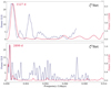 |
Fig. 2. GLS (blue dashed line) and CLEAN (red continuous line) periodograms for the means of the Mount Wilson indexes plotted in Fig. 1. Upper and lower panels: correspond to ζ1 Ret and ζ2 Ret, respectively. The most significant CLEAN periods are indicated in each panel. |
We also executed the CLEAN deconvolution algorithm (Roberts et al. 1987) to explore whether the 431 day period which appears in the GLS periodogram of ζ1 Ret is due to sampling. A comparison between GLS (blue dashed line) and CLEAN (red continuous line) periodograms is shown in Fig. 2. For the case of ζ1, we found that the only predominant peak is around 1527 ± 43 d, while for ζ2 we obtained a single significant period of 2899 ± 139 d. The errors of the periods detected with the CLEAN algorithm depend on the finite frequency resolution of the periodograms δν as given by Eq. (2) in Lamm et al. (2004),  . Therefore, the periods found for the binary system employing the CLEAN algorithm correspond to those associated with the GLS method.
Finally, in Fig. 3 we show the monthly average values of the SMW index for ζ2 Ret phased with the period derived with the CLEAN algorithm. The errors of these data were calculated as their standard deviation; whereas for those bins with a single measurement, we considered the typical dispersion of other bins.
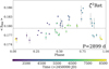 |
Fig. 3. Monthly means of the Mount Wilson indexes for ζ2 Ret phased with a period of ∼7.9 yr. The observing seasons are represented by coloured circles. The error bars of HARPS data and the corresponding mean activity level (dashed horizontal line) have been included. |
4. Discussion and conclusions
Following the aim of this study, we carried out a long-term activity of the ζ Ret binary system employing several spectroscopic data obtained over a span of 19 years. We detected long-term activity cycles of 1527 ∼ 43 d (∼4.2 yr, not yet reported in the literature) and 2899 ∼ 139 d (∼7.9 yr) for ζ1 and ζ2 Ret, respectively. In particular, the new data included in this work allowed us to make a better estimation for the period obtained in Flores et al. (2018a) for ζ2 Ret.
Flores et al. (2018a) propose two possible scenarios to explain the large difference in activity between the stars ζ1 and ζ2 Ret. In the first scenario, the stars possibly present different rotational periods9, which could result in different average activity levels. The second scenario suggests that the star ζ2 Ret is possibly in an MM state. In the present work we collected new evidence, including more than 430 spectra acquired with the HARPS, REOSC, FEROS, and UVES spectrographs, which support the idea that ζ2 Ret is possibly in an MM state due to the following reasons.
-
There is a large difference in the average activity levels between both stars (hereafter Δ). DO98 and Wright (2004) suggested that binary systems, presumably co-eval stars, with significant Δ levels could point to an MM state of the most inactive star. In particular, DO98 suggest that an age difference (estimated using an activity-age calibration) greater than ∼1 Gyr could indicate an MM state. Using the DO98 calibration, we estimate ages of 1.5 and 3.3 Gyr for ζ1 Ret and ζ2 Ret, that is to say a notable difference of ∼1.8 Gyr. An age difference greater than 1.0 Gyr is also obtained through the Mamajek & Hillenbrand (2008) and Lorenzo-Oliveira et al. (2016) calibrations.
-
In fact, the value of Δ = 0.24 dex we found in the present work for most recent years has increased from the value Δ = 0.22 dex reported in Flores et al. (2018a).
-
The cycle amplitude of ζ2 Ret decreased notably, from ΔSMW = 0.0084 to ΔSMW = 0.0045 in the last cycle, that is to say it decreased by ∼47%. We caution that, until now, there is no clear agreement about the solar cycle behaviour during the MM state. Initially, sunspot records suggested that the cycle was interrupted (e.g. Spoerer & Maunder 1890; Eddy 1976; Wilson 1994). However, different works using counts of sunspots and cosmogenic isotopes indicate a weaker but persistent cycle (e.g. Ribes & Nesme-Ribes 1993; Beer et al. 1998; Miyahara et al. 2004; Poluianov et al. 2014; Vaquero et al. 2015). In addition to the Sun, Shah et al. (2018) show that the G5V star HD 4915, which is a candidate to present an MM state, also reveals a cycle still in progress with decreasing amplitude, similar to ζ2 Ret.
-
The current activity level of ζ2 Ret is very low (⟨FHK⟩∼3 × 10⁶ erg cm−2 s−1). This value is even lower within the statistical error than the theoretical basal level for this object (FHK = (3.10 ± 0.07)×106 erg cm−2 s−1). The basal value was determined by estimating the sum of the non-photospheric basal flux
 for B − V = 0.60 (Mittag et al. 2013), and the photospheric contribution was estimated using a synthetic spectra calculated with SYNTHE and ATLAS9 model atmospheres (Kurucz 1993). The stellar parameters of ζ2 Ret were taken from the high-precision analysis of Saffe et al. (2016).
Finding an unambiguous example of an MM candidate is a very difficult task, which is due in part to the fact that an MM state in general is not totally clear, and it requires a large observational time span. To date, only very few MM candidates have been reported in the literature, HD 4915 being one of them (Shah et al. 2018). For the case of ζ2 Ret, we profit from the fact that this star belongs to a binary system, which makes it a very valuable candidate. In fact, to our knowledge, ζ2 Ret is the first MM candidate to have been detected through the activity differences in a binary system, as suggested by DO98.
Finally, we strongly recommend searching for valuable MM candidates in those binary systems with high activity differences. They can be used as good laboratories to address many questions related to solar and stellar MM, which have yet to be subjected to intense scrutiny (see Zolotova & Ponyavin 2015; Vaquero et al. 2015; Carrasco et al. 2019, for more details).
While those stars with an σS/ ≥ 2% are considered variable or erratic.
The main aim of the HKα project consists in the systematic observation of main sequence stars to carry out long-term activity studies (see Cincunegui & Mauas 2004, for more details).
IRAF is distributed by the National Optical Astronomical Observatories, which is operated by the Association of Universities for Research in Astronomy, Inc. (AURA), under a cooperative agreement with the National Science Foundation.
The analysis of these new spectroscopic data does not reveal the presence of any reliable rotational modulation for both stars.
Acknowledgments
We warmly thank the anonymous referee for constructive comments that improved the Letter. MF, MJA, RIB, NN, and PM acknowledge the financial support of PROJOVI/UNSJ, through the project 80020190300048SJ. Also, RIB, JA, and PM acknowledge the financial support from CONICET in the forms of doctoral and post-doctoral fellowships. JYG acknowledges the support from CNPq.
References
- Baliunas, S., & Jastrow, R. 1990, Nature, 348, 520 [NASA ADS] [CrossRef] [Google Scholar]
- Baliunas, S. L., Donahue, R. A., Soon, W. H., et al. 1995, ApJ, 438, 269 [NASA ADS] [CrossRef] [Google Scholar]
- Baliunas, S. L., Donahue, R. A., Soon, W., & Henry, G. W. 1998, ASP Conf. Ser., 154, 153 [Google Scholar]
- Beer, J., Tobias, S., & Weiss, N. 1998, Sol. Phys., 181, 237 [Google Scholar]
- Carrasco, V. M. S., Vaquero, J. M., Gallego, M. C., et al. 2019, ApJ, 886, 18 [CrossRef] [Google Scholar]
- Charbonneau, P. 2010, Liv. Rev. Sol. Phys., 7, 3 [Google Scholar]
- Cincunegui, C., & Mauas, P. J. D. 2004, A&A, 414, 699 [NASA ADS] [CrossRef] [EDP Sciences] [Google Scholar]
- Cincunegui, C., Díaz, R. F., & Mauas, P. J. D. 2007, A&A, 469, 309 [NASA ADS] [CrossRef] [EDP Sciences] [Google Scholar]
- Donahue, R. A. 1998, in Cool Stars, Stellar Systems, and the Sun, eds. R. A. Donahue, & J. A. Bookbinder, ASP Conf. Ser., 154, 1235 [Google Scholar]
- Eddy, J. A. 1976, Science, 192, 1189 [NASA ADS] [CrossRef] [PubMed] [Google Scholar]
- Egeland, R., Soon, W., Baliunas, S., et al. 2017, ApJ, 835, 25 [NASA ADS] [CrossRef] [Google Scholar]
- Flores, M., Saffe, C., Buccino, A., et al. 2018a, MNRAS, 476, 2751 [NASA ADS] [CrossRef] [Google Scholar]
- Flores, M., González, J. F., Jaque Arancibia, M., et al. 2018b, A&A, 620, A34 [NASA ADS] [CrossRef] [EDP Sciences] [Google Scholar]
- Giampapa, M. S. 2012, in IAU Symposium, eds. C. H. Mandrini, & D. F. Webb, 286, 257 [Google Scholar]
- Gomes da Silva, J., Santos, N. C., Bonfils, X., et al. 2011, A&A, 534, A30 [NASA ADS] [CrossRef] [EDP Sciences] [Google Scholar]
- Henry, T. J., Soderblom, D. R., Donahue, R. A., & Baliunas, S. L. 1996, AJ, 111, 439 [NASA ADS] [CrossRef] [Google Scholar]
- Jenkins, J. S., Jones, H. R. A., Pavlenko, Y., et al. 2008, A&A, 485, 571 [NASA ADS] [CrossRef] [EDP Sciences] [Google Scholar]
- Judge, P. G., & Saar, S. H. 2007, ApJ, 663, 643 [NASA ADS] [CrossRef] [Google Scholar]
- Kurucz, R. 1993, ATLAS9 Stellar Atmosphere Programs and 2 km/s Grid (Cambridge, Mass.: Smithsonian Astrophysical Observatory), 13 [Google Scholar]
- Lamm, M. H., Bailer-Jones, C. A. L., Mundt, R., Herbst, W., & Scholz, A. 2004, A&A, 417, 557 [NASA ADS] [CrossRef] [EDP Sciences] [Google Scholar]
- Lorenzo-Oliveira, D., Porto de Mello, G. F., & Schiavon, R. P. 2016, A&A, 594, L3 [NASA ADS] [CrossRef] [EDP Sciences] [Google Scholar]
- Lovis, C., Dumusque, X., Santos, N. C., et al. 2011, ArXiv e-prints [arXiv:1107.5325] [Google Scholar]
- Mamajek, E. E., & Hillenbrand, L. A. 2008, ApJ, 687, 1264 [NASA ADS] [CrossRef] [Google Scholar]
- Metcalfe, T. S., Basu, S., Henry, T. J., et al. 2010, ApJ, 723, L213 [NASA ADS] [CrossRef] [Google Scholar]
- Mittag, M., Schmitt, J. H. M. M., & Schröder, K. P. 2013, A&A, 549, A117 [NASA ADS] [CrossRef] [EDP Sciences] [Google Scholar]
- Miyahara, H., Masuda, K., Muraki, Y., et al. 2004, Sol. Phys., 224, 317 [Google Scholar]
- Nagovitsyn, Y. A. 2007, Astron. Lett., 33, 340 [NASA ADS] [CrossRef] [Google Scholar]
- Noyes, R. W., Hartmann, L. W., Baliunas, S. L., Duncan, D. K., & Vaughan, A. H. 1984, ApJ, 279, 763 [NASA ADS] [CrossRef] [Google Scholar]
- Poluianov, S. V., Usoskin, I. G., & Kovaltsov, G. A. 2014, Sol. Phys., 289, 4701 [Google Scholar]
- Poppenhäger, K., Robrade, J., Schmitt, J. H. M. M., & Hall, J. C. 2009, A&A, 508, 1417 [NASA ADS] [CrossRef] [EDP Sciences] [Google Scholar]
- Ribes, J. C., & Nesme-Ribes, E. 1993, A&A, 276, 549 [NASA ADS] [Google Scholar]
- Ribes, E., Merlin, P., Ribes, J. C., & Barthalot, R. 1989, Ann. Geophys., 7, 321 [Google Scholar]
- Roberts, D. H., Lehar, J., & Dreher, J. W. 1987, AJ, 93, 968 [Google Scholar]
- Saar, S. H., & Baliunas, S. L. 1992, in The Solar Cycle, ed. K. L. Harvey, ASP Conf. Ser., 27, 150 [Google Scholar]
- Saffe, C., Flores, M., Jaque Arancibia, M., Buccino, A., & Jofré, E. 2016, A&A, 588, A81 [NASA ADS] [CrossRef] [EDP Sciences] [Google Scholar]
- Schrijver, C. J., Dobson, A. K., & Radick, R. R. 1989, ApJ, 341, 1035 [NASA ADS] [CrossRef] [Google Scholar]
- Schröder, K. P., Mittag, M., Schmitt, J. H. M. M., et al. 2017, MNRAS, 470, 276 [CrossRef] [Google Scholar]
- Shah, S. P., Wright, J. T., Isaacson, H., Howard, A. W., & Curtis, J. L. 2018, ApJ, 863, L26 [CrossRef] [Google Scholar]
- Shaya, E. J., & Olling, R. P. 2011, ApJS, 192, 2 [NASA ADS] [CrossRef] [Google Scholar]
- Soon, W. W. H., & Yaskell, S. H. 2003, The Maunder Minimum and the Variable Sun-Earth Connection (Singapore: World Scientific Publ. C) [CrossRef] [Google Scholar]
- Spoerer, F. W. G., & Maunder, E. W. 1890, MNRAS, 50, 251 [Google Scholar]
- Usoskin, I. G., Mursula, K., & Kovaltsov, G. A. 2001, J. Geophys. Res., 106, 16039 [Google Scholar]
- Usoskin, I. G., Solanki, S. K., Taricco, C., Bhandari, N., & Kovaltsov, G. A. 2006, A&A, 457, L25 [NASA ADS] [CrossRef] [EDP Sciences] [Google Scholar]
- Vaquero, J. M., Kovaltsov, G. A., Usoskin, I. G., Carrasco, V. M. S., & Gallego, M. C. 2015, A&A, 577, A71 [NASA ADS] [CrossRef] [EDP Sciences] [Google Scholar]
- Vaughan, A. H., Preston, G. W., & Wilson, O. C. 1978, PASP, 90, 267 [NASA ADS] [CrossRef] [Google Scholar]
- Wilson, O. C. 1978, ApJ, 226, 379 [NASA ADS] [CrossRef] [Google Scholar]
- Wilson, P. R. 1994, Cambridge Astrophysics Series (New York: Cambridge University Press), 24 [Google Scholar]
- Wright, J. T. 2004, AJ, 128, 1273 [NASA ADS] [CrossRef] [Google Scholar]
- Zechmeister, M., & Kürster, M. 2009, A&A, 496, 577 [NASA ADS] [CrossRef] [EDP Sciences] [Google Scholar]
- Zolotova, N. V., & Ponyavin, D. I. 2015, ApJ, 800, 42 [NASA ADS] [CrossRef] [Google Scholar]
Appendix A: Observational data and derived Mount Wilson indexes for ζ Ret
The tables are available at the CDS.
All Figures
|
Fig. 1. Upper panel: SMW index variation of ζ1 Ret. HARPS data are indicated with blue circles (for both panels), while REOSC and FEROS data are indicated with green triangles and orange squares, respectively. Lower panel: activity variation for ζ2 Ret. Here, UVES data are indicated with black diamonds. Both vertical dashed lines in each panel represent the time coverage of those series that were initially reported, while the new data are indicated with red crosses. Red and black dashed lines show the fitted activity maxima f(t) for both peaks. |
| In the text | |
|
Fig. 2. GLS (blue dashed line) and CLEAN (red continuous line) periodograms for the means of the Mount Wilson indexes plotted in Fig. 1. Upper and lower panels: correspond to ζ1 Ret and ζ2 Ret, respectively. The most significant CLEAN periods are indicated in each panel. |
| In the text | |
|
Fig. 3. Monthly means of the Mount Wilson indexes for ζ2 Ret phased with a period of ∼7.9 yr. The observing seasons are represented by coloured circles. The error bars of HARPS data and the corresponding mean activity level (dashed horizontal line) have been included. |
| In the text | |
Current usage metrics show cumulative count of Article Views (full-text article views including HTML views, PDF and ePub downloads, according to the available data) and Abstracts Views on Vision4Press platform.
Data correspond to usage on the plateform after 2015. The current usage metrics is available 48-96 hours after online publication and is updated daily on week days.
Initial download of the metrics may take a while.