| Issue |
A&A
Volume 645, January 2021
|
|
|---|---|---|
| Article Number | A22 | |
| Number of page(s) | 10 | |
| Section | Planets and planetary systems | |
| DOI | https://doi.org/10.1051/0004-6361/202039302 | |
| Published online | 22 December 2020 | |
Detection of the hydrogen Balmer lines in the ultra-hot Jupiter WASP-33b
1
Institut für Astrophysik, Georg-August-Universität,
Friedrich-Hund-Platz 1,
37077
Göttingen, Germany
e-mail: This email address is being protected from spambots. You need JavaScript enabled to view it.
2
Université Grenoble Alpes, CNRS, IPAG,
38000
Grenoble, France
3
Instituto de Astrofísica de Canarias (IAC),
Calle Vía Lactea s/n,
38200
La Laguna,
Tenerife, Spain
4
Departamento de Astrofísica, Universidad de La Laguna,
38026
La Laguna,
Tenerife, Spain
5
Max-Planck-Institut für Astronomie,
Königstuhl 17,
69117
Heidelberg, Germany
6
Hamburger Sternwarte, Universität Hamburg,
Gojenbergsweg 112,
21029
Hamburg, Germany
7
Landessternwarte, Zentrum für Astronomie der Universität Heidelberg,
Königstuhl 12,
69117
Heidelberg, Germany
8
Key Laboratory of Planetary Sciences, Purple Mountain Observatory, Chinese Academy of Sciences,
Nanjing
210023, PR China
9
Leiden Observatory, Leiden University,
Postbus 9513,
2300 RA,
Leiden, The Netherlands
10
Lunar and Planetary Laboratory, 1629 E. University Blvd.,
PO Box 210092,
Tucson,
AZ 85721-0092, USA
11
Institut de Ciències de l’Espai (CSIC-IEEC),
Campus UAB, c/ de Can Magrans s/n,
08193
Bellaterra,
Barcelona, Spain
12
Institut d’Estudis Espacials de Catalunya (IEEC),
08034
Barcelona, Spain
13
Centro de Astrobiología (CSIC-INTA), ESAC, Camino bajo del castillo s/n,
28692
Villanueva de la Cañada,
Madrid, Spain
14
Instituto de Astrofísica de Andalucía (IAA-CSIC),
Glorieta de la Astronomía s/n,
18008
Granada, Spain
15
Universidad Complutense de Madrid, Departamento de Física de la Tierra y Astrofísica and IPARCOS-UCM (Instituto de Física de Partículas y del Cosmos de la UCM),
Facultad de Ciencias Físicas,
28040
Madrid, Spain
16
Thüringer Landessternwarte Tautenburg,
Sternwarte 5,
07778
Tautenburg, Germany
17
Centro Astronónomico Hispano-Alemán (CSIC-MPG), Observatorio Astronónomico de Calar Alto, Sierra de los Filabres,
04550
Gérgal,
Almería, Spain
Received:
31
August
2020
Accepted:
15
November
2020
Abstract
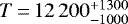
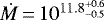
Ultra-hot Jupiters (UHJs) are highly irradiated giant exoplanets with extremely high day-side temperatures, which lead to thermal dissociation of most molecular species. It is expected that the neutral hydrogen atom is one of the main species in the upper atmospheres of UHJs. Neutral hydrogen has been detected in several UHJs by observing their Balmer line absorption. In this work, we report four transit observations of the UHJ WASP-33b, performed with the CARMENES and HARPS-North spectrographs, and the detection of the Hα, Hβ, and Hγ lines in the planetary transmission spectrum. The combined Hα transmission spectrum of the four transits has an absorption depth of 0.99 ± 0.05%, which corresponds to an effective radius of 1.31 ± 0.01 Rp. The strong Hα absorption indicates that the line probes the high-altitude thermosphere. We further fitted the three Balmer lines using the PAWN model, assuming that the atmosphere is hydrodynamic and in local thermodynamic equilibrium. We retrieved a thermosphere temperature 12 200−1000+1300 K and a mass-loss rate Ṁ = 1011.8−0.5+0.6 g s−1. The retrieved high mass-loss rate is compatible with the “Balmer-driven” atmospheric escape scenario, in which the stellar Balmer continua radiation in the near-ultraviolet is substantially absorbed by excited hydrogen atoms in the planetary thermosphere.
Key words: planets and satellites: atmospheres / techniques: spectroscopic / planets and satellites: individual: WASP-33b
© ESO 2020
1 Introduction
Ultra-hot Jupiters (UHJs) are the hottest giant exoplanets and they are extensively irradiated by their host stars. These planets are ideal laboratories to study the chemistry and physics of planetary atmospheres under extreme conditions. Theoretical modelling of UHJ atmospheres (e.g. Lothringer et al. 2018; Parmentier et al. 2018; Kitzmann et al. 2018; Helling et al. 2019) suggests that the day-sides as well as the terminators of UHJs are extremely hot and probably dominated by atoms and ions instead of molecules as a result of thermal dissociation and ionisation.
Thermal emission spectra of several UHJs, including HAT-P-7b (Mansfield et al. 2018), WASP-12b (Stevenson et al. 2014), WASP-18b (Arcangeli et al. 2018), and WASP-103b (Kreidberg et al. 2018), have been observed with the Hubble Space Telescope (HST). These thermal spectra exhibit a lack of H2 O features, which is probably due to thermal dissociation (Parmentier et al. 2018). On the other hand, emission spectroscopy with high-resolution spectrographs has revealed the existence of neutral Fe in KELT-9 (Pino et al. 2020), WASP-189b (Yan et al. 2020), and WASP-33b (Nugroho et al. 2020a). In addition to the thermal emission spectra, phase curve observations have been performed for several UHJs, including WASP-33b (Zhang et al. 2018; von Essen et al. 2020), WASP-121b (Daylan et al. 2019; Bourrier et al. 2020a), and KELT-9b (Wong et al. 2020; Mansfield et al. 2020). These observations suggest that these UHJs have relatively low day-night temperature contrasts and relatively high heat transport efficiencies. The increased heat transport efficiency in UHJs could be explained by a new physical mechanism – thermal dissociation and recombination of H2 (Bell & Cowan 2018; Komacek & Tan 2018).
Transmission spectroscopy has also been widely used in probing the atmospheres of UHJs, and various atomic and ionic species havebeen detected. In the atmosphere of KELT-9b, the hottest exoplanet discovered so far, hydrogen Balmer lines as well as multiple metal lines (including Fe I, Fe II, Ti II, Mg I, and Ca II) have been detected (Yan & Henning 2018; Hoeijmakers et al. 2018, 2019; Cauley et al. 2019; Yan et al. 2019; Turner et al. 2020). Various metals as well as Balmer lines have been detected in KELT-20b/MASCARA-2b (Casasayas-Barris et al. 2018, 2019; Stangret et al. 2020; Nugroho et al. 2020b; Hoeijmakers et al. 2020). Ca II has been detected in WASP-33b (Yan et al. 2019). Balmer lines and metals including Na I, Mg II, Fe I, Fe II, Cr I, and V I have been detected in WASP-121b(Sing et al. 2019; Bourrier et al. 2020b; Gibson et al. 2020; Cabot et al. 2020; Ben-Yami et al. 2020). Hα and Mg II have been discovered in WASP-12b (Fossati et al. 2010; Jensen et al. 2018). Neutral Fe has also been detected at the terminator of WASP-76b (Ehrenreich et al. 2020).
Planets experiencing strong stellar irradiation are thought to undergo hydrodynamic atmospheric escape (e.g. Owen 2019, and references therein). The hydrodynamic escape in hydrogen-dominated atmospheres is normally driven by the absorption of stellar extreme-ultraviolet (EUV) flux (Yelle 2004; Tian et al. 2005; Salz et al. 2016). However, Fossati et al. (2018) found that heating due to atomic absorption of the stellar UV and optical flux drives the atmosphericescape of UHJs orbiting early-type stars. García Muñoz & Schneider (2019) further proposed that the absorption of the hydrogen Balmer line series can enhance and even drive the atmospheric escape of UHJs orbiting hot stars.
Observations of atmospheric escape have been performed with the hydrogen Lyα line (Vidal-Madjar et al. 2003; Lecavelier des Etangs et al. 2012; Ehrenreich et al. 2015) as well as metal lines in the ultraviolet (Fossati et al. 2010; Sing et al. 2019; Cubillos et al. 2020), using the Space Telescope Imaging Spectrograph on HST. The helium 10 833 Å line has recently been used in probing escaping atmosphere of planets orbiting active stars (e.g. Spake et al. 2018; Nortmann et al. 2018; Allart et al. 2018; Salz et al. 2018; Lampón et al. 2020; Palle et al. 2020).
Hydrogen Balmer lines can also be used to probe high-altitude atmospheres and study atmospheric escape. For example, Yan & Henning (2018) estimated the Jeans escape rate of KELT-9b with the Hα absorption line. Recently, Wyttenbach et al. (2020) modelled Balmer lines with a hydrodynamic model and retrieved the mass-loss rate of KELT-9b. Balmer lines have been detected in four UHJs so far: KELT-9b (Yan & Henning 2018; Cauley et al. 2019; Turner et al. 2020), KELT-20b (Casasayas-Barris et al. 2018, 2019), WASP-12b (Jensen et al. 2018), and WASP-121b (Cabot et al. 2020). Besides, the Hα line has been detected in two non-UHJ planets – HD 189733b (Jensen et al. 2012; Barnes et al. 2016; Cauley et al. 2016, 2017a,b) and WASP-52b (Chen et al. 2020). The Hα absorption in these two planets probably originates from the excitation of hydrogen atoms due to stellar Lyα line and Lyman continuum irradiation (Christie et al. 2013; Huang et al. 2017).
In this work, we present the discovery of Balmer line absorption during the transit of WASP-33b – a UHJ (equilibrium temperature ~2710 K) orbiting an A5 star (Collier Cameron et al. 2010). Several species have previously been detected in its planetary atmosphere, including TiO (Haynes et al. 2015; Nugroho et al. 2017), Ca II (Yan et al. 2019), Fe I (Nugroho et al. 2020a), and evidence of AlO (von Essen et al. 2019) and FeH (Kesseli et al. 2020). The paper is organised as follows. We describe the transit observations and data analysis in Sect. 2. The observational results are presented in Sect. 3. In Sect. 3.3, we present a hydrodynamic model of the Balmer lines and discuss the atmospheric escape of WASP-33b. The conclusions are summarised in Sect. 4.
2 Data and analysis
2.1 Observations
We observed four transits of WASP-33b with two spectrographs. The observation logs are summarised in Table 1. Two transits were observed with the CARMENES (Quirrenbach et al. 2018) installed at the 3.5 m telescope of the Calar Alto Observatoryon 5 January 2017 and 16 January 2017. The visual channel of the CARMENES spectrograph has a resolution of R ~94 600 and a wavelength coverage of 520–960 nm. The first night was photometric (i.e. ideal weather condition during the observation) and the second night was partially cloudy.
Another two transits were observed with the HARPS-North (HARPS-N) spectrograph mounted on the Telescopio Nazionale Galileo telescope on 17 October 2018 and 8 November 2018. The instrument has a resolution of R ~115 000 and a wavelength coverage of 383–690 nm. We used the order-merged one-dimensional spectra from the HARPS-N pipeline (Data Reduction Software). The spectra have an over-sampled wavelength step of 0.01 Å. We re-binned the spectrum every three wavelength points by averaging so that each wavelength point corresponds to 0.03 Å, which is similar to the CARMENES pixel size at the Hα line centre (0.030 Å). Both nights were photometric. However, the spectral flux from the first night observation had a large drop when the telescope was pointing close to the zenith. Such a phenomenon also occurred during transit observations in Casasayas-Barris et al. (2019), which was probably caused by a problem with the atmospheric dispersion corrector (ADC).
The signal-to-noise ratio (S/N) per wavelength point (~0.03 Å) at the Hα line centre is plotted in Fig. 1. Among the four transits, night-1 from CARMENES and night-2 from HARPS-N observationshave much higher S/N and, therefore, were used in Yan et al. (2019) for the detection of ionised calcium. In this work, we use and combine all four transits.
2.2 Obtaining the transmission spectral matrix
We investigated the Hα line (6562.79 Å) using both the CARMENES and HARPS-N observations and the Hβ (4861.35 Å) and Hγ (4340.47 Å) lines from the HARPS-N observations. The data reduction method is similar to the method in Yan & Henning (2018).
The spectra were first normalised and shifted into the Earth’s rest frame. We then removed the telluric absorption lines using a theoreticaltransmission spectral model of the Earth’s atmosphere (Yan et al. 2015a). The spectra were subsequently aligned into the stellar rest frame by correcting the barycentric radial velocity (RV) and the stellar systemic velocity (−3.0 km s−1, Nugroho et al. 2017). We obtained an out-of-transit master spectrum by adding up all the out-of-transit spectra with the squared S/N as weight. We then divided each spectrum by the master spectrum to remove the stellar lines. The residual spectrum was subsequently filtered with a Gaussian high-pass filter (σ ~ 300 points) to remove large-scale features on the continuum spectrum, which may be attributed to the stability of the HARPS-N ADC, stellar pulsation, or the imperfect normalisation of the blaze variation.
We combined the two CARMENES observations as well as the two HARPS-N observations by binning the spectra with an orbital phase step of 0.005. The binning was performed by averaging the spectra within each phase bin with the squared S/N as weight.
By applying these procedures, we obtained a transmission spectral matrix for each of the Hα, Hβ, and Hγ lines from the HARPS-N observationsand an Hα spectral matrix from the CARMENES observations (upper panels in Figs. 2 and 3).
Observation logs.
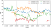 |
Fig. 1 Signal-to-noise ratio per wavelength point (~0.03 Å) at the Hα line centre. The dashed lines indicate the beginning and end of transit. |
2.3 Model of stellar RM and CLV effects
The stellar line profile varies during the transit due to the Rossiter-McLaughlin (RM) effect (Queloz et al. 2000) and the centre-to-limb variation (CLV) effect (Yan et al. 2015b, 2017; Czesla et al. 2015). We modelled the RM and CLV effects simultaneously following the method described in Yan & Henning (2018). We used the same stellar and planetary parameters as in Yan et al. (2019).
The planetary orbit of WASP-33b undergoes a nodal precession (Johnson et al. 2015; Iorio 2016; Watanabe et al. 2020). We adoptedthe orbital change rates from Johnson et al. (2015) and calculated the expected orbital inclination (i) and spin-orbit angle (λ) at the dates of our observations. Because the observation dates are very close for the two CARMENES transits as well as for the two HARPS-N transits, the changes of the orbital parameters between them are negligible. Therefore, we set i = 89.50 deg and λ = − 114.05 deg for the combined CARMENES transmission matrix; i = 90.14 deg and λ = −114.93 deg for the combined HARPS-N transmission matrix.
2.4 Fitting the observed spectral matrix
We fitted the observed transmission spectral matrix with a model consisting of two components: the planetary absorption and the stellar line profile change. We assumed that the planetary absorption has a Gaussian profile described by the full width at half maximum (FWHM), the absorption depth (h), and the RVshift of the observed line centre compared to the theoretical value (Vcentre). The semi-amplitude of the planetary orbital motion (Kp) is fixed to the expected Kp value (231 ± 3 km s−1), which is calculated with the planetary orbital parameters. The stellar line profile change caused by the RM and CLV effects is fixed to the results as calculated in Sect. 2.3.
We sampled from the posterior probability distribution using the Markov chain Monte Carlo (MCMC) simulations with the emcee tool (Foreman-Mackey et al. 2013). We only used the fully in-transit data (i.e. excluding the ingress and egress phases).
3 Results and discussion
3.1 Hα transmission spectrum
The transmission spectral matrices are shown in Fig. 2a. The Hα absorption is clearly detected in both CARMENES and HARPS-N data. The best-fit models of the planetary absorption feature as well as the stellar CLV and RM effects are shown in Fig. 2b, and the best-fit parameters are summarised in Table 2. To obtain the one-dimensional transmission spectra, we firstly corrected the CLV and RM effects. Then, the residual spectra were shifted into the planetary rest frame. We subsequently averaged all the fully in-transit spectra to derive the final one-dimensional transmission spectra, which are presented in Fig. 4. The Hα transmission spectrum of each night is shown in Fig. A.1.
The obtained FWHM is 31.6 km s−1 for HARPS-N and 35.6
 km s−1 for CARMENES. These values are lower than those of KELT-9b (Yan & Henning 2018; Cauley et al. 2019; Turner et al. 2020), while slightly higher than those of KELT-20b (Casasayas-Barris et al. 2018, 2019). The large FWHM indicates that the Hα absorption is optically thick (Huang et al. 2017).
The measured RV shift of the line centre is 2.0 ± 1.9 km s−1 for HARPS-N and 0.8 ± 1.1 km s−1 for CARMENES. The RV shift has been used to measure high-altitude winds at the planetary terminator (Snellen et al. 2010; Wyttenbach et al. 2015; Louden & Wheatley 2015; Brogi et al. 2016). Nevertheless, the measured Vcentre is relative to the stellar systemic RV and there is a large uncertainty of the stellar RV of WASP-33. This is because precisely measuring absolute RVs of fast-rotating A-type stars is intrinsically challenging. For example, the reported systemic RVs of WASP-33 deviate by several km s−1 (Collier Cameron et al. 2010; Lehmann et al. 2015; Nugroho et al. 2017; Cauley et al. 2020a). Therefore, we conclude that we do not detect any significant winds at the terminator of WASP-33b considering the uncertainties in the measured Vcentre values and the stellar systemic RV.
We further combined the CARMENES and HARPS-N transmission spectral matrices using the binning method as described in Sect. 2.2. The stellar CLV and RM effects were already corrected before the averaging. The combined matrix is presented in Fig. 5 and the best-fit parameters are listed in Table 2. We calculated the equivalent width of the absorption line (WHα) using the same method as in Yan & Henning (2018), except that the integration range was set as ± 35 km s−1 to match the observed FWHM. Figure 6 shows the time series of WHα. There is no obvious pre- or after-transit absorption, although the absorption depth is slightly stronger during the first-half transit.
In general, the fitted parameters between CARMENES and HARPS-N are consistent. However, the CARMENES Hα absorption is somewhat stronger than the HARPS-N absorption. Such a slight difference between the two instruments is also observed for the Hα line in KELT-20b (Casasayas-Barris et al. 2019) and KELT-9b (Yan & Henning 2018; Wyttenbach et al. 2020; Turner et al. 2020). Although the difference could be from random variations, there may also be systematic residuals, which could be due to instrumental effects (e.g. non-linearity and the stability of the HARPS-N ADC) or data reduction procedures (e.g. imperfect normalisation and removal of stellar and telluric lines).
For the case of WASP-33b, the slight difference between the CARMENES and HARPS-N results could be caused by the stellar pulsations, which can affect the stellar Hα line profile. The host star is a known δ Scuti star with pronounced pulsations (Collier Cameron et al. 2010; von Essen et al. 2014; Kovács et al. 2013). For the CARMENES spectrum in Fig. 4, there is a bump feature on the left of the planetary absorption line. A weaker bump feature is also present in the HARPS-N spectrum. Such a bump feature is also observed in the transmission spectrum of the Ca II infrared triplet lines (Yan et al. 2019), which are obtained using the same transit data as in this work. On the combined transmission spectral matrix in Fig. 5, there are bright stripes on the left and right sides of the planetary absorption signal and these stripes extend beyond the transit. These stripes are probably the stellar pulsation signatures, which generate the bump features as observed on the transmission spectra in Fig. 4. For individual CARMENES and HARPS-N observation, the position and strength of the pulsation features were not the same during the transits. Therefore, the stellar pulsation could introduce a difference between the CARMENES and HARPS-N results. In a preprint posted while the present paper was under review, Cauley et al. (2020a) reported the detection of the Balmer lines in WASP-33b using the PEPSI spectrograph mounted on the Large Binocular Telescope. Their obtained absorption line strength is quantitatively different but generally consistent with our CARMENES and HARPS-N results, considering possible effects of the stellar pulsation.
Although the detection of the Hα line is unambiguous, its strength is potentially affected by the stellar pulsation. To correct the effect of the pulsation, a detailed analysis of the variation in the stellar Balmer lines is required. Such an analysis requires data taken with high S/N and is beyond the scope of this paper. However, considering that the pulsating periods are not synchronous with the planetary orbital motion (von Essen et al. 2014), the pulsating contribution to the transmission spectrum should be statistically reduced when combining the four transit spectra together. To evaluate the effect of pulsation, we combined the out-of-transit spectra on the spectral matrix in Fig. 5 (i.e. phases –0.10 to –0.05 and +0.05 to +0.10) and assumed the in-transit orbital velocity to repeat during out-of-transit. The obtained out-of-transit spectrum (Fig. 7) shows ripple-like features with semi-amplitude of ~0.2%, which are most likely the results of the stellar pulsation. The effect of the pulsation to the Hα transmission spectrum should be at a similar order of these ripple features.
We note that Valyavin et al. (2018) analysed the transit light curve of WASP-33b observed with the Hα filter. These latter authors found that the Hα transit depth is significantly deeper than the transit depths measured in broad bands. Since we detect the strong Hα absorption line with high-resolution spectroscopy, we confirm that the photometric result of Valyavin et al. (2018) is evidence of the Hα absorption in the planetary atmosphere.
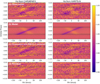 |
Fig. 2 Transmission spectral matrices for the Hα line from the CARMENES observations (left) and the HARPS-N observations (right). The colour bar indicates the value of relative flux. (a) The observed transmission spectra. The x-axis is wavelength expressed in RV relative to the Hα line centre (6562.79 Å) in the stellar rest frame. The horizontal dashed lines indicate the four contacts of transit. (b) The best-fit model from the MCMC analysis. The model includes the Hα transmission spectrum and the stellar line profile change (i.e. the CLV and RM effects). The blue dashed line indicates the RV of the planetary orbital motion plus a constant shift (Vcentre). Although the models extend into the ingress and egress regions on the matrices, the fit was only performed on the fully in-transit data. (c) The observed transmission spectra with the RM and CLV effects corrected. (d) The residual between the observation and the model. |
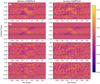 |
Fig. 3 Same as Fig. 2 but for the Hβ line (left) and the Hγ line (right) from the HARPS-N observations. |
3.2 Hβ and Hγ transmission spectrum
The Hβ and Hγ lines are only covered by the HARPS-N spectrograph. The absorption signals are relatively weak compared to the Hα line. The best-fit parameters are shown in Table 2 with the final transmission spectra in Fig. 8. The detection of Hβ is clear while the Hγ signal is less prominent. The line depth of the Hβ absorption is smaller than that of the Hα line, but their FWHM values are relatively similar to each other. This is also the case for the Hα and Hβ lines in KELT-9b(Cauley et al. 2019; Wyttenbach et al. 2020) and KELT-20b (Casasayas-Barris et al. 2019).
Fit results of the transmission spectral matrices.
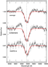 |
Fig. 4 Transmission spectra of the Hα line. The black circles represent spectra binned every five points (~0.15 Å) and the grey lines represent the original spectra (i.e. ~0.03 Å per point). The red lines indicate the best-fit Gaussian functions. The vertical dashed line indicates the rest wavelength line centre. The CLV and RM effects are corrected. An offset of the y-axis is applied to the spectra for clarity. |
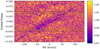 |
Fig. 5 Combined transmission spectral matrix of the CARMENES and HARPS-N results for the Hα line. The stellar line profile change due to the CLV and RM effects has been removed before averaging. The horizontal dashed linesindicate the four contacts of transit and the diagonal dashed lines denote the planetary orbital RV. |
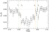 |
Fig. 6 Time series of the Hα equivalent width. The values are measured on the combined transmission spectral matrix in Fig. 5. The vertical dashed lines indicate the first (T1), second (T2), third (T3), and fourth (T4) contacts of the transit. The horizontal line denotes WHα = 0. |
3.3 Model of the balmer lines
3.3.1 Estimation of the atmospheric conditions
To obtain a rough estimate of the possible atmospheric conditions, and before modelling the lines, we can use the Lecavelier Des Etangs et al. (2008) formula to estimate the atmospheric scale height in the region probed by the Balmer lines. Indeed, the altitude of absorption z is proportional to the hydrogen Balmer line oscillator strengths ln(gf): Δz = HΔln(gf), where H = kBT∕μg is the pressure scale height.The ln(gf) values are 1.635, −0.046, and −1.029 for the Hα, Hβ, and Hγ lines, respectively. Taking into account all our measurements from CARMENES and HARPS-N, we computed H = 9200 ± 1200 km. Considering the decrease in the gravity g with altitude, we estimated that T∕μ ≃ 15 100 ± 2100 [K/u] (at z ~ 1.2RP). As it is likely that molecular hydrogen is dissociated under these conditions and the atmosphere is dominated by a mixture of ionised and neutral hydrogen and helium, we can further assume that μ is between 0.66 and 1.26. Hence, we estimated the upper atmosphere temperature to be between 8600 and 21 700 K. The lower end of the T range should be preferred since when the temperature increases, the amount of ionised hydrogen increases, making μ decreases as well.
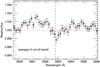 |
Fig. 7 Average out-of-transit spectrum of the Hα transmission spectral matrix in Fig. 5. The vertical dashed line denotes the line centre. These spectral features likely originate from the stellar pulsation. |
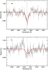 |
Fig. 8 Transmission spectra of the Hβ line (upper panel) and the Hγ line (lower panel). |
3.3.2 Model set-up
To interpret the observed Balmer lines in WASP-33b, we employed the PArker Winds and Saha-BoltzmanN (PAWN) atmospheric model developed by Wyttenbach et al. (2020). This tool is a one-dimensional model of an exoplanet upper atmosphere linked to an MCMC retrieval algorithm. Its purpose is to retrieve parameters of the thermosphere regions (e.g. the temperature and mass-loss rate) from high-resolution transmission spectra. Key features of the PAWN model are summarised below. First, we can choose the atmospheric structure to be hydrostatic (barometric law) or hydrodynamic (Parker wind transonic solution), with the base density or the mass-loss rate being a free parameter, respectively. The atmospheric profile is assumed to be isothermal in both cases, with the temperature being an additional free parameter. We also assume the atmosphere to be in chemical equilibrium, with solar abundances. We use a chemical grid calculated with the equilibrium chemistry code presented in Mollière et al. (2017), from which we interpolate the volume mixing ratios and other useful quantities according to the atmospheric structure. As we detected Balmer lines, we focussed on the neutral hydrogen. In local thermodynamic equilibrium (LTE), the number densities of the different electronic states follow the Boltzmann distribution. Then, the opacities have a Voigt profile and follow the prescriptions of Kurucz (1979, 1992) and Sharp & Burrows (2007). Finally, the transmission spectrum is computed following Mollière et al. (2019). The line profiles are broadened taking into account the planetary rotation (tidally locked solid body rotation perpendicular to the orbital plane). The model is also convolved, binned, and normalised in order to be comparable to the data.
On top of the atmospheric model parameters presented above, each line centre is a free parameter. For other planetary parameters (e.g. mass and radius), we used the same values as presented in Table 2 of Yan et al. (2019). For every MCMC chain, we used ten walkers for each parameter during 2500 steps, with a burn-in size of 500 steps. For each parameter, we used a uniform or log-uniform prior. For the mass-loss rate we put a lower boundary for the prior at log10(Ṁ [g s−1]) = 9, as it is expected that WASP-33b is undergoing strong atmospheric escape (Fossati et al. 2018). We tried to fit hydrostatic and hydrodynamic structures to see if one structure would be preferred. The Bayesian information criterion (BIC) allowed us to compare theresults of different models, and to choose the best-fitting model.
3.3.3 Model results
We performed MCMC chains on each individual Balmer absorption line from HARPS-N and CARMENES. We also fitted the three Balmer linessimultaneously, using the combined HARPS-N and CARMENES result. It is important to note that since the depth of the Hα line is not the same for the two instruments, we would expect some differences in the retrieved parameters.
The results from the MCMC model fitting are summarised in Table 3 for the case of a hydrodynamic atmosphere in LTE. For each detection, the retrieved parameters are compatible. The combined fit (all Balmer lines from HARPS-N and CARMENES) points towards a thermospheric temperature of  K and a mass-loss rate of
  g s−1. The best-fit spectra and the correlation diagram of the combined fit are presented in Figs. 9 and 10, respectively. Before interpreting this result, we mention that for each scenario (line or instrument), the absorption line was fitted equally well by a hydrostatic structure (ΔBIC < 1). This is because, for a hot Jupiter, it is often possible to find a very similar atmospheric structure for both cases, especially when the temperature is high (Wyttenbach et al. 2020). Nevertheless, an evaporating scenario could be preferred for WASP-33b, as suggested by forward modelling (Fossati et al. 2018). This latter study predicted a mass-loss rate of about 1011 g s−1 for WASP-33b, which is well in line with our retrieved mass-loss rate.
Our retrieved mass-loss rate of  g s−1 is close to the maximum energy-limited mass-loss rate (Fossati et al. 2018). This could suggest that the heating efficiency is high (of the order of 10–100%), meaning that most of the irradiation energy goes into expansion (PdV work) and escape. However, according to Salz et al. (2016), when a hot Jupiter has a relatively high gravitational potential (such as WASP-33b), the heating efficiency should decrease by several orders of magnitude. This hints that the energy-limited computation of Fossati et al. (2018) may not be complete and that some energy sources are not taken into consideration. Indeed, García Muñoz & Schneider (2019) suggested that hot Jupiters orbiting early-type stars could undergo a Balmer-driven evaporation. This mechanism has been proposed for the UHJ KELT-9b and is supportedby the observations of the Balmer series in its thermosphere (Yan & Henning 2018; Wyttenbach et al. 2020). This Balmer-driven mechanism takes place when a sufficient quantity of excited hydrogen is present in the thermosphere and the planet is irradiated with intense stellar near-ultraviolet radiation. In that case, the energy absorbed in the thermosphere from the stellar Balmer irradiation exceeds that absorbed from the stellar high-energy EUV irradiation. Thus, the thermosphere undergoes a stronger heating and expansion, leading to a higher mass-loss rate, even if the heating efficiency stays moderate. The measured mass-loss rate for WASP-33b is
  g s−1, while that of KELT-9b is Ṁ = 1012.8 ± 0.3 g s−1 (Wyttenbach et al. 2020). These measurements are compatible with a Balmer-driven evaporation, since WASP-33b orbits an A5 star, while KELT-9b orbits an A0V star, where the Balmer flux is extremely high.
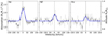 |
Fig. 9 Best-fit PAWN models (blue lines) and the observed transmission spectra (grey lines and black points) in the planetary rest frame. The PAWN models are shown for the case of a hydrodynamically expanding atmosphere in LTE. |
MCMC results of the PAWN modeling for an atmosphere in hydrodynamic expansion and in LTE.
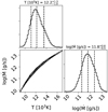 |
Fig. 10 Correlation diagram of the MCMC posterior distributions in the case of a hydrodynamic atmosphere in LTE. The result is for the combined fit of all Balmer lines from HARPS-N and CARMENES. The retrieved parameters are the thermospheric temperature ( |
4 Conclusions
We observed four transits of the UHJ WASP-33b with the CARMENES and HARPS-N spectrographs. After the correction of the RM and CLV effects, we detected the Balmer Hα, Hβ, and Hγ transmission spectra of the planetary atmosphere. The combined Hα transmission spectrum has a large absorption depth of 0.99 ± 0.05%, indicating that the line probes neutral hydrogen atoms in the high-altitude thermosphere. Although the detection of the Balmer lines is unambiguous, the strengths of the lines are affected by the stellar pulsation. Future modelling and correction of the spectral pulsation feature will enable us to better constrain the line strength.
We fitted the observed Balmer lines using the PAWN model assuming that the atmosphere is hydrodynamic and in LTE. The model fit returns a thermospheric temperature of  K and a mass-loss rate
  g s−1. The high mass-loss rate is consistent with theoretical predictions for UHJs orbiting early-type stars (e.g. Fossati et al. 2018; García Muñoz & Schneider 2019).
Balmer lines have so far been detected in five UHJs (KELT-9b, KELT-20b/MASCARA-2b, WASP-12b, WASP-121b, and WASP-33b). Balmer absorption is probably a common spectral feature in the transmission spectra of UHJs because their hot atmospheres are intensively irradiated by their host stars, which could produce a large number of hydrogen atoms in the excited state. However, for some UHJs, their low atmospheric scale heights (see e.g. the case of WASP-189b, Cauley et al. 2020b) or the RM effect (e.g. Casasayas-Barris et al. 2020) could hamper the detection of the Balmer features. Extending the observations to a larger UHJ sample will enable a systematic study of Balmer lines and thermospheric conditions.
Acknowledgements
We thank the referee for the useful comments. F.Y. acknowledges the support of the DFG priority program SPP 1992 “Exploring the Diversity of Extrasolar Planets (RE 1664/16-1)”. CARMENES is an instrument for the Centro Astronómico Hispano-Alemán (CAHA) at Calar Alto (Almería, Spain), operated jointly by the Junta de Andalucía and the Instituto de Astrofísica de Andalucía (CSIC). CARMENES was funded by the Max-Planck-Gesellschaft (MPG), the Consejo Superior de Investigaciones Científicas (CSIC), the Ministerio de Economía y Competitividad (MINECO) and the European Regional Development Fund (ERDF) through projects FICTS-2011-02, ICTS-2017-07-CAHA-4, and CAHA16-CE-3978, and the members of the CARMENES Consortium (Max-Planck-Institut für Astronomie, Instituto de Astrofísica de Andalucía, Landessternwarte Königstuhl, Institut de Ciències de l’Espai, Institut für Astrophysik Göttingen, Universidad Complutense de Madrid, Thüringer Landessternwarte Tautenburg, Instituto de Astrofísica de Canarias, Hamburger Sternwarte, Centro de Astrobiología and Centro Astronómico Hispano-Alemán), with additional contributions by the MINECO, the Deutsche Forschungsgemeinschaft through the Major Research Instrumentation Programme and Research Unit FOR2544 “Blue Planets around Red Stars”, the Klaus Tschira Stiftung, the states of Baden-Württemberg and Niedersachsen, and by the Junta de Andalucía. Based on data from the CARMENES data archive at CAB (CSIC-INTA). We acknowledge financial support from the Agencia Estatal de Investigación of the Ministerio de Ciencia, Innovación y Universidades and the ERDF through projects PID2019-109522GB-C51/2/3/4, PGC2018-098153-B-C33, AYA2016-79425-C3-1/2/3-P, ESP2016-80435-C2-1-R and the Centre of Excellence “Severo Ochoa” and “María de Maeztu” awards to the Instituto de Astrofísica de Canarias (SEV-2015-0548), Instituto de Astrofísica de Andalucía (SEV-2017-0709), and Centro de Astrobiología (MDM-2017-0737), and the Generalitat de Catalunya/CERCA programme. A.W. acknowledges the financial support of the SNSF by grant number P400P2_186765. P.M. acknowledges support from the European Research Council under the Horizon 2020 Framework Program via ERC grant 832428. I.S. acknowledges funding from the European Research Council (ERC) under the European Union’s Horizon 2020 research and innovation program under grant agreement No 694513. M.L. achkowledges the funding from the project ESP2017-87143-R. This work is based on observations made with the Italian Telescopio Nazionale Galileo (TNG) operated on the island of La Palma by the Fundación Galileo Galilei of the INAF (Istituto Nazionale di Astrofisica) at the Spanish Observatorio del Roque de los Muchachos of the Instituto de Astrofisica de Canarias.
Appendix A Additional figure
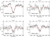 |
Fig. A.1 Hα transmission spectra of the four nights. The grey lines indicate the original spectra and the black points indicate spectra binned every five points. The red lines show the same best-fit Gaussian functions as in Fig. 4. |
References
- Allart, R., Bourrier, V., Lovis, C., et al. 2018, Science, 362, 1384 [Google Scholar]
- Arcangeli, J., Désert, J.-M., Line, M. R., et al. 2018, ApJ, 855, L30 [NASA ADS] [CrossRef] [Google Scholar]
- Barnes, J. R., Haswell, C. A., Staab, D., & Anglada-Escudé, G. 2016, MNRAS, 462, 1012 [Google Scholar]
- Bell, T. J., & Cowan, N. B. 2018, ApJ, 857, L20 [NASA ADS] [CrossRef] [Google Scholar]
- Ben-Yami, M., Madhusudhan, N., Cabot, S. H. C., et al. 2020, ApJ, 897, L5 [CrossRef] [Google Scholar]
- Bourrier, V., Kitzmann, D., Kuntzer, T., et al. 2020a, A&A, 637, A36 [CrossRef] [EDP Sciences] [Google Scholar]
- Bourrier, V., Ehrenreich, D., Lendl, M., et al. 2020b, A&A, 635, A205 [NASA ADS] [CrossRef] [EDP Sciences] [Google Scholar]
- Brogi, M., de Kok, R. J., Albrecht, S., et al. 2016, ApJ, 817, 106 [Google Scholar]
- Cabot, S. H. C., Madhusudhan, N., Welbanks, L., Piette, A., & Gandhi, S. 2020, MNRAS, 494, 363 [NASA ADS] [CrossRef] [Google Scholar]
- Casasayas-Barris, N., Pallé, E., Yan, F., et al. 2018, A&A, 616, A151 [NASA ADS] [CrossRef] [EDP Sciences] [Google Scholar]
- Casasayas-Barris, N., Pallé, E., Yan, F., et al. 2019, A&A, 628, A9 [NASA ADS] [CrossRef] [EDP Sciences] [Google Scholar]
- Casasayas-Barris, N., Pallé, E., Yan, F., et al. 2020, A&A, 635, A206 [NASA ADS] [CrossRef] [EDP Sciences] [Google Scholar]
- Cauley, P. W., Redfield, S., Jensen, A. G., & Barman, T. 2016, AJ, 152, 20 [NASA ADS] [CrossRef] [Google Scholar]
- Cauley, P. W., Redfield, S., & Jensen, A. G. 2017a, AJ, 153, 217 [NASA ADS] [CrossRef] [Google Scholar]
- Cauley, P. W., Redfield, S., & Jensen, A. G. 2017b, AJ, 153, 185 [NASA ADS] [CrossRef] [Google Scholar]
- Cauley, P. W., Shkolnik, E. L., Ilyin, I., et al. 2019, AJ, 157, 69 [NASA ADS] [CrossRef] [Google Scholar]
- Cauley, P. W., Wang, J., Shkolnik, E. L., et al. 2020a, AAS J., submitted [arXiv:2010.02118] [Google Scholar]
- Cauley, P. W., Shkolnik, E. L., Ilyin, I., et al. 2020b, Research Notes AAS, 4, 53 [CrossRef] [Google Scholar]
- Chen, G., Casasayas-Barris, N., Pallé, E., et al. 2020, A&A, 635, A171 [CrossRef] [Google Scholar]
- Christie, D., Arras, P., & Li, Z.-Y. 2013, ApJ, 772, 144 [NASA ADS] [CrossRef] [Google Scholar]
- Collier Cameron, A., Guenther, E., Smalley, B., et al. 2010, MNRAS, 407, 507 [NASA ADS] [CrossRef] [Google Scholar]
- Cubillos, P. E., Fossati, L., Koskinen, T., et al. 2020, AJ, 159, 111 [Google Scholar]
- Czesla, S., Klocová, T., Khalafinejad, S., Wolter, U., & Schmitt, J. H. M. M. 2015, A&A, 582, A51 [NASA ADS] [CrossRef] [EDP Sciences] [Google Scholar]
- Daylan, T., Günther, M. N., Mikal-Evans, T., et al. 2019, ArXiv e-prints [arXiv:1909.03000] [Google Scholar]
- Ehrenreich, D., Bourrier, V., Wheatley, P. J., et al. 2015, Nature, 522, 459 [Google Scholar]
- Ehrenreich, D., Lovis, C., Allart, R., et al. 2020, Nature, 580, 597 [Google Scholar]
- Foreman-Mackey, D., Hogg, D. W., Lang, D., & Goodman, J. 2013, PASP, 125, 306 [Google Scholar]
- Fossati, L., Haswell, C. A., Froning, C. S., et al. 2010, ApJ, 714, L222 [Google Scholar]
- Fossati, L., Koskinen, T., Lothringer, J. D., et al. 2018, ApJ, 868, L30 [NASA ADS] [CrossRef] [Google Scholar]
- García Muñoz, A., & Schneider, P. C. 2019, ApJ, 884, L43 [CrossRef] [Google Scholar]
- Gibson, N. P., Merritt, S., Nugroho, S. K., et al. 2020, MNRAS, 493, 2215 [Google Scholar]
- Haynes, K., Mandell, A. M., Madhusudhan, N., Deming, D., & Knutson, H. 2015, ApJ, 806, 146 [NASA ADS] [CrossRef] [Google Scholar]
- Helling, C., Gourbin, P., Woitke, P., & Parmentier, V. 2019, A&A, 626, A133 [CrossRef] [Google Scholar]
- Hoeijmakers, H. J., Ehrenreich, D., Heng, K., et al. 2018, Nature, 560, 453 [NASA ADS] [CrossRef] [Google Scholar]
- Hoeijmakers, H. J., Ehrenreich, D., Kitzmann, D., et al. 2019, A&A, 627, A165 [NASA ADS] [CrossRef] [EDP Sciences] [Google Scholar]
- Hoeijmakers, H. J., Cabot, S. H. C., Zhao, L., et al. 2020, A&A, 641, A120 [EDP Sciences] [Google Scholar]
- Huang, C., Arras, P., Christie, D., & Li, Z.-Y. 2017, ApJ, 851, 150 [NASA ADS] [CrossRef] [Google Scholar]
- Iorio, L. 2016, MNRAS, 455, 207 [NASA ADS] [CrossRef] [Google Scholar]
- Jensen, A. G., Redfield, S., Endl, M., et al. 2012, ApJ, 751, 86 [Google Scholar]
- Jensen, A. G., Cauley, P. W., Redfield, S., Cochran, W. D., & Endl, M. 2018, AJ, 156, 154 [NASA ADS] [CrossRef] [Google Scholar]
- Johnson, M. C., Cochran, W. D., Collier Cameron, A., & Bayliss, D. 2015, ApJ, 810, L23 [NASA ADS] [CrossRef] [Google Scholar]
- Kesseli, A. Y., Snellen, I. A. G., Alonso-Floriano, F. J., Mollière, P., & Serindag, D. B. 2020, AJ, 160, 228 [CrossRef] [Google Scholar]
- Kitzmann, D., Heng, K., Rimmer, P. B., et al. 2018, ApJ, 863, 183 [Google Scholar]
- Komacek, T. D., & Tan, X. 2018, Research Notes AAS, 2, 36 [NASA ADS] [CrossRef] [Google Scholar]
- Kovács, G., Kovács, T., Hartman, J. D., et al. 2013, A&A, 553, A44 [NASA ADS] [CrossRef] [EDP Sciences] [Google Scholar]
- Kreidberg, L., Line, M. R., Parmentier, V., et al. 2018, AJ, 156, 17 [NASA ADS] [CrossRef] [Google Scholar]
- Kurucz, R. L. 1979, ApJS, 40, 1 [NASA ADS] [CrossRef] [Google Scholar]
- Kurucz, R. L. 1992, IAU Symp., 149, 225 [Google Scholar]
- Lampón, M., López-Puertas, M., Lara, L. M., et al. 2020, A&A, 636, A13 [CrossRef] [EDP Sciences] [Google Scholar]
- Lecavelier Des Etangs, A., Pont, F., Vidal-Madjar, A., & Sing, D. 2008, A&A, 481, L83 [NASA ADS] [CrossRef] [Google Scholar]
- Lecavelier des Etangs, A., Bourrier, V., Wheatley, P. J., et al. 2012, A&A, 543, L4 [NASA ADS] [CrossRef] [EDP Sciences] [Google Scholar]
- Lehmann, H., Guenther, E., Sebastian, D., et al. 2015, A&A, 578, L4 [NASA ADS] [CrossRef] [EDP Sciences] [Google Scholar]
- Lothringer, J. D., Barman, T., & Koskinen, T. 2018, ApJ, 866, 27 [NASA ADS] [CrossRef] [Google Scholar]
- Louden, T., & Wheatley, P. J. 2015, ApJ, 814, L24 [NASA ADS] [CrossRef] [Google Scholar]
- Mansfield, M., Bean, J. L., Line, M. R., et al. 2018, AJ, 156, 10 [NASA ADS] [CrossRef] [Google Scholar]
- Mansfield, M., Bean, J. L., Stevenson, K. B., et al. 2020, ApJ, 888, L15 [NASA ADS] [CrossRef] [Google Scholar]
- Mollière, P., van Boekel, R., Bouwman, J., et al. 2017, A&A, 600, A10 [NASA ADS] [CrossRef] [EDP Sciences] [Google Scholar]
- Mollière, P., Wardenier, J. P., van Boekel, R., et al. 2019, A&A, 627, A67 [NASA ADS] [CrossRef] [EDP Sciences] [Google Scholar]
- Nortmann, L., Pallé, E., Salz, M., et al. 2018, Science, 362, 1388 [Google Scholar]
- Nugroho, S. K., Kawahara, H., Masuda, K., et al. 2017, AJ, 154, 221 [NASA ADS] [CrossRef] [Google Scholar]
- Nugroho, S. K., Gibson, N. P., de Mooij, E. J. W., et al. 2020a, ApJ, 898, L31 [CrossRef] [Google Scholar]
- Nugroho, S. K., Gibson, N. P., de Mooij, E. J. W., et al. 2020b, MNRAS, 496, 504 [CrossRef] [Google Scholar]
- Owen, J. E. 2019, Annu. Rev. Earth Planet. Sci., 47, 67 [CrossRef] [Google Scholar]
- Palle, E., Nortmann, L., Casasayas-Barris, N., et al. 2020, A&A, 638, A61 [EDP Sciences] [Google Scholar]
- Parmentier, V., Line, M. R., Bean, J. L., et al. 2018, A&A, 617, A110 [NASA ADS] [CrossRef] [EDP Sciences] [Google Scholar]
- Pino, L., Désert, J.-M., Brogi, M., et al. 2020, ApJ, 894, L27 [Google Scholar]
- Queloz, D., Eggenberger, A., Mayor, M., et al. 2000, A&A, 359, L13 [NASA ADS] [Google Scholar]
- Quirrenbach, A., Amado, P. J., Ribas, I., et al. 2018, Proc. SPIE Conf. Ser., 10702, 107020W [Google Scholar]
- Salz, M., Czesla, S., Schneider, P. C., & Schmitt, J. H. M. M. 2016, A&A, 586, A75 [NASA ADS] [CrossRef] [EDP Sciences] [Google Scholar]
- Salz, M., Czesla, S., Schneider, P. C., et al. 2018, A&A, 620, A97 [NASA ADS] [CrossRef] [EDP Sciences] [Google Scholar]
- Sharp, C. M., & Burrows, A. 2007, ApJS, 168, 140 [NASA ADS] [CrossRef] [Google Scholar]
- Sing, D. K., Lavvas, P., Ballester, G. E., et al. 2019, AJ, 158, 91 [Google Scholar]
- Snellen, I. A. G., de Kok, R. J., de Mooij, E. J. W., & Albrecht, S. 2010, Nature, 465, 1049 [NASA ADS] [CrossRef] [PubMed] [Google Scholar]
- Spake, J. J., Sing, D. K., Evans, T. M., et al. 2018, Nature, 557, 68 [Google Scholar]
- Stangret, M., Casasayas-Barris, N., Pallé, E., et al. 2020, A&A, 638, A26 [CrossRef] [EDP Sciences] [Google Scholar]
- Stevenson, K. B., Bean, J. L., Madhusudhan, N., & Harrington, J. 2014, ApJ, 791, 36 [NASA ADS] [CrossRef] [Google Scholar]
- Tian, F., Toon, O. B., Pavlov, A. A., & De Sterck H. 2005, ApJ, 621, 1049 [NASA ADS] [CrossRef] [Google Scholar]
- Turner, J. D., de Mooij, E. J. W., Jayawardhana, R., et al. 2020, ApJ, 888, L13 [NASA ADS] [CrossRef] [Google Scholar]
- Valyavin, G. G., Gadelshin, D. R., Valeev, A. F., et al. 2018, Astrophys. Bull., 73, 225 [CrossRef] [Google Scholar]
- Vidal-Madjar, A., Lecavelier des Etangs, A., Désert, J.-M., et al. 2003, Nature, 422, 143 [Google Scholar]
- von Essen, C., Czesla, S., Wolter, U., et al. 2014, A&A, 561, A48 [NASA ADS] [CrossRef] [EDP Sciences] [Google Scholar]
- von Essen, C., Mallonn, M., Welbanks, L., et al. 2019, A&A, 622, A71 [NASA ADS] [CrossRef] [EDP Sciences] [Google Scholar]
- von Essen, C., Mallonn, M., Borre, C. C., et al. 2020, A&A, 639, A34 [CrossRef] [EDP Sciences] [Google Scholar]
- Watanabe, N., Narita, N., & Johnson, M. C. 2020, PASJ, 72, 19 [CrossRef] [Google Scholar]
- Wong, I., Shporer, A., Kitzmann, D., et al. 2020, AJ, 160, 88 [CrossRef] [Google Scholar]
- Wyttenbach, A., Ehrenreich, D., Lovis, C., Udry, S., & Pepe, F. 2015, A&A, 577, A62 [NASA ADS] [CrossRef] [EDP Sciences] [Google Scholar]
- Wyttenbach, A., Mollière, P., Ehrenreich, D., et al. 2020, A&A, 638, A87 [EDP Sciences] [Google Scholar]
- Yan, F., & Henning, T. 2018, Nat. Astron., 2, 714 [NASA ADS] [CrossRef] [Google Scholar]
- Yan, F., Fosbury, R. A. E., Petr-Gotzens, M. G., et al. 2015a, Int. J. Astrobiol., 14, 255 [CrossRef] [Google Scholar]
- Yan, F., Fosbury, R. A. E., Petr-Gotzens, M. G., Zhao, G., & Pallé, E. 2015b, A&A, 574, A94 [NASA ADS] [CrossRef] [EDP Sciences] [Google Scholar]
- Yan, F., Pallé, E., Fosbury, R. A. E., Petr-Gotzens, M. G., & Henning, T. 2017, A&A, 603, A73 [NASA ADS] [CrossRef] [EDP Sciences] [Google Scholar]
- Yan, F., Casasayas-Barris, N., Molaverdikhani, K., et al. 2019, A&A, 632, A69 [NASA ADS] [CrossRef] [EDP Sciences] [Google Scholar]
- Yan, F., Pallé, E., Reiners, A., et al. 2020, A&A, 640, L5 [CrossRef] [EDP Sciences] [Google Scholar]
- Yelle, R. V. 2004, Icarus, 170, 167 [NASA ADS] [CrossRef] [Google Scholar]
- Zhang, M., Knutson, H. A., Kataria, T., et al. 2018, AJ, 155, 83 [NASA ADS] [CrossRef] [Google Scholar]
All Tables
MCMC results of the PAWN modeling for an atmosphere in hydrodynamic expansion and in LTE.
All Figures
|
Fig. 1 Signal-to-noise ratio per wavelength point (~0.03 Å) at the Hα line centre. The dashed lines indicate the beginning and end of transit. |
| In the text | |
|
Fig. 2 Transmission spectral matrices for the Hα line from the CARMENES observations (left) and the HARPS-N observations (right). The colour bar indicates the value of relative flux. (a) The observed transmission spectra. The x-axis is wavelength expressed in RV relative to the Hα line centre (6562.79 Å) in the stellar rest frame. The horizontal dashed lines indicate the four contacts of transit. (b) The best-fit model from the MCMC analysis. The model includes the Hα transmission spectrum and the stellar line profile change (i.e. the CLV and RM effects). The blue dashed line indicates the RV of the planetary orbital motion plus a constant shift (Vcentre). Although the models extend into the ingress and egress regions on the matrices, the fit was only performed on the fully in-transit data. (c) The observed transmission spectra with the RM and CLV effects corrected. (d) The residual between the observation and the model. |
| In the text | |
|
Fig. 3 Same as Fig. 2 but for the Hβ line (left) and the Hγ line (right) from the HARPS-N observations. |
| In the text | |
|
Fig. 4 Transmission spectra of the Hα line. The black circles represent spectra binned every five points (~0.15 Å) and the grey lines represent the original spectra (i.e. ~0.03 Å per point). The red lines indicate the best-fit Gaussian functions. The vertical dashed line indicates the rest wavelength line centre. The CLV and RM effects are corrected. An offset of the y-axis is applied to the spectra for clarity. |
| In the text | |
|
Fig. 5 Combined transmission spectral matrix of the CARMENES and HARPS-N results for the Hα line. The stellar line profile change due to the CLV and RM effects has been removed before averaging. The horizontal dashed linesindicate the four contacts of transit and the diagonal dashed lines denote the planetary orbital RV. |
| In the text | |
|
Fig. 6 Time series of the Hα equivalent width. The values are measured on the combined transmission spectral matrix in Fig. 5. The vertical dashed lines indicate the first (T1), second (T2), third (T3), and fourth (T4) contacts of the transit. The horizontal line denotes WHα = 0. |
| In the text | |
|
Fig. 7 Average out-of-transit spectrum of the Hα transmission spectral matrix in Fig. 5. The vertical dashed line denotes the line centre. These spectral features likely originate from the stellar pulsation. |
| In the text | |
|
Fig. 8 Transmission spectra of the Hβ line (upper panel) and the Hγ line (lower panel). |
| In the text | |
|
Fig. 9 Best-fit PAWN models (blue lines) and the observed transmission spectra (grey lines and black points) in the planetary rest frame. The PAWN models are shown for the case of a hydrodynamically expanding atmosphere in LTE. |
| In the text | |
|
Fig. 10 Correlation diagram of the MCMC posterior distributions in the case of a hydrodynamic atmosphere in LTE. The result is for the combined fit of all Balmer lines from HARPS-N and CARMENES. The retrieved parameters are the thermospheric temperature ( |
| In the text | |
|
Fig. A.1 Hα transmission spectra of the four nights. The grey lines indicate the original spectra and the black points indicate spectra binned every five points. The red lines show the same best-fit Gaussian functions as in Fig. 4. |
| In the text | |
Current usage metrics show cumulative count of Article Views (full-text article views including HTML views, PDF and ePub downloads, according to the available data) and Abstracts Views on Vision4Press platform.
Data correspond to usage on the plateform after 2015. The current usage metrics is available 48-96 hours after online publication and is updated daily on week days.
Initial download of the metrics may take a while.