| Issue |
A&A
Volume 645, January 2021
|
|
|---|---|---|
| Article Number | A98 | |
| Number of page(s) | 13 | |
| Section | Interstellar and circumstellar matter | |
| DOI | https://doi.org/10.1051/0004-6361/202037773 | |
| Published online | 20 January 2021 | |
The hot interstellar medium towards 4U 1820-30: a Bayesian analysis
1
SRON Netherlands Institute for Space Research,
Sorbonnelaan 2,
3584 CA Utrecht,
The Netherlands
e-mail: This email address is being protected from spambots. You need JavaScript enabled to view it.
2
Anton Pannekoek Astronomical Institute, University of Amsterdam,
PO Box 94249,
1090 GE Amsterdam,
The Netherlands
3
Combient Mix AB,
Box 2150,
40313 Göteborg,
Sweden
Received:
19
February
2020
Accepted:
2
December
2020
Abstract
Context. High-ionisation lines in the soft X-ray band are generally associated to either interstellar hot gas along the line of sight or to photoionised gas intrinsic to the source. In the low-mass X-ray binary 4U 1820-30, the nature of these lines is not well understood.
Aims. We aim to characterise the ionised gas present along the line of sight towards 4U 1820-30 producing the X-ray absorption lines of Mg XI, Ne IX, Fe XVII, O VII, and O VIII.
Methods. We analysed all the observations available for this source in the XMM-Newton and Chandra archives that were taken with the RGS, HETG, and LETG spectrometers. We accurately examined the high-resolution grating spectra using a standard X-ray analysis procedure based on the C-statistic and using Bayesian parameter inference. We tested two physical models which describe a plasma in either collisional ionisation or photoionisation equilibrium. We adopted the Bayesian model comparison to statistically compare the different combinations of models used for the analysis.
Results. We find that the lines are consistent with hot gas in the interstellar medium rather than the intrinsic gas of the X-ray binary. Our best-fit model reveals the presence of a collisionally ionised plasma with a temperature of T = (1.98 ± 0.05) × 106 K. The photoionisation model fails to fit the Fe XVII line (which is detected with a significance of 6.5σ) because of the low column density predicted by the model. Moreover, the low inclination of the binary system is likely the reason for the non-detection of ionised gas intrinsic to the source.
Key words: X-rays: binaries / X-rays: individuals: 4U 1820-30 / X-rays: ISM / ISM: lines and bands
© ESO 2021
1 Introduction
In the space among the stars resides interstellar matter, a vast and heterogeneous mixture of atoms, molecules, and solid dust grains. As a function of the temperature and density of the diffuse gas, the interstellar medium (ISM) can be classified in three main phases (Ferrière 2001, and reference therein): a cold phase (with temperature TISM < 100 K and density nH = 10−106 cm−3), a warm phase (TISM ~ 8000 K and nH = 0.2−0.5 cm−3, including both warm neutral and warm photoionised gases), and a hot phase (TISM ~ 106 K and nH ~ 6.5 × 10⁻³ cm−3).
The hot ISM (also known as hot coronal gas) in the Milky Way was discovered through the detection of the soft X-ray background in the 0.1–1 keV energy range (Tanaka & Bleeker 1977) and through the UV O VI absorption lines in the spectra of OB stars (Jenkins 1978). It has been proposed that the hot phase could account for much of the missing baryons within the Galactic halo, and could be used as a tracer of energetic feedback from stars and supernovae, which plays an important role in shaping the ecosystem of the Galaxy (McKee & Ostriker 1977; Miller & Bregman 2013).
In the past several years it has been demonstrated that the hot phase of the ISM can be successfully characterised through X-ray absorption line spectroscopy (e.g. Futamoto et al. 2004; Yao & Wang 2005; Wang 2010; Liao et al. 2013; Gatuzz & Churazov 2018). Through the measurements of absorption lines produced by various ions in the spectra of bright X-ray sources, primarily active galactic nuclei and X-ray binaries, it is possible to set physical constraints on the ionisation process, temperature, kinematics, and chemical abundances of the hot gas. It is also possible to study its distribution in both the disc and the halo of the Galaxy.
However, the interpretation of these high-ionisation absorption lines can be uncertain. Indeed, these features are not always clearly associated with the interstellar hot gas in a collisional ionisation equilibrium state. In some systems, they can be produced by an absorber intrinsic to the background X-ray source and photoionised by its strong radiation. The presence of multiple blueshifted and/or variable high-ionisation lines indicates a wind outflowing in our line of sight, in particular from the accretion disc of stellar-mass black holes (e.g. Lee et al. 2002; Parmar et al. 2002; Ueda et al. 2004; Díaz Trigo et al. 2006). On the other hand, in dipping X-ray binaries, strong absorption lines that are local to the source are found not to be blueshifted and these are thought to be associated with the corona of the accretion disc (Sidoli et al. 2001a; Díaz Trigo et al. 2006). Therefore, for some sources, it might be difficult to discern whether or not the presence of high-ionisation lines in the spectrum is associated with a collisionally ionised gas in interstellar space rather than with a photoionised absorber associated to the X-ray source. One example is the source that we analyse in the present work.
4U 1820-30 is a well-known bright X-ray source in the Sagitarius constellation first observed by the Uhuru satellite (Giacconi et al. 1972). This source is an accreting neutron star low-mass X-ray binary residing in the globular cluster NGC 6624 at (l, b) = (2. °8,−7. °9). The binary consists in an ultracompact system with an orbital period of ~ 11 min and a size of r = 1.3 × 1010 cm (Stella et al. 1987). The companion has been identified as a He-white dwarf. The distance of 4U 1820-30 was determined to be 7.6 ±0.4 kpc (Kuulkers et al. 2003), and is therefore very close to the Galactic centre. Consequently, our line of sight samples the entire inner Galactic disc radially to a height of ~1 kpc from the Galactic plane.
The soft X-ray band of 4U 1820-30 was demonstrated to be a useful tool with which to study the different phases of the ISM simultaneously. In previous works, the cold phase was studied through the oxygen, neon, and iron photoelectric edges detected in high-resolution X-ray spectra (Juett et al. 2004, 2006; Miller et al. 2009). An accurate analysis of the oxygen K-edge and iron L-edges was performed by Costantini et al. (2012; hereafter C12) wherein these authors modelled the absorption by both cold gas and interstellar dust. The detection of low-ionisation lines1 such as Ne II (14.608 Å), Ne III (14.508 Å), O II (23.351 Å), and O III (23.028 Å) indicates the presence of a slightly ionised gas towards 4U 1820-30 with a temperature of ~ 5 ×10⁴ K (Cackett et al. 2008; C12).
The presence of hot gas towards the source was studied by Futamoto et al. (2004) who clearly detected the O VII (21.602 Å), O VIII (18.967 Å), and Ne IX (13.447 Å) absorption lines in the spectrum of 4U 1820-30. A Gaussian fit to those lines provided estimates for the column densities through the curve of growth analysis. An important shortcoming of this method is that in the case of saturated or non-resolved lines, various possible line broadening effects influence the equivalent width of the line and therefore the derived column density. To tackle this degeneracy, Yao & Wang (2005) constructed an absorption line model which includes ionisation equilibrium conditions. This model allows the physical conditions of the absorbing gas, such as temperature and ionic abundances, to be studied directly.
Both Futamoto et al. (2004) and Yao & Wang (2005) associated these high-ionisation lines to interstellar hot gas under the assumption of a unity filling factor and that all the absorption arises from the same gas. Moreover, the absolute velocity was found to be consistent with zero, ruling out the possibility of an outflowing gas.
Subsequently, Cackett et al. (2008) modelled the high-ionisation lines in the spectra of 4U 1820-30 using the photoionisation code XSTAR (Bautista & Kallman 2001) and found that photo-ionisation can reproduce the observed lines well, suggesting a photoionised absorber, possibly an atmosphere intrinsic to the accretion disc, as a plausible explanation.
Finally, Luo & Fang (2014) focused on the Ne IX and Fe XVII absorption lines using a narrow band (10–15.5 Å) of Chandra observations. These latter authors found a weak correlation between the equivalent width of the lines and the luminosity of the source. This would suggest that a significant fraction of these X-ray absorbers may originate in the photoionised gas intrinsic to the X-ray binaries.
In the present work, we aim to investigate the origin of these high-ionisation absorption lines. In order to advance previous studies, we apply state-of-art plasma models of the SPEX code, with latest accurate atomic databases, to all the XMM-Newton and Chandra spectra of 4U 1820-30. We test a photoionisation model, a collisionally ionized model, and combinations of the two. We then analyse the X-ray spectra and compare the models through two different statistical approaches: the standard C-statistic (Cash 1979) and the Bayesian analysis (van Dyk et al. 2001; Gelman et al. 2013). The latter method carefully explores the whole parameter space inferring the most probable estimate of the model parameters.
The organisation of the paper is as follows: in Sect. 2, we describe the XMM-Newton and Chandra observationsand our data reduction procedure. The broadband model of 4U 1820-30 is presented in Sect. 3. The ionised gas features are analysed and described in Sect. 4, where we also compare the two different models. In Sect. 5 we discuss the nature of the high-ionisation absorption lines seen in the spectra of the accreting source. A summary of the main results of this work is given in Sect. 6. All errors are measured at the 68% (1σ) confidence level unless marked otherwise.
2 Observations and data reduction
4U 1820-30 was observed by the grating spectrometers aboard both Chandra and XMM-Newton. Chandra carries two high-spectral-resolution instruments, namely the High Energy Transmission Grating (HETG, Canizares et al. 2005) and the Low Energy Transmission Grating (LETG, Brinkman et al. 2000). The LETG can operate with either the Advanced CCD Imaging Spectrometer (ACIS) or the High-Resolution Camera (HRC), whereas the HETG can be coupled only with the ACIS. The HETG consists of two grating assemblies, the high-energy grating (HEG) and the medium-energy grating (MEG). The energy resolution of the HEG, MEG, and LETG are 0.012, 0.023, and 0.05 Å (FWHM), respectively. On the other hand, XMM-Newton carries two Reflection Grating Spectrometers (RGS, den Herder et al. 2001) behind the multi-mirror assemblies. The energy resolution of the two instruments, RGS1 and RGS2, is about 0.07 Å.
In the band of interest of high-ionisation lines, RGS, LETG, and HETG have comparable resolving power but different instrumental characteristics. Both the RGS and LETG present higher effective areas and a broader coverage in the softer bands (>10 Å), which is an optimal combination for detecting the absorption lines of highly ionised atoms of multiple elements, down to carbon and nitrogen, in one single observation. The HETG best observes higher energy lines such as Ne IX and Ne X. We model both HEG and MEG data. Our joint modelling of XMM-Newton and Chandra data enables us to better constrain all the spectral absorption lines, and therefore to better understand the nature and origin of hot gas towards 4U 1820-30. The synergy of these different grating instruments therefore improves the analysis of the X-ray spectrum of 4U 1820-30 both quantitatively and qualitatively.
The characteristics of the observation used in this work are displayed in Table 1. The XMM-Newton data reduction is performed using the Science Analysis System2 (SAS, version 18.0.0). The earlier observation, obsID 008411, shows a flaring background, which is filtered out. This results in a cut of ~3 ks on the total exposure time. The two RGS observations are taken in two different spectroscopy mode flavours: high-event-rate with single-event-reconstruction (HER+SES, for obsID 008411) and high-event-rate (HER, for obsID 055134).
We obtain the Chandra observations from the Transmission Grating Catalogue3 (TGCat, Huenemoerder et al. 2011). We combine the positive and negative first-order dispersion of each observation using the Chandra data analysis system (CIAO version 4.11, Fruscione et al. 2006). The two observations taken in 2001 in timed exposure (TE) mode, display similar fluxes and continuum parameters, and therefore we stack the data for the HEG and MEG arms using the CIAO tool combine_grating_spectra. Similarly, we combine the three observations taken in 2006 in continuous clocking (CC) mode. We fit the HEG and MEG spectra of the same stacked data with the same continuum model, correcting them for the slightly different (~ 5%) instrumental normalisation. Therefore, after the combination of the grating spectra, we obtain six different datasets as listed in the first column of Table 1.
During all the observations, the source was observed in high flux state, on average F2-10 keV ~ 10−8 erg cm−2 s−1. Because of this high flux, the observations are affected by pileup. This effect is particularly present in the Chandra observations taken in TE mode. We overcome this issue by ignoring the region of the spectra (λ between 4 and 19 Å) most affected by pileup. At longer wavelengths (λ > 20 Å), the combined effect of high absorption and low effective area significantly reduces the observed flux. Thus, this region is unaffected by pileup and can be safely used. However, the narrow absorption features are in general minimally influenced by pileup.
Observation log of XMM-Newton and Chandra data used for our spectral modelling of 4U 1820-30.
3 Broadband spectrum
We fit the HETG, LETG, and RGS data simultaneously using the SPEX X-ray spectral fitting package4 (Version 3.05.00, Kaastra et al. 2018)with the C-statistic. Considering all the datasets, the observations cover the soft X-ray energy band between 4 and 35 Å (0.35−3.10 keV). Given that the source was observed at different epochs, the continuum shape may differ significantly. To take into account continuum variability, we assign each dataset to a specific sector in SPEX allowing the continuum parameters to vary freely for each sector. The broadband model with the cold and warm absorptions (described below) is fitted to the data adopting the C-statistic test (see Fig. 1).
The source shows a Comptonised continuum together with a soft black-body component (e.g. Sidoli et al. 2001b; C12), which we reproduce in our modelling using the comt and bb components in SPEX (Titarchuk 1994; Kirchhoff & Bunsen 1860, respectively). We first characterise the absorption by the neutral ISM gas. This is done by applying a collisionally ionised plasma model (model hot in SPEX, de Plaa et al. 2004; Steenbrugge et al. 2005) with a temperature frozen to kB T = 0.5 eV in order to mimic the neutral gas. Continuum absorption by this neutral Galactic absorber takes into account most of the low-energy curvature of the spectrum especially for λ ≳ 6 Å (E ≲ 2 keV). Due to the complexity of the oxygen K-edge region and to the uncertainties on its modelling we exclude the region extending between 22.2 and 24 Å (~ 516−558 eV) from the fit. Modelling this complex edge is beyond the scope of this paper.
Three other photoabsorption edges are present in the spectrum of the source5 : the neon K-edge at λ = 14.3 Å, the iron L2,3-edges at λ2,3 = 17.2, 17.5 Å, and the nitrogen K-edge at λ = 31.1 Å. While neon and nitrogen are expected to be mostly in gaseous form (especially neon due to its inert nature), iron is highly depleted from the gaseous form (C12). To minimise the residual in the Fe L-edge band and to characterise the dust contribution, we add the AMOL component to our model (Pinto et al. 2010). In particular, we adopt the Fe L-edges of the metallic iron. Coupling the abundance of the dust among all the datasets, we find that (92 ± 4)% of the iron is locked into interstellar dust grains.
Detection of the Ne II and Ne III lines at 14.608 and 14.508 Å (848.74 and 854.59 eV), respectively, traces the presence of low-ionised gas along this line of sight. Therefore, to describe these low-ionisation lines we add a second collisionally ionised plasma model to our broadband model.
The best-fit parameters of the broadband continuum including the cold and warm absorption are shown in Table 2. The different fit of LETG obsID 98 might be caused by residuals at the metal edges, in particular the O K-edge, due to uncertainties in the Chandra response matrix (Nicastro et al. 2005). Therefore, estimates of the hydrogen column densities are altered by these residuals and we do not consider them in the average computations. However, the high-ionisation absorption lines are not affected and we can reliably consider them in our analysis.
We also test the effect of dust scattering using the ismdust model developed by Corrales et al. (2016) and implemented into Xspec (Arnaud 1996). Adding this component to the continuum model, we obtain about 10% lower hydrogen column density.
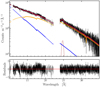 |
Fig. 1 Broadband best-fit to the X-ray spectrum of 4U 1820-30 with warm and cold absorption described in Sect. 3. We display only RGS1 and RGS2 (in grey and black, respectively) of obsID 008411 for clarity. We overlap the best model of the broadband spectrum (in red), which is made up of a Comptonisation model (in blue), and a blackbody (in orange). We also show the Gaussian (in brown) added to the model in order to fit the possible instrumental bump in excess centred at 24.7 Å. We divide the data for the instrumental effective area in order to clean the spectrum from the numerous instrumental features. Bottom panel: residuals defined as (observation-model)/error. |
Best-fit parameters of our model for the broadband spectrum of 4U 1820-30.
4 High-ionisation lines
The spectra of 4U 1820-30 display several lines from highly ionised elements: Mg XI, Ne IX, Fe XVII, O VII, and O VIII. In Table 3, we list all the lines with their detection significance. The effective area of RGS and LETG HRC should allow us to detect the absorption lines of C VI, N VI, and N VII. However, because the cold-gas absorption of the continuum is severe in this region, the signal-to-noise ratio is too low for a meaningful analysis.
These lines are produced by ionised plasma present along the line of sight of the source. To reveal the nature of this ionised gas we study the associated absorption features through two different physical models defined by us as ism and photo models:
ism model – To model the absorption by the hot coronal gas in the ISM we use the collisionally ionised plasma model hot with a temperature above 105.5 K (E ≳ 0.05 keV).
photo model – To investigate the occurrence of photoionised gas intrinsic to the binary, we adopt the xabs model in SPEX (Steenbrugge et al. 2003). The xabs model calculates the transmission through a slab of photoionised gas where all ionic column densities arelinked in a physically consistent fashion through a photoionisation model. To compute the ionisation balance for the xabs model, we use the photoionisation model of SPEX, called PION (Mehdipour et al. 2016). This was done for each dataset independently. For this calculation we adopt the proto-solar abundances of Lodders (2010). We retrieve the spectral energy distribution (SED) for each dataset, normalising the SED of C12 to the soft X-ray band of the observations. In this energy band, the spectral shape remains consistent and only the normalisation varies. As our observations do not cover the hard X-ray band, we assume that the shape of the SED does not vary and remains consistent with that of the SED of C12. The PION calculations yield temperature and ionic column densities as a function of the ionisation parameter ξ (Tarter et al. 1969), which are used for fitting with the xabs model. The ionisation state of the absorber is measured through the ionisation parameter, which is defined as:
Comparison of the photo-ionised and collisional-ionised best-fit model parameters obtained through the C-statistic analysis.
 (1)
(1)
where Lion is the source ionisation luminosity between 1 and 1000 Ryd, nH the hydrogen density of the absorber, and r its distance from the ionising source.
We fit the two models using two different approaches: first the C-statistic, widely used in X-ray data analysis, and then the Bayesian parameter inference (Gregory 2005; Gelman et al. 2013). The C-statistic can have some difficulty identifying multiple, separate, adequate solutions (i.e. local probability maxima) in the parameter space. On the contrary, the Bayesian approach explores the entire parameter space identifying the subvolumes that constitute the bulk of the probability. Moreover, it performs optimisation and error estimation simultaneously, but requires large computation time depending on the number of free parameters. For each model, we evaluate the equivalent hydrogen column density (NH), the flow- (v) and turbulence-velocities (σv or velocity dispersion) of the absorber, together with the temperature (kB T) or the ionisation parameter (ξ), depending on the model.
High-ionisation lines detected in the XMM-Newton and Chandra spectrum.
4.1 C-statistic analysis
For each dataset, we apply the ism and photo models to the broadband continuum model separately. We constrain all the free parameters of the broadband fit to within 1σ uncertainties. We leave only the normalisations of the blackbody and Comptonisation components free to vary (see Sect. 2). We then fit the hot and xabs parameters separately for each dataset and report their best values in Table 4 with the relative uncertainties.
For each epoch, a collisionally ionised gas with an average temperature of 0.16 ± 0.01 keV (1.9 ± 0.1 × 10⁶ K) better represents (with a total ΔCstat = 312) the high-ionisation absorption lines than a photoionised gas with an average ionisation parameter log ξ = 1.72 ± 0.05. We do not observe any significant flow velocity (v) associated to the absorber. The estimates of v are indeed consistent within the uncertainties with a static gas. For RGS and LETG observations, we fix the turbulent velocities to their default value of 100 km s−1 to tackle the degeneration between the fit parameters (in particular between σv and NH). Only with HETG are we able to resolve the turbulent and flow velocities of the absorber. Moreover, the tabulated parameters, such as temperature and NH, do not showsignificant variability among the different epochs, as shown in Fig. 2.
Furthermore, we fit the high-ionisation lines with both the ism and photo models to test the possible coexistence of photoionised and collisionally ionised gases along the line of sight. In this scenario the ism-model dominates the fit and the contribution of the photoionised gas is negligible for each epoch analysed. The coexistence of the two absorbers is not strongly supported by the C-statistics. For the ism + photo model, we find a C-stat/d.o.f. = 27032/21906 with a tiny improvement in the C-stat (ΔC = 8) with respect to the fit with the ism model alone.
4.2 Bayesian analysis
For the spectral analysis using the Bayesian approach (Bayes 1763), we adopt the MultiNest algorithm (version 3.10, Feroz et al. 2009, 2013). This method is applicable to low-dimensional problems of X-ray spectral modelling; its strength is its capability to identify local maxima without difficulty, computing points of equal weighting similar to a Markov chain. It provides values, errorestimates, and marginal probability distributions for each parameter.
To connect the X-ray-fitting code SPEX with the Bayesian methodology, we create a Python package BAYSPEX6, which is a simplified and adapted version of the PyMultiNest and Bayesian X-ray Analysis (BXA) developed by Buchner et al. (2014). This script is adapted to PYSPEX, the python interface to SPEX. The logic behind the script is that MultiNest suggests parameters on a unit hypercube which are translated into model parameters readable by SPEX using the prior definitions. At this point, BAYSPEX computes a probability using the SPEX likelihood implementation, which is passed back to the MultiNest algorithm.
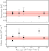 |
Fig. 2 Temperature and hydrogen column density of the ism-model versus the 0.5−2 keV unabsorbed flux for each dataset using the C-statistic fitting model. The horizontal red line represents the inverse-variance-weighted average and the coloured band indicates the 3σ confidence band. Only RGS 008411 (the observation with a flux ~2.2 × 10⁻⁹ erg cm−2 s−1) shows a deviating column density value. |
4.2.1 Parameter inference
Similar to the C-statistic approach, we separately multiply the broadband continuum fit with the ism and photo models. To minimise the number of the free parameters in the fit, we freeze the broadband continuum shape calculated in Sect. 3. Furthermore, we impose the parameters of the ism model to be the same for all the datasets. Instead, for the photo model, we fit the ionisation parameters of the different epochs separately, because each dataset uses a different SED. We couple the velocities and the hydrogen column density to keep the model simple. The Bayesian data analysis is indeed limited by the computation power and time. Moreover, these arrangements are justified by the previous C-statistic analysis. The hot and xabs components do not modify the shape of the broadband model and their parameters are constant along all the epochs (see Table 4).
Figures 3 and 4 display the normalised probability distributions of the ism and photo model parameters, respectively, computed through the Bayesian parameter inference. The estimated values with their errors are reported at the top of each panel. We also illustrate the two-dimensional distribution of the probability pairing the free parameters with each other. In neither of the fits do we observe any strong covariance between the free parameters. Only the ionisation parameters (ξ) and the hydrogen column density of the absorber show a weak correlation visible in the log ξ − logNH plots of Fig. 4.
We also test the coexistence of collisionally ionised and photoionised gases along the line of sight, fitting together the two models (ism+photo model). As the Bayesian approach explores the full parameter space, it can return more statistically robust results than the C-stat. We show the probability distribution of the parameters for these models in Fig. 5. As an example, we show the ionisation parameter of observation 008411. While the parameters of the hot component (the four upper distributions) are well defined, the xabs quantities (the four lower distributions) are not constrained. Only the relative column density shows a peaked probability distribution indicating that the fraction of the possible photoionisation gas in modelling the high-ionisation lines is very small (less than 0.002).
Moreover, we investigate whether or not multiple-temperature interstellar hot gas (ism+ism model) or multiple photoionised gases (photo + photo model) can better describe the absorption features. In both cases we find that a single gaseous component dominates the fit and the contribution of a secondary absorber can be considered negligible.
To decipher which candidate among the ism, photo, ism + photo, ism + ism, and photo + photo models best fits the high-ionisation lines of 4U 1820-30, we compute the Bayesian model analysis presented in the following section.
4.2.2 Model comparison
Bayesian model comparison is done by comparing models on the basis of the posterior probability of the model given the data, known as Bayesian evidence. Using Bayes’s rule, the Bayesian evidence (Z) is proportional to the prior probability for the model, p(M), multiplied by the likelihood of the data (y) given the model, p(y|M). The choice between two models, M1 and M2, can be made on the basis of the ratio of their Bayesian evidences. This ratio is known as Bayes factor (B1,2, Wasserman 2000; Liddle 2007; Trotta 2008; Knuth et al. 2014). As we choose uniform priors for different models in our analysis, the Bayes factor is defined as:
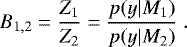 (2)
(2)
A large value of this ratio gives support for M1 over M2. Specifically, we adopt the scale of Jeffreys (1961) and we rule out models that show B1,2 > 30 (log B1,2 > 1.5). A Bayes factor above 30 represents “very strong evidence” against M2. The strength of this method is that it does not require models to be nested (i.e. M2 as a special case of M1), nor does it make assumptions about the parameter space or the data. Moreover, it automatically introduces a penalty for including too much model complexity, guarding against overfitting the data (Kass & Raftery 1995).
The Bayesian statistics includes an approximation to the Bayesian evidence known as the Bayesian information criterion (BIC, Schwarz 1978) which is defined as  , where
  is the maximum likelihood, k the number of parameters of the model, and N the number of data points used in the fit.
An alternative model comparison consists in the information-theoretic methods, pioneered by Akaike (1974) with his Akaike information criterion (AIC), which is defined as  . Similarly to the Bayesian model selection, AIC and BIC can be used to decide which model is more likely to have produced the data: the most probable model corresponds to the fit with the smallest AIC and BIC value, respectively. Both AIC and BIC include an over-fitting term by which the more complex models are disfavoured by the additional number of parameters. A description geared to astronomers can be found in Takeuchi (2000) and Liddle (2004), while the full statistical procedure can be found in Burnham & Anderson (2002).
We compare all the models presented in Sect. 4.2.1 (ism, photo, ism + photo, ism + ism, and photo + photo) using the Bayesian evidence. We list the results of the model comparison in Table 5, where we also report the relative AIC and BIC values. An interstellar hot gas with a single temperature is the favourite scenario for describing the high-ionisation lines observed in the spectra of 4U 1820-30. The result of the Bayesian analysis is therefore in agreement with the outcome of the C-statistic (see Sect. 4.1).
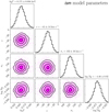 |
Fig. 3 Posterior distribution from MultiNest plotted with two-dimensional histograms comparing each pair of free parameters hot-model (NH, kB T, v and σv). The contours indicate the 1σ, 2σ, 3σ, and 4σ confidence intervals in two-dimensional space. The hydrogen column density NH is expressed in units of 1024 cm−2. |
5 Discussion
In order to determine the origin of the high-ionisation absorption lines observed in the spectra of 4U 1820-30, we fit them adopting both photo-ionisation and collisional-ionisation models. In Fig. 6, we compare the fits of the two models obtained through the Bayesian parameter inference. The ism model reproduces all the lines better than the photo model, in particular the Fe XVII which is detected with a significance of 6.5σ. This line was detected by Yao et al. (2006) and Luo & Fang (2014). Whereas the former authors propose an interstellar origin for this line, the latter authors conclude that the majority of the Fe XVII line arises from an intrinsic gas to the source. In our analysis, we noticed that the photo-model does not describe the Fe XVII line (see Fig. 6) because the fraction of the ion according to the photo-ionised model is very low.
In Fig. 7, we plot the ionisation fractions of the ionised atoms for which we detected the lines in the spectrum. In particular, we show the relative column densities of both models. The different distributions of the column densities of the ions are crucial to selecting which model best fits the spectral features. For a photoionised gas with a mild photoionisation parameter (log ξ ~ 1.8), iron is divided into multiple ionisation states. Consequently, the ionisation fraction of each individual Fe ion becomes low. Instead, for a collisionally ionised gas, the column densities are distributed differently: the ionisation fraction is more peaked at the preferred ionisation state, which is determined by the temperature of the gas. Therefore, the detection of the Fe XVII line suggests an interstellar nature for the high-ionisation lines.
However, the photoionisation nature is statistically ruled out (see Table 5). All the three model comparison criteria considered indicate the ism as the preferred model. The evidence against the ism + photo model is particularly strong with the BIC criterion which severely penalises complex models. In Table 6 we list the values of the parameters obtained with Bayesian analysis. In the following, we discuss the results obtained for the ism and photo models in detail.
Model selection results for 4U 1820-30.
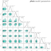 |
Fig. 4 Posterior distribution from MultiNest is plotted with two-dimensional histograms comparing each pair of free parameters of the xabs-model (NH, v, σv, and the logξ for each observation; the number of each observation is indicated in the distribution panel). The contours indicate the 1σ, 2σ, 3σ, and 4σ confidence intervals in two-dimensional space. The hydrogen column density NH is expressed in units of 1024 cm−2. |
5.1 Photoionisation origin
Both Bayesian and C-statistic approaches indicate that photoionisation model is less able to fit the spectra of 4U 1820-30 with respect to the collision–ionisation model. The absorber is found to have a low outflow velocity which does not support the presence of a disc wind. This velocity has to be corrected for the Solar System barycentric radial velocity of the satellite. During all the HETG observations (obsid 1021, 1022, 6633, and 6634, 7032) this velocity was vbar ~ 30 km s−1, which explains the low outflow velocity observed. Due to its high energy resolution, the HETG instrument puts more stringent constraints on a possible flow velocity.
Moreover, the presence of a local ionised gas, such as a disc atmosphere, would be difficult to justify given the physical parameters of the source. Through the ionisation parameter, we can calculate the density, nH, if one knows where the plasma is located with respect to the X-ray source. Taking an ionising luminosity of Lion = 8 × 1037 erg s−1 (computed using the SED of C12, for the range 1–1000 Ryd), a distance r < 1.3 × 10¹⁰ (which corresponds to the size of the system, Stella et al. 1987), and an ionisation parameter of ξ = 62 erg s−1 cm (Sect. 4.2), the density of the plasma must be n > 7 × 1015 cm−3, which is some orders of magnitude larger than the density of the typical disc atmosphere of a low-mass X-ray binary system (e.g. van Peet et al. 2009). This large density value would also imply that the filling factor, f =NH∕nr, is extremely low f < 4 × 10⁻⁷, with NH= 3.9 × 1019 cm−2. Cackett et al. (2008) argued that a proper physical solution for such a small filling factor is the presence of dense structures above the disc, such as high-density blobs, produced by thermal instabilities. For example, dense clumps, possibly part of the accretion bulge observed in dipping sources, have been observed (e.g. Psaradaki et al. 2018). However, their density is nH ~ 1013 cm−3, which is two orders of magnitude lower than the density expected for a possible locally photoionised material. Another argument against a photoionisation origin is the lack of variability of the lines observed among the different epochs (Fig. 2 and Cackett et al. 2008).
However, the fact that the collisional–ionisation model best represents the ionised lines of the spectra may not exclude the existence of a second component intrinsic to the source. Thus, to test the possible presence of this photo-ionised gas beside the hot interstellar plasma we compute a fit using both models. Our analysis, in particular the C-statistic, shows that there is no significant contribution from photo-ionised gas towards the source for the epochs covered by the observations. Furthermore, the Bayesian parameter inference shows a negligible column density of the photo-ionised gas (see Fig. 5).
One question that arises asks why we do not detect any significant absorption lines from a photoionised wind/atmosphere intrinsic to 4U 1820-30. Considering the SED of the ionisation source and the small size of the system, the disc and/or atmosphere could be fully ionised, making it impossible to detect any absorption lines (Stella et al. 1987; Futamoto et al. 2004). Yet the inclination angle of the system can be a crucial factor for the non-detection of photoionised lines. Díaz Trigo & Boirin (2016) showed that the preferential detection of absorbing photoionised plasma is for a system with a relative high (i > 50°) inclination. The lower inclination of the 4U 1820-30 ( , Anderson et al. 1997) system may imprint absorption lines that are too weak to be detected, as our line of sight would go through a thinner layer of gas.
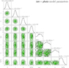 |
Fig. 5 Posterior distribution from MultiNest plotted with two-dimensional histograms comparing each pair of free parameters of the hot-model (NH, kB T, v and σv) in the four upper distributions, together with the free parameters of the xabs-model (NH, v, σv and log ξ; for clarity, we show only the logξ of observation 008411) in the four lower distributions. The contours indicate the 1σ, 2σ, 3σ, and 4σ confidence intervals in two-dimensional space. The hydrogen column densities NH are expressed in units of 1024cm−2. |
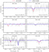 |
Fig. 6 High-ionisation lines detected in the spectra of 4U 1820-30. Here, the spectrum is shown in units of transmittance: the observed counts are divided by the underlying continuum together with the cold and warm absorption. For clarity, we do not display all the datasets. We superimpose the ism and photo models (in red and blue, respectively) obtained with the Bayesian parameter inference. |
5.2 Interstellar origin
A single-temperature hot gas can describe the absorption lines well. Specifically, we observe a gas with a temperature of ~ 1.98 × 10⁶ K, which is consistent with the values obtained in previous studies (e.g. Yao et al. 2006) and with the temperature observed for several Galactic low-mass X-ray binaries (Yao & Wang 2005). Furthermore, we tested the presence of multiple-temperature gases, adding a supplementary hot component. One may expect variation in the physical and possibly also chemical properties of the hot gas along the line of sight to 4U 1820-30 which crosses several bubbles such as the Local Bubble around the Sun (with T ~ 106 K, Kuntz & Snowden 2000) and Loop I Bubble (with T ~ 3.5 × 10⁶ K, Miller et al. 2008). However, from our modelling we do not find multiple gases with different temperatures. The opacity of the gas contained in local bubbles is too low to be detected in the spectrum. Therefore, for the line of sight towards 4U 1820-30, we assume a single hot plasma component which is consistent with the scenario suggested by Hagihara et al. (2011). In addition, this uniform hot coronal gas is also in agreement with the presence of a hot and thick interstellar disc, as suggested by observations of extragalactic sources (Yao et al. 2009; Hagihara et al. 2010).
Through the Bayesian data analysis we are able to evaluate the velocity dispersion of the hot coronal gas, σv = 132 ± 16 km s-1. Constraining this quantity is not trivial and a proper collisional ionisation equilibrium model is necessary. Yao & Wang (2006) found a dispersion velocity7 between 117 and 262 km s-1 for the hot gas along the line of sight towards 4U 1820-30. Our velocity dispersion estimate is also in agreement with the dispersion velocities observed from the survey of the O VI (σv = 50−200 km s-1) with the FarUltraViolet Spectroscopic Explorer, FUSE (Otte & Dixon 2006). The O VI line is often used as a tracer of gas with a peak temperatureof T ≈ 3 × 10⁵ K. Such intermediate-temperature gas is expected primarily at the interface between the cool/warm clouds and the hot coronal gas (Sembach et al. 2003). Finally, similar values of velocity dispersion and flow velocity were found by Luo et al. (2018), who analysed the O VII absorption line.
For a collisionally ionised gas with a temperature of T ~1.98 × 10⁶ K, the expected thermal broadening is  . This value is too low to explain the observed velocity dispersion. This velocity cannot be accounted for by differential Galactic rotation either. The lines are indeed far wider than expected if the absorption came from a smoothly distributed ISM corotating with the disc of the Milky Way (Bowen et al. 2008). The observed velocity dispersion instead supports the picture of a turbulent hot coronal gas mixed up by shock-heated gas from multiple supernova explosions. The numerical simulations of de Avillez & Breitschwerdt (2005) show hot gas arises in bubbles around supernovae, which is then sheared through turbulent diffusion, destroying the bubbles and stretching the hot absorbing gas into filaments and vortices that dissipate with time. Furthermore, the hot gas is involved in systematic vertical motion as it streams to the halo at a speed of 100−200 km s-1. This kinetic energy can be transformed into disordered, turbulent motions, resulting in higher turbulent velocities near the halo (Kalberla et al. 1998).
Comparing the hydrogen column densities of the different components detected along the line of sight of the source, we observe the following gas mass fraction: cold ~89%, warm ~8%, and hot ~3%. These values are very similar to the mass fractions found by Gatuzz & Churazov (2018) for 4U 1820-30 (85, 10 and 5%) and they agree with findings for different lines of sight of Galactic sources. For example, Pinto et al. (2013), analysing the high-resolution X-ray spectra of a sample of Galactic X-ray binaries, found that on average the ~ 90, ~ 7, and ~ 3% of the ISM mass correspond to a cold, warm, hot plasma, respectively.
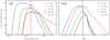 |
Fig. 7 Ionisation fractions of oxygen, neon, magnesium, and iron ions as a function of the electron temperature for collisional ionisation equilibrium plasma (CIE, ism-model on the left panel) and as a function of the ionisation parameter for a gas in photoionisation equilibrium (PIE, photo-model, on the right panel). The vertical dashed lines indicate the best values for kB T and ξ (observation008411) obtained through the Bayesian analysis. |
Parameter values estimated through the Bayesian analysis.
5.3 Abundances of the hot coronal gas
We further investigated the abundances of oxygen, neon, magnesium, and iron for the hot phase of the ISM. For these elements, we detect high-ionisation lines. Using the Bayesian parameter inference we obtain abundances close to their protosolar values: AO = 0.90 ± 0.06 A⊙, ANe = 1.16 ± 0.08 A⊙, AMg = 1.9 ± 0.4 A⊙, and AFe = 1.07 ± 0.11 A⊙, keeping the abundances tabulated in Lodders (2010) as references.
The hot phase abundances of oxygen and neon are consistent with the characteristic depletion of these elements in the ISM. As neon is a noble element, it is very unlikely to be depleted in dust grains in all the medium phases and oxygen shows low depletion values in the ISM (Jenkins 2009). Iron and magnesium are instead highly depleted from the gas phase in the ISM (e.g. Jenkins 2009; Rogantini et al. 2018, 2019, 2020). The depletion of iron in particular remains high even in harsh environments (Whittet 2002). However, the observed abundances for magnesium and iron suggests that in the hot coronal gas along the line of sight towards 4U 1820-30, these two elements are mostly present in the gas phase. This supports the scenario where all the interstellar dust in this very hot phase (T ≳ 105.5 K) is destroyed by frequent shocks during the dust grain processing in the ISM. This interpretation may not be entirely unique. Reports of an overabundance of heavier elements relative to oxygen in neutral matter toward the Galacticcentre might suggest an elevation of the contribution of these elements in the hot phase as well. A comparison with different lines of sight, especially towards sources at high latitudes, is therefore essential before drawing conclusions.
6 Summary
Motivated by defining the origin of the high-ionisation absorption features present in the spectrum of the ultracompact system 4U 1820-30, we systematically analysed all the observations present in the Chandra and XMM-Newton archives: five Chandra/HETG spectra together with two Chandra /LETG and two XMM-Newton /RGS observations. We study the soft X-ray energy band covering the main high-ionisation absorption lines: namely, Mg XI, Ne IX, Fe XVII, O VII Heα, O VII Heβ, O VIII Lyα and O VIII Lyβ. We adopt realistic plasma models to fit the multiple lines simultaneously: in particular we use the SPEX model xabs to reproduce a photo-ionised gas and hot for a thermal gas in a collisional ionised equilibrium state. We used a Bayesian framework to model the spectral absorption features. Bayesian data analysis provides a robust approach to infer the model parameters and their uncertainties and offers a solid model comparison.
Both the C-statistic and Bayesian data analysis show the presence of hot coronal gas with a temperature of T ~ 1.98 × 10⁶ K (kBT = 0.171 ± 0.004 keV) along the line of sight towards 4U 1820-30. This hot interstellar gas is responsible for the high-ionisation absorption lines detected in the spectra. We summarise our main results as follows:
-
The mean centroids of the absorption lines are consistent with their rest-frame wavelengths. The low line-of-sight velocity observed is within the uncertainty due to the dynamic radial velocity of the observer. As concluded by previous works (e.g. Futamoto et al. 2004), an outflowing disc wind can be ruled out as possible ionised absorber.
-
The lack of variability of the lines through the multiple observations also shows that the absorber is independent from the activity of the source, suggesting a non-local origin for the gas.
-
In the spectra of 4U 1820-30 we detect the Fe XVII line at 15.012 Åwith a significance of 6.5σ. This line is best reproduced by a gas in collisional ionisation equilibrium. In contrast, for an absorber photoionised by the source, the contribution of Fe XVII is not high enough to justify the strength of the absorption line detected.
-
We constrain the turbulent velocity of the hot gas to be σv = 132 ± 16 km s-1 which is likely driven by supernova shock-waves.
Acknowledgements
We would like to thank the anonymous referee for the useful suggestions. D.R., E.C., and M.M. are supported by the Netherlands Organisation for Scientific Research (NWO) through The Innovational Research Incentives Scheme Vidi grant 639.042.525. The Space Research Organization of the Netherlands is supported financially by NWO. This research has made use of data obtained from the Chandra Transmission Grating Catalog and archive (http://tgcat.mit.edu), and software provided by the Chandra X-ray Center in the application package CIAO. We also made used of the XMM-Newton Scientific Analysis System developed by a team of scientist located at ESA’s XMM-Newton Science Operations Centre and at the XMM-Newton Survey Science Centre. We are grateful to M. Díaz Trigo for a useful discussion on the photoionised atmosphere of 4U 1820-30. We thank A. Dekker and D. Lena for reading an early draft of the manuscript and for providing valuable comments and suggestions. We also thank I. Psaradaki for her input on the XMM-Newton data reduction and J. de Plaa for his support on the development of the program.
References
- Akaike, H. 1974, IEEE Trans. Auto. Control, 19, 716 [Google Scholar]
- Anderson, S. F., Margon, B., Deutsch, E. W., Downes, R. A., & Allen, R. G. 1997, ApJ, 482, L69 [NASA ADS] [CrossRef] [Google Scholar]
- Arnaud, K. A. 1996, ASP Conf. Ser., 101, 17 [Google Scholar]
- Bautista, M. A., & Kallman, T. R. 2001, ApJS, 134, 139 [NASA ADS] [CrossRef] [Google Scholar]
- Bayes, T. 1763, Phil. Trans. R. Soc. London, 53, 370 [Google Scholar]
- Bowen, D. V., Jenkins, E. B., Tripp, T. M., et al. 2008, ApJS, 176, 59 [NASA ADS] [CrossRef] [Google Scholar]
- Brinkman, B. C., Gunsing, T., Kaastra, J. S., et al. 2000, SPIE Conf. Ser., 4012, 81 [Google Scholar]
- Buchner, J., Georgakakis, A., Nandra, K., et al. 2014, A&A, 564, A125 [NASA ADS] [CrossRef] [EDP Sciences] [Google Scholar]
- Burnham, K. P., & Anderson, D. R. 2002, Model Selection and Multimodel Inference: A Practical Information-Theoretic Approach, 2nd edn. (Berlin: Springer), 1 [Google Scholar]
- Cackett, E. M., Miller, J. M., Raymond, J., et al. 2008, ApJ, 677, 1233 [NASA ADS] [CrossRef] [Google Scholar]
- Canizares, C. R., Davis, J. E., Dewey, D., et al. 2005, PASP, 117, 1144 [NASA ADS] [CrossRef] [Google Scholar]
- Cash, W. 1979, ApJ, 228, 939 [NASA ADS] [CrossRef] [Google Scholar]
- Corrales, L. R., García, J., Wilms, J., & Baganoff, F. 2016, MNRAS, 458, 1345 [NASA ADS] [CrossRef] [Google Scholar]
- Costantini, E., Pinto, C., Kaastra, J. S., et al. 2012, A&A, 539, A32 [NASA ADS] [CrossRef] [EDP Sciences] [Google Scholar]
- de Avillez, M. A., & Breitschwerdt, D. 2005, ApJ, 634, L65 [NASA ADS] [CrossRef] [Google Scholar]
- den Herder, J. W., Brinkman, A. C., Kahn, S. M., et al. 2001, A&A, 365, L7 [NASA ADS] [CrossRef] [EDP Sciences] [Google Scholar]
- de Plaa, J., Kaastra, J. S., Tamura, T., et al. 2004, A&A, 423, 49 [NASA ADS] [CrossRef] [EDP Sciences] [Google Scholar]
- Díaz Trigo, M., & Boirin, L. 2016, Astron. Nachr., 337, 368 [NASA ADS] [CrossRef] [Google Scholar]
- Díaz Trigo, M., Parmar, A. N., Boirin, L., Méndez, M., & Kaastra, J. S. 2006, A&A, 445, 179 [NASA ADS] [CrossRef] [EDP Sciences] [Google Scholar]
- Feroz, F., Hobson, M. P., & Bridges, M. 2009, MNRAS, 398, 1601 [NASA ADS] [CrossRef] [Google Scholar]
- Feroz, F., Hobson, M. P., Cameron, E., & Pettitt, A. N. 2013, Open J. Astrophys., 2 [Google Scholar]
- Ferrière, K. M. 2001, Rev. Mod. Phys., 73, 1031 [NASA ADS] [CrossRef] [Google Scholar]
- Fruscione, A., McDowell, J. C., Allen, G. E., et al. 2006, Proc. SPIE, 6270, 62701V [Google Scholar]
- Futamoto, K., Mitsuda, K., Takei, Y., Fujimoto, R., & Yamasaki, N. Y. 2004, ApJ, 605, 793 [NASA ADS] [CrossRef] [Google Scholar]
- Gatuzz, E., & Churazov, E. 2018, MNRAS, 474, 696 [CrossRef] [Google Scholar]
- Gelman, A., Carlin, J., Stern, H., et al. 2013, Bayesian Data Analysis, 3rd edn., Chapman & Hall/CRC Texts in Statistical Science (Taylor & Francis) [Google Scholar]
- Giacconi, R., Murray, S., Gursky, H., et al. 1972, ApJ, 178, 281 [NASA ADS] [CrossRef] [Google Scholar]
- Gorczyca, T. W. 2000, Phys. Rev. A, 61, 024702 [NASA ADS] [CrossRef] [Google Scholar]
- Gregory, P. C. 2005, Bayesian Logical Data Analysis for the Physical Sciences: A Comparative Approach with ‘Mathematica’ Support (Cambridge: Cambridge University Press) [Google Scholar]
- Hagihara, T., Yao, Y., Yamasaki, N. Y., et al. 2010, PASJ, 62, 723 [NASA ADS] [Google Scholar]
- Hagihara, T., Yamasaki, N. Y., Mitsuda, K., et al. 2011, PASJ, 63, S889 [NASA ADS] [CrossRef] [Google Scholar]
- Huenemoerder, D. P., Mitschang, A., Dewey, D., et al. 2011, AJ, 141, 129 [NASA ADS] [CrossRef] [Google Scholar]
- Jeffreys, H. 1961, Theory of Probability, 3rd edn. (Oxford, England: Oxford University Press) [Google Scholar]
- Jenkins, E. B. 1978, ApJ, 219, 845 [NASA ADS] [CrossRef] [Google Scholar]
- Jenkins, E. B. 2009, ApJ, 700, 1299 [NASA ADS] [CrossRef] [Google Scholar]
- Juett, A. M., Schulz, N. S., & Chakrabarty, D. 2004, ApJ, 612, 308 [NASA ADS] [CrossRef] [Google Scholar]
- Juett, A. M., Schulz, N. S., Chakrabarty, D., & Gorczyca, T. W. 2006, ApJ, 648, 1066 [NASA ADS] [CrossRef] [Google Scholar]
- Kaastra, J. S., Raassen, A. J. J., de Plaa, J., & Gu, L. 2018, SPEX X-ray spectral fitting package [Google Scholar]
- Kalberla, P. M. W., Westphalen, G., Mebold, U., Hartmann, D., & Burton, W. B. 1998, A&A, 332, L61 [NASA ADS] [Google Scholar]
- Kass, R. E., & Raftery, A. E. 1995, J. Am. Stat. Assoc., 90, 773 [CrossRef] [Google Scholar]
- Kirchhoff, G., & Bunsen, R. 1860, Ann. Phys., 186, 161 [NASA ADS] [CrossRef] [Google Scholar]
- Knuth, K. H., Habeck, M., Malakar, N. K., Mubeen, A. M., & Placek, B. 2014, Digit. Signal Process., 47, 50 [CrossRef] [Google Scholar]
- Kortright, J. B., & Kim, S.-K. 2000, Phys. Rev. B, 62, 12216 [NASA ADS] [CrossRef] [Google Scholar]
- Kuntz, K. D., & Snowden, S. L. 2000, ApJ, 543, 195 [NASA ADS] [CrossRef] [Google Scholar]
- Kuulkers, E., den Hartog, P. R., in’t Zand, J. J. M., et al. 2003, A&A, 399, 663 [NASA ADS] [CrossRef] [EDP Sciences] [Google Scholar]
- Lee, J. C., Reynolds, C. S., Remillard, R., et al. 2002, ApJ, 567, 1102 [NASA ADS] [CrossRef] [Google Scholar]
- Liao, J.-Y., Zhang, S.-N., & Yao, Y. 2013, ApJ, 774, 116 [NASA ADS] [CrossRef] [Google Scholar]
- Liddle, A. R. 2004, MNRAS, 351, L49 [NASA ADS] [CrossRef] [Google Scholar]
- Liddle, A. R. 2007, MNRAS, 377, L74 [NASA ADS] [Google Scholar]
- Lodders, K. 2010, Astrophys. Space Sci. Proc., 16, 379 [NASA ADS] [CrossRef] [Google Scholar]
- Luo, Y., & Fang, T. 2014, ApJ, 780, 170 [NASA ADS] [CrossRef] [Google Scholar]
- Luo, Y., Fang,T., & Ma, R. 2018, ApJS, 235, 28 [CrossRef] [Google Scholar]
- McKee, C. F.,& Ostriker, J. P. 1977, ApJ, 218, 148 [NASA ADS] [CrossRef] [Google Scholar]
- Mehdipour, M., Kaastra, J. S., & Kallman, T. 2016, A&A, 596, A65 [NASA ADS] [CrossRef] [EDP Sciences] [Google Scholar]
- Miller, M. J., & Bregman, J. N. 2013, ApJ, 770, 118 [NASA ADS] [CrossRef] [Google Scholar]
- Miller, E. D., Tsunemi Hiroshi, Bautz, M. W., et al. 2008, PASJ, 60, S95 [CrossRef] [Google Scholar]
- Miller, J. M., Cackett, E. M., & Reis, R. C. 2009, ApJ, 707, L77 [NASA ADS] [CrossRef] [Google Scholar]
- Nicastro, F., Mathur, S., Elvis, M., et al. 2005, Nature, 433, 495 [NASA ADS] [CrossRef] [PubMed] [Google Scholar]
- Otte, B., & Dixon, W. V. D. 2006, ApJ, 647, 312 [CrossRef] [Google Scholar]
- Parmar, A. N., Oosterbroek, T., Boirin, L., & Lumb, D. 2002, A&A, 386, 910 [NASA ADS] [CrossRef] [EDP Sciences] [Google Scholar]
- Pinto, C., Kaastra, J. S., Costantini, E., & Verbunt, F. 2010, A&A, 521, A79 [NASA ADS] [CrossRef] [EDP Sciences] [Google Scholar]
- Pinto, C., Kaastra, J. S., Costantini, E., & de Vries, C. 2013, A&A, 551, A25 [NASA ADS] [CrossRef] [EDP Sciences] [Google Scholar]
- Psaradaki, I., Costantini, E., Mehdipour, M., & Díaz Trigo, M. 2018, A&A, 620, A129 [NASA ADS] [CrossRef] [EDP Sciences] [Google Scholar]
- Rogantini, D., Costantini, E., Zeegers, S. T., et al. 2018, A&A, 609, A22 [NASA ADS] [CrossRef] [EDP Sciences] [Google Scholar]
- Rogantini, D., Costantini, E., Zeegers, S. T., et al. 2019, A&A, 630, A143 [CrossRef] [EDP Sciences] [Google Scholar]
- Rogantini, D., Costantini, E., Zeegers, S. T., et al. 2020, A&A, 641, A149 [CrossRef] [EDP Sciences] [Google Scholar]
- Schwarz, G. 1978, Ann. Stat., 6, 461 [Google Scholar]
- Sembach, K. R., Wakker, B. P., Savage, B. D., et al. 2003, ApJS, 146, 165 [NASA ADS] [CrossRef] [Google Scholar]
- Sidoli, L., Oosterbroek, T., Parmar, A. N., Lumb, D., & Erd, C. 2001a, A&A, 379, 540 [NASA ADS] [CrossRef] [EDP Sciences] [Google Scholar]
- Sidoli, L., Parmar, A. N., Oosterbroek, T., et al. 2001b, A&A, 368, 451 [NASA ADS] [CrossRef] [EDP Sciences] [Google Scholar]
- Steenbrugge, K. C., Kaastra, J. S., de Vries, C. P., & Edelson, R. 2003, A&A, 402, 477 [NASA ADS] [CrossRef] [EDP Sciences] [Google Scholar]
- Steenbrugge, K. C., Kaastra, J. S., Crenshaw, D. M., et al. 2005, A&A, 434, 569 [NASA ADS] [CrossRef] [EDP Sciences] [Google Scholar]
- Stella, L., Priedhorsky, W., & White, N. E. 1987, ApJ, 312, L17 [NASA ADS] [CrossRef] [Google Scholar]
- Takeuchi, T. T. 2000, Ap&SS, 271, 213 [NASA ADS] [CrossRef] [Google Scholar]
- Tanaka, Y., & Bleeker, J. A. M. 1977, Space Sci. Rev., 20, 815 [NASA ADS] [CrossRef] [Google Scholar]
- Tarter, C. B., Tucker, W. H., & Salpeter, E. E. 1969, ApJ, 156, 943 [NASA ADS] [CrossRef] [Google Scholar]
- Titarchuk, L. 1994, ApJ, 434, 570 [NASA ADS] [CrossRef] [Google Scholar]
- Trotta, R. 2008, Contemp. Phys., 49, 71 [Google Scholar]
- Ueda, Y., Murakami, H., Yamaoka, K., Dotani, T., & Ebisawa, K. 2004, ApJ, 609, 325 [NASA ADS] [CrossRef] [Google Scholar]
- van Dyk, D. A., Connors, A., Kashyap, V. L., & Siemiginowska, A. 2001, ApJ, 548, 224 [NASA ADS] [CrossRef] [Google Scholar]
- van Peet, J. C. A., Costantini, E., Méndez, M., Paerels, F. B. S., & Cottam, J. 2009, A&A, 497, 805 [NASA ADS] [CrossRef] [EDP Sciences] [Google Scholar]
- Wang, Q. D. 2010, Proc. Natl. Acad. Sci., 107, 7168 [CrossRef] [Google Scholar]
- Wasserman, L. 2000, J. Math. Psychol., 44, 92 [CrossRef] [Google Scholar]
- Whittet, D. 2002, Dust in the Galactic Environment, 2nd edn., Series in Astronomy and Astrophysics (Taylor & Francis) [Google Scholar]
- Yao, Y., & Wang, Q. D. 2005, ApJ, 624, 751 [NASA ADS] [CrossRef] [Google Scholar]
- Yao, Y., & Wang, Q. D. 2006, ApJ, 641, 930 [NASA ADS] [CrossRef] [Google Scholar]
- Yao, Y., Schulz, N., Wang, Q. D., & Nowak, M. 2006, ApJ, 653, L121 [NASA ADS] [CrossRef] [Google Scholar]
- Yao, Y., Wang, Q. D., Hagihara, T., et al. 2009, ApJ, 690, 143 [NASA ADS] [CrossRef] [Google Scholar]
For the wavelength of the lines we refer to Juett et al. (2006) and the SPEX atomic database Kaastra et al. (2018).
For the wavelength of the photoabsorption edges we refer to Gorczyca (2000) and Kortright & Kim (2000).
BAYSPEX is publicly available on ZenodoLINK.
Yao & Wang (2006) defined the dispersion velocity (bv) as  )
)
All Tables
Observation log of XMM-Newton and Chandra data used for our spectral modelling of 4U 1820-30.
Comparison of the photo-ionised and collisional-ionised best-fit model parameters obtained through the C-statistic analysis.
All Figures
|
Fig. 1 Broadband best-fit to the X-ray spectrum of 4U 1820-30 with warm and cold absorption described in Sect. 3. We display only RGS1 and RGS2 (in grey and black, respectively) of obsID 008411 for clarity. We overlap the best model of the broadband spectrum (in red), which is made up of a Comptonisation model (in blue), and a blackbody (in orange). We also show the Gaussian (in brown) added to the model in order to fit the possible instrumental bump in excess centred at 24.7 Å. We divide the data for the instrumental effective area in order to clean the spectrum from the numerous instrumental features. Bottom panel: residuals defined as (observation-model)/error. |
| In the text | |
|
Fig. 2 Temperature and hydrogen column density of the ism-model versus the 0.5−2 keV unabsorbed flux for each dataset using the C-statistic fitting model. The horizontal red line represents the inverse-variance-weighted average and the coloured band indicates the 3σ confidence band. Only RGS 008411 (the observation with a flux ~2.2 × 10⁻⁹ erg cm−2 s−1) shows a deviating column density value. |
| In the text | |
|
Fig. 3 Posterior distribution from MultiNest plotted with two-dimensional histograms comparing each pair of free parameters hot-model (NH, kB T, v and σv). The contours indicate the 1σ, 2σ, 3σ, and 4σ confidence intervals in two-dimensional space. The hydrogen column density NH is expressed in units of 1024 cm−2. |
| In the text | |
|
Fig. 4 Posterior distribution from MultiNest is plotted with two-dimensional histograms comparing each pair of free parameters of the xabs-model (NH, v, σv, and the logξ for each observation; the number of each observation is indicated in the distribution panel). The contours indicate the 1σ, 2σ, 3σ, and 4σ confidence intervals in two-dimensional space. The hydrogen column density NH is expressed in units of 1024 cm−2. |
| In the text | |
|
Fig. 5 Posterior distribution from MultiNest plotted with two-dimensional histograms comparing each pair of free parameters of the hot-model (NH, kB T, v and σv) in the four upper distributions, together with the free parameters of the xabs-model (NH, v, σv and log ξ; for clarity, we show only the logξ of observation 008411) in the four lower distributions. The contours indicate the 1σ, 2σ, 3σ, and 4σ confidence intervals in two-dimensional space. The hydrogen column densities NH are expressed in units of 1024cm−2. |
| In the text | |
|
Fig. 6 High-ionisation lines detected in the spectra of 4U 1820-30. Here, the spectrum is shown in units of transmittance: the observed counts are divided by the underlying continuum together with the cold and warm absorption. For clarity, we do not display all the datasets. We superimpose the ism and photo models (in red and blue, respectively) obtained with the Bayesian parameter inference. |
| In the text | |
|
Fig. 7 Ionisation fractions of oxygen, neon, magnesium, and iron ions as a function of the electron temperature for collisional ionisation equilibrium plasma (CIE, ism-model on the left panel) and as a function of the ionisation parameter for a gas in photoionisation equilibrium (PIE, photo-model, on the right panel). The vertical dashed lines indicate the best values for kB T and ξ (observation008411) obtained through the Bayesian analysis. |
| In the text | |
Current usage metrics show cumulative count of Article Views (full-text article views including HTML views, PDF and ePub downloads, according to the available data) and Abstracts Views on Vision4Press platform.
Data correspond to usage on the plateform after 2015. The current usage metrics is available 48-96 hours after online publication and is updated daily on week days.
Initial download of the metrics may take a while.