| Issue |
A&A
Volume 644, December 2020
|
|
|---|---|---|
| Article Number | A74 | |
| Number of page(s) | 19 | |
| Section | Interstellar and circumstellar matter | |
| DOI | https://doi.org/10.1051/0004-6361/202039081 | |
| Published online | 02 December 2020 | |
Accretion bursts in magnetized gas-dust protoplanetary disks
1
Department of Astrophysics, University of Vienna,
Vienna,
1180, Austria
e-mail: eduard.vorobiev@univie.ac.at
2
Southern Federal University, Research Institute of Physics,
Rostov-on-Don,
344090
Russia
3
Ural Federal University,
51 Lenin Str.,
620051
Ekaterinburg,
Russia
4
Theoretical Physics Department, Chelyabinsk State University,
454001
Chelyabinsk,
Russia
5
Department of Physics and Astronomy, University of Western Ontario,
London,
Ontario
N6A 3K7, Canada
6
Department of Astronomy, University of Geneva,
Chemin d’Ecogia 16,
1290 Versoix, Switzerland
Received:
1
August
2020
Accepted:
30
October
2020
Aims. Accretion bursts triggered by the magnetorotational instability (MRI) in the innermost disk regions were studied for protoplanetary gas-dust disks that formed from prestellar cores of a various mass Mcore and mass-to-magnetic flux ratio λ.
Methods. Numerical magnetohydrodynamics simulations in the thin-disk limit were employed to study the long-term (~1.0 Myr) evolution of protoplanetary disks with an adaptive turbulent α-parameter, which explicitly depends on the strength of the magnetic field and ionization fraction in the disk. The numerical models also feature the co-evolution of gas and dust, including the back-reaction of dust on gas and dust growth.
Results. A dead zone with a low ionization fraction of x≲10−13 and temperature on the order of several hundred Kelvin forms in the inner disk soon after its formation, extending from several to several tens of astronomical units depending on the model. The dead zone features pronounced dust rings that are formed due to the concentration of grown dust particles in the local pressure maxima. Thermal ionization of alkaline metals in the dead zone trigger the MRI and associated accretion burst, which is characterized by a sharp rise, small-scale variability in the active phase, and fast decline once the inner MRI-active region is depleted of matter. The burst occurrence frequency is highest in the initial stages of disk formation and is driven by gravitational instability (GI), but it declines with diminishing disk mass-loading from the infalling envelope. There is a causal link between the initial burst activity and the strength of GI in the disk fueled by mass infall from the envelope. We find that the MRI-driven burst phenomenon occurs for λ = 2–10, but diminishes in models with Mcore ≲ M⊙, suggesting a lower limit on the stellar mass for which the MRI-triggered burst can occur.
Conclusions. The MRI-triggered bursts occur for a wide range of mass-to-magnetic flux ratios and initial cloud core masses. The burst occurrence frequency is highest in the initial disk formation stage and reduces as the disk evolves from a gravitationally unstable to a viscous-dominated state. The MRI-triggered bursts are intrinsically connected with the dust rings in the inner disk regions, and both can be a manifestation of the same phenomenon, that is to say the formation of a dead zone.
Key words: stars: protostars / protoplanetary disks / accretion, accretion disks / instabilities
© ESO 2020
1 Introduction
Young (sub-)solar mass protostars can experience luminosity bursts known as FUor eruptions, named after the first known example of this kind – the FU Orionis system. The peak luminosity during these bursts ranges from several tens to several hundreds of solar luminosities, raising the disk temperature and making FUors an attractive tool for studying the chemical composition of the disk and dust distribution in the inner disk regions, which are otherwise hardly accessible in quiescent systems. Since 1937, several dozens of such objects have been discovered (Audard et al. 2014), many more candidates are being monitored (e.g., Contreras Peña et al. 2017), and it is believed that the luminosity bursts are caused by a sharp increase in mass accretion from the disk onto the star.
Several mechanisms for the accretion bursts have been proposed in the past three decades, which involve either disk instabilities of some kind or perturbations to the disk driven by external or internal agents (Bonnell & Bastien 1992; Bell & Lin 1994; Armitage et al. 2001; Lodato & Clarke 2004; Vorobyov & Basu 2005a; Pfalzner et al. 2008; Zhu et al. 2009b; Forgan & Rice 2010; Machida et al. 2011b; Martin et al. 2012b; Nayakshin & Lodato 2012; Bae et al. 2014; Riaz et al. 2018; Kuffmeier et al. 2018). Recent developments even suggest the existence of accretion bursts in young high-mass protostars (Caratti o Garatti et al. 2016; Meyer et al. 2017), but no firm counterparts have been found in the intermediate-mass regime yet.
The importance of accretion bursts for the evolution of the star and its circumstellar disk cannot be underestimated. The bursts raise the gas and dust temperatures, causing the sublimation of species (such as H2O or CH3OH) that are otherwise found in the disk midplane predominantly in the icy form (Cieza et al. 2016; Lee et al. 2019). The desorption and adsorption of ices caused by the burst can trigger a chain of reactions that can lead to enhancements in certain complex organic molecules (Taquet et al. 2016; Wiebe et al. 2019). The bursts can affect the dust growth via the evaporation of icy mantles followed by collisional shattering, but also promote dust growth through the preferential recondensation of water ice (Hubbard 2016). Bursts can also affect the evolution of the star itself, causing stellar bloating and dramatic excursions in the Hertzsprung-Russell diagram if a (small) fraction of the accreted energy is absorbed by the star (Elbakyan et al. 2019).
Most of these effects appreciably depend on the magnitude, duration, and frequency of the bursts that may occur in the early evolution of a young stellar object. While the burst magnitude can be estimated from multi-waveband observations, the burst duration and frequency is difficult to derive observationally because of the long timescales of the bursts, although attempts were made to infer them from the known statistics of the bursts (Scholz et al. 2013; Hillenbrand & Findeisen 2015; Contreras Peña et al. 2019; Fischer et al. 2019). Alternatively, the burst characteristics can be estimated from known numerical models (e.g., Vorobyov & Basu 2015), which motivates further investigations as to the nature of the burst phenomenon.
In this paper, we revisit the accretion burst model that relies on triggering the magneto-rotational instability (MRI) in the inner disk regions. This scenario was developed and elaborated in a series of works using one-, two- and three-dimensional numerical hydrodynamics simulations (e.g., Armitage et al. 2001; Zhu et al. 2009b, 2020; Bae et al. 2014; Kadam et al. 2020). While 3D simulations can zoom in on subtle details of the burst (e.g., Zhu et al. 2020), simplified 2D simulations can provide a panoramic view on the burst phenomenon over many model realization and long evolutionarytimes. We use the two-dimensional thin-disk models and further elaborate this scenario by introducing (in a simplified manner) magnetic fields and dust dynamics with growth. Unlike most previous simulations, we start our computations from the gravitational collapse of pre-stellar cores with different masses and mass-to-magnetic-flux ratios, which allows us to explore the dependence of the burst characteristics on the initial conditions in pre-stellar cores. Our expertise in another accretion burst model – disk gravitational fragmentation followed by infall of the clumps (Vorobyov & Basu 2010, 2015) – allows us to make direct comparisons between different accretion burst mechanisms.
The paper is organized as follows. In Sect. 2, we provide a detailed description of our model. In Sect. 3, we describe the global evolution of the disk with a magnetic field. In Sect. 4, we focus on the MRI-triggered accretion bursts. The results of our parameter-space study are provided in Sect. 5. Comparison with other relevant work and model caveats are considered in Sect. 6. The main results are summarized in Sect. 7.
2 Model description
Our numerical model is a modification of the thin-disk model for the formation and long-term evolution of gaseous and dusty disks described in detail in Vorobyov et al. (2018). In this work, we also take magnetic fields in the flux-freezing approximation into account and implement the MRI activation based on the adaptive α-parameterization. Below, we briefly review the model’s main constituent parts and equations.
We start our numerical simulations from the gravitational collapse of a starless magnetized cloud core with a spatially uniform mass-to-magnetic-flux ratio, continue into the embedded phase of star formation, during which a star, disk, and envelope are formed, and terminate our simulations when the age of the star becomes older than about 1.0 Myr and the parental core dissipates. Such long integration times are made possible by the use of the thin-disk approximation, the justification of which is provided in Vorobyov & Basu (2010). In our model, the core has the form of a flattened pseudo-disk, a spatial configuration that can be expected in the presence of rotation and large-scale magnetic fields (e.g., Basu 1997). As the collapse proceeds, the inner regions of the core spin up and a centrifugally balanced circumstellar disk forms when the inner infalling layers of the core hit the centrifugal barrier near the central sink cell. The latter is introduced at rsc = 0.52 au to avoid too small time steps imposed by the Courant condition. The protostellar disk occupies the inner part of the numerical polar grid and its outer parts are exposed to intense mass-loading from the infalling core in the initial embedded phase of evolution. We note that our global disk formation simulations feature one of the smallest possible sink cells, allowing us to resolve the gas and dust dynamics on sub-au scales. For example, the thin-disk simulations of Bae et al. (2014) set the inner sink at 0.2 au but use a factor of 2 smaller grid zones. The smallest sink radius in global three-dimensional simulations that adopt nested grids is about 1 au (e.g., Machida et al. 2011a).
2.1 FEOSAD code: the gaseous component
The main physical processes considered in the Formation and Evolution Of a Star And its circumstellar Disk (FEOSAD) code include viscous and shock heating, irradiation by the forming star, background irradiation with a uniform temperature set equal to the initial temperature of the natal cloud core, radiative cooling from the disk surface, friction between the gas and dust components, self-gravity of gaseous and dust disks, and magnetic field pressure and tension. Ohmic dissipation and ambipolar diffusion will be taken into account in a follow-up study. The code is written in the thin-disk limit, complemented by a calculation of the gas vertical scale height using an assumption of local hydrostatic equilibrium as described in Vorobyov & Basu (2009). The resulting model has a flared structure (because the disk vertical scale height increases with radius), which guarantees that both the disk and envelope receive a fraction of the irradiation energy from the central protostar. The pertinent equations of mass, momentum, and energy transport for the gas component are
 (1)
(1)
![\begin{eqnarray*}\frac{\partial}{\partial t} \left(\Sigma_{\textrm{g}} \bm{v}_{\textrm{p}} \right) &+& \left[\nabla \cdot \left(\Sigma_{\textrm{g}} \bm{v}_{\textrm{p}} \otimes \bm{v}_{\textrm{p}} \right)\right]_{\textrm{p}}\,{=}\,- \nabla_{\textrm{p}} {\cal P} + \Sigma_{\textrm{g}} \, \left(\bm{g}_{\textrm{p}} +\bm{g}_{\ast} \right) \nonumber \\ &+& (\nabla \cdot \mathbf{\Pi})_{\textrm{p}} - \Sigma_{\textrm{d,gr}} \bm{f}_{\textrm{p}} + {B_z {\bm B}_{\textrm{p}}^+ \over 2 \pi} - H_{\textrm{g}}\, \nabla_{\textrm{p}} \left({B_z^2 \over 4 \pi}\right), \end{eqnarray*}](/articles/aa/full_html/2020/12/aa39081-20/aa39081-20-eq4.png) (2)
(2)
 (3)
(3)
where the subscripts p and p′ refer to the planar components (r, ϕ) in polar coordinates, Σg is the gas surface density, e is the internal energy per surface area,  is the vertically integrated gas pressure calculated via the ideal equation of state as
  with γ = 7∕5,
  is the gas velocity in the disk plane,
  is the gradient along the planar coordinates of the disk, and
  is the vertical scale height of the gas disk calculated using an assumption of the local hydrostatic balance in the gravitational field of the disk and the star (see Vorobyov & Basu 2009). The term fp is the drag force per unit mass between dust and gas, and Σd,gr is the gas surface density of grown dust explained in more detail in Sect. 2.2. A similar term enters the equation of dust dynamics and it is computed using the method laid out in Stoyanovskaya et al. (2018). Finally,
  is the vertically constant but radially and azimuthally varying z-component of the magnetic field within the disk thickness and
  are the planar components of the magnetic field at the top surface of the disk. We assumed the midplane symmetry, so that
  . The last two terms on the right-hand side of Eq. (2) are the Lorentz force, including the magnetic tension term proportional to
  and the vertically integrated magnetic pressure gradient. The magnetic tension term arises formally from an application of the Maxwell stress tensor, but can be understood intuitively as the interaction of an electric current at the disk surface (caused by a discontinuity of
  from the interior to the outside surface) with the component
  inside the disk.
The gravitational acceleration in the disk plane,  , takes into account self-gravity of the gaseous and dust disk components found by solving for the disk gravitational potential using the Poisson integral
 (4)
(4)
where rout is the size of the cloud core and Σtot is the sum of the gas and dust surface densities (see Binney & Tremaine 1987). This then yields the gravitational field gp = −∇pΦ(r, ϕ, z = 0) in the plane of the disk. We have assumed that all the matter density Σtot that contributes to the gravitational potential is contained within the disk. Formally, Eq. (4) is the solution at z = 0 to Laplace’s equation ∇2Φ(r, ϕ, z) = 0 for z ≥ 0 with boundary condition  . Once a central protostar is formed, we add its gravitational field
 (5)
(5)
to the gravitational acceleration in the disk plane gp, where  is the mass accumulated in the protostar.
The cooling and heating rates Λ and Γ take the disk cooling and heating due to stellar and background irradiation into account based on the analytical solution of the radiation transfer equations in the vertical direction (for details see Dong et al. 2016)1,
 (6)
(6)
where  is the midplane temperature, μ = 2.33 is the mean molecular weight,
  is the universal gas constant, σ is the Stefan–Boltzmann constant, τR = 0.5Σd,totκR and τP = 0.5Σd,totκP are the Rosseland and Planck optical depths to the disk midplane, and κP and κR (in cm2 g−1) are the Planck and Rosseland mean opacities taken from Semenov et al. (2003). Here, Σd,tot is the total surface density of dust (including small and grown components). We note that the adopted opacities do not take dust growth into account.
The heating function per surface area of the disk is expressed as
 (7)
(7)
where  is the irradiation temperature at the disk surface determined from the stellar and background black-body irradiation as
 (8)
(8)
where  is the radiation flux (energy per unit time per unit surface area) absorbed by the disk surface at radial distance r from the central star. The latter quantity is calculated as
 (9)
(9)
where γirr is the incidence angle of radiation arriving at the disk surface (with respect to the normal) at radial distance r calculated as (Vorobyov & Basu 2010)
 (10)
(10)
where  ,
,  ,
,  , and
, and  . The stellar luminosity
  is the sum of the accretion luminosity
  arising from the gravitational energy of accreted gas and the photospheric luminosity
  due to gravitational compression and deuterium burning in the stellar interior. The stellar mass
  and accretion rate onto the star Ṁ are determined using the amount of gas passing through the sink cell. The properties of the forming protostar (
 and radius
  ) are calculated using the stellar evolution tracks obtained with the STELLAR code of Yorke & Bodenheimer (2008).
2.2 Dust component
In our model, dust consists of two components: small dust (amin < a < a*) and grown dust (a*≤ a < amax), where amin = 5 × 10⁻³ μm, a* = 1.0 μm (both are constants of time and space), and amax is a dynamically varying maximum radius of dust grains, which depends on the efficiency of radial dust drift and onthe rate of dust growth. All dust grains are considered to be spheres with material density ρs = 3.0 g cm−3. Small dust constitutes the initial reservoir for dust mass and is gradually converted in grown dust as the disk forms and evolves. Small dust is assumed to be dynamically coupled to gas (because it is composed of sub-micron dust grains by definition), meaning that we only solve the continuity equation for small dust grains, while the dynamics of grown dust is controlled by friction with the gas component and by the total gravitational potential of the star, and the gaseous and dusty components. The conversion from small to grown dust is considered by calculating the dust growth rate (see Eq. (16)). The resulting continuity and momentum equations for small and grown dust are
 (11)
(11)
 (12)
(12)
![\begin{align*}&\frac{\partial}{\partial t} \left(\Sigma_{\textrm{d,gr}} \bm{u}_{\textrm{p}} \right) + [\nabla \cdot \left(\Sigma_{\textrm{d,gr}} \bm{u}_{\textrm{p}} \otimes \bm{u}_{\textrm{p}} \right)]_{\textrm{p}} \,{=}\, \Sigma_{\textrm{d,gr}} \, \left(\bm{g}_{\textrm{p}} + \bm{g}_{\ast} \right)\nonumber \\ &\quad\ + \Sigma_{\textrm{d,gr}} \bm{f}_{\textrm{p}} + S(a_{\textrm{max}}) \bm{v}_{\textrm{p}}, \end{align*}](/articles/aa/full_html/2020/12/aa39081-20/aa39081-20-eq43.png) (13)
(13)
where Σd,sm and Σd,gr are the surface densities of small and grown dust, up describes the planar components of the grown dust velocity, and  is the rate of conversion from small to grown dust per unit surface area. In this study, we assume that dust and gas are vertically mixed, which is justified in young gravitationally unstable and/or MRI active disks (Rice et al. 2004; Yang et al. 2018). However, in more evolved disks dust settling becomes significant. Its effect on the global evolution of gaseous and dusty disks was considered in our previous study (Vorobyov et al. 2018), showing that dust settling accelerates the conversion of small to grown dust.
The rate of small-to-grown dust conversion  is derived based on the assumption that each of the two dust populations (small and grown) has the size distribution
  described by a simple power-law function
  with a fixed exponent p = 3.5 and a normalization constant C. After noting than that total dust mass stays constant during dust growth, the change in the surface density of small dust due to conversion into grown dust
 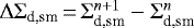 can be expressed as
 (14)
(14)
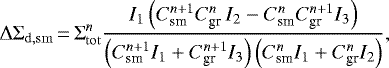
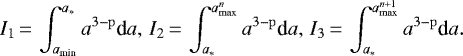
where  and
and  are the normalization constants for small and grown dust size distributions at the current (n) and next (n + 1) time steps, and the integrals
  ,
,  , and
, and  are defined as
 (15)
(15)
By introducing different normalization constants for small and grown dust we implicitly assume that the dust size distribution can be discontinuous at a*, which may develop due to different dynamics of small and grown dust. In this work, we suggest that dust growth due to the S term smooths out the discontinuity each time it could occur after the advection step. Physically this assumption corresponds to the dominant role of dust growth rather than dust flow in setting the shape of the dust size distribution. This can be achieved by setting  in Eq. (14). After determining the normalization constants
  and
and  from the known dust surface densities
  and
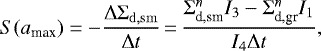
and  at the current time step, the rate of small-to-grown dust conversion during one time step Δt is then written as
 (16)
(16)
where the integral  is written as
 (17)
(17)
To complete the calculation of  , the maximum radius of grown dust amax in a given computational cell must be computed at each time step. The evolution of amax is described as
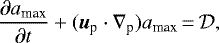 (18)
(18)
where the growth rate  accounts for the change in amax due to coagulation and the second term on the left-hand side account for the change of amax due to dustflow through the cell (the left-hand side is the full derivative of amax over time). We write the source term
  as
as
 (19)
(19)
where ρd is the total dust volume density and vrel is the dust-to-dust collision velocity. The adopted approach is similar to the monodisperse model of Stepinski & Valageas (1997) and is described in more detail in Vorobyov et al. (2018). The maximum value of amax is limited by the fragmentation barrier (Birnstiel et al. 2012) defined as
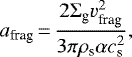 (20)
(20)
where vfrag is the fragmentation velocity set equal to a constant value of 3 m s−1 and cs is the speed of sound. Whenever amax exceeds afrag, the growth rate  is set to zero. We note that FEOSAD does not consider the Stokes regime of dust dynamics (which requires a different approach to calculating the friction force, see Stoyanovskaya et al. 2020) and the growth of dust is also limited to keep the size of dust particles within the Epstein regime. We also note that we do not take the possible dust sublimation at high temperatures into account and neglect dust diffusion associated with turbulence, which may affect the shape of dust rings discussed in Sect. 3.2. To summarize, our dust growth model allows us to determine the maximum size of dust grains and the dust-to gas mass ratio as a function of radial and azimuthal position in the disk, assuming that the slope p of the dust size distribution stays locally and globally constant.
2.3 Magnetic field calculations
In Eq. (2), the last two terms represent the magnetic tension force and the force due to the magnetic pressure gradient. We neglected a smaller term  that measures the planar force due to the pressure of the magnetic field at the surface pushing the disk when there is a planar gradient of its scale height, because a numerical instability of uncertain origin often develops when this term is taken into account.
2.3.1 The z-component of magnetic field
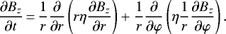
To calculate the vertical component of magnetic field  , we consider a simplified form of the induction equation taking Ohmic dissipation and magnetic ambipolar diffusion into account. The induction equation can be written in a general form as (see, for example, Dudorov 1995)
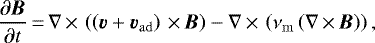 (21)
(21)
where  is the magnetic field, v is the gas velocity, vad is the velocity of ambipolar diffusion, and νm is the Ohmic diffusivity. Assuming steady magnetic ambipolar diffusion, we can write vad as
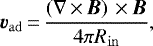 (22)
(22)
where 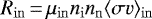 is the friction coefficient between ions and neutrals, μin is the reduced mass of ions and neutrals, ni is the number density of ions, nn is the number density of neutrals,
  is the “slowing-down” coefficient (Spitzer 1978). Ohmic diffusivity is calculated as
 (23)
(23)

is the electrical conductivity, e is the electron charge, ne is the number density of electrons, me is the mass of the electron, and νen is the mean collision rate between electrons and neutral particles, defined as
 (25)
(25)
where  (Nakano 1984) is the “slowing-down” coefficient for the electron-neutral collisions.
In the adopted thin-disk approximation, the magnetic field and gas velocity have the following nonzero components in the disk:  and
and  , respectively. The z-component of Eq. (21) can then be written as
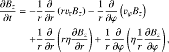 (26)
(26)
is the total magnetic diffusivity, and
 (28)
(28)
is the ambipolar diffusivity. The first two terms in the right-hand side of Eq. (26) are responsible for the advection of the z-component of magnetic field, while the last two terms describe the magnetic field diffusion.
To solve numerically Eq. (26), we use operator splitting in physical processes and split it into advection and diffusion equations:
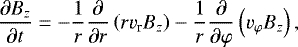 (29)
(29)
 (30)
(30)
Equation (29) is solved using the same third-order accurate piecewise-parabolic advection scheme (Colella & Woodward 1984) as for other hydrodynamic quantities (e.g., surface density, internal energy). Equation (30) is a nonlinear diffusion equation and its solution usually requires time-consuming implicit methods. We tried a fully implicit scheme and found that the simulations were decelerated by almost a factor of 10. Since in this work we aimed at studying the burst statistics over long evolutionary times (~1.0 Myr), we decided to adopt the ideal MHD limit and neglect the effect of Ohmic dissipation and ambipolar diffusion on  . We will return to the nonideal effects in a follow-up study focusing more on the characteristics of individual bursts.
2.3.2 The planar components of magnetic field
We calculate the planar components of magnetic field,  , by solving the same Poisson integral as for the gravitational field but with the source term
  replaced with
  . Here,
  is the strength of a uniform background vertical magnetic field. This approach can be justified as follows. The magnetic field in the region z ≥ 0 can be written as
  , where
  represents the background uniform magnetic field that is generated by distant currents, whereas
  is generated by currents contained within the disk. In the external medium to the disk, the current
  , hence we can write the magnetic field as the gradient of a scalar magnetic potential ΦM. Furthermore the divergence-free condition on
  means that ΦM (r, ϕ, z) can be determined by solving the Laplace equation ∇2ΦM = 0 for z ≥ 0. For simplicity, we use the magnetic potential method to calculate
  since
since  independently satisfies the curl-free and divergence-free conditions, and because
  as r, z →∞, in analogy with the gravitational field problem. The boundary condition at the disk upper surface is
  . Hence, the boundary value problem to determine the magnetic potential ΦM is formally identical to that for the gravitational potential Φ but with thesource term
  replaced by
  . Consequently
![\begin{align*} &\Phi_{\textrm{M}}(r,\phi,z\,{=}\,0)\\ \nonumber &\quad\ ={+}\frac{1}{2\pi} \int_{r_{\textrm{sc}}}^{r_{\textrm{out}}} r^{\prime} {\textrm{d}}r^{\prime} \int_0^{2\pi} \frac{[B_z^+(r^{\prime},\phi^{\prime})-B_0] \textrm{d}\phi^{\prime}} {\sqrt{{r^{\prime}}^2 + r^2 - 2 r r^{\prime} \cos(\phi^{\prime} - \phi) }},\end{align*}](/articles/aa/full_html/2020/12/aa39081-20/aa39081-20-eq105.png) (31)
(31)
and we can then determine  at the top surface of the sheet.
The gas that flows into the sink cell carries a magnetic flux with it. To estimate the magnitude of the r-component of magnetic field that is brought to the sink cell with this flow,  , we employ asimilar method as above. We first calculate the gravitational potential in the plane of the disk created by the matter that is accumulated in the sink cell:
![\begin{eqnarray*} \Phi_{\textrm{sink}}(r,\phi,z\,{=}\,0) &\,{=}\,& - {4 G M_{\textrm{sink}} \over \pi r_{\textrm{sc}}} \\ \nonumber &&{\times}\, \left[ K_2 {r \over r_{\textrm{sc}}} + K_1 \left({r_{\textrm{sc}} \over r} - {r \over r_{\textrm{sc}}} \right) \right], \end{eqnarray*}](/articles/aa/full_html/2020/12/aa39081-20/aa39081-20-eq108.png) (32)
(32)
where  is the total mass of gas and dust in the sink, and
  and
and  are the elliptic integrals of the first and second kind. The scalar magnetic potential of the sink cell is then calculated as
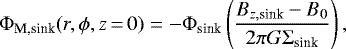 (33)
(33)
where  is the magnetic field in the sink cell and Σsink is the surface density of gas and dust in the sink cell determined from the boundary conditions (see Sect. 2.5). The planar component of magnetic field in the disk
  is then modified to take an additional input from the sink cell into account:
  .
.
2.3.3 Ionization fraction
Ohmic diffusivity (Eq. (23)) and ambipolar diffusivity (Eq. (28)) depend on the ionization fraction x = ne∕(ne + ni + nn), where we assume that electrons and ions are the only charge carriers. We calculate x following Dudorov & Sazonov (1987; see also Dudorov & Khaibrakhmanov 2014). Under conditions of low temperatures,  K, the ionization fraction is determined from the balance equation of collisional ionization, radiative recombination, and recombination on dust grains
 (34)
(34)
where ξ is the ionization rate,
 (35)
(35)
is the radiative recombination rate (Spitzer 1978).
We consider ionization by cosmic rays with a rate
 (36)
(36)
where Σcr = 100 g cm−2 is the attenuation depth of the cosmic rays. Additionally, the ionization by radionuclides is included, ξre = 7.6 × 10⁻¹⁹ s−1 (Umebayashi & Nakano 2009). The total ionization rate is ξ = ξcr + ξre.
In the regions where the gas temperature exceeds several hundred Kelvin, thermal ionization of alkali metals takes place. We evaluate thedegree of thermal ionization by considering ionization of potassium as a metal with lowest ionization potential (see Dudorov & Khaibrakhmanov 2014),
 (37)
(37)
where  is the cosmic abundance of potassium, set equal to 10−7 in this work. This value is added to the ionization fraction x determined from Eq. (34).
Our model has two populations of dust grains: small and grown ones. The total rate of recombination onto the dust grains is calculated as a sum of the rates for both populations,  . The rate of recombinations onto the dust grains of a given population is calculated as
 (38)
(38)
where  is the ratio of the dust volume number density nd to the gas volume number density ng in the disk midplane, σd = πa2 is the grain cross-section, vi is the thermal speed of ions with mass 30 mH, which is an approximate value that is representative of the dominant ionic species, for example, HCO+ and N2 H+. We note that
  is nonhomogeneous in our model and may change spatially and temporally as the dust grows and drifts inwards. Brackets ⟨… ⟩ denote averaging over the dust size distribution of a given dust population (small or grown). The gas and dust surface densities are turned into volume number densities in the disk midplane assuming a Gaussian distribution in the vertical direction. Small grains are considered to be well-mixed with gas and have the same scale height as the gas. The grown dust grains are prone to sedimentation, so that their scale height can differ from the scale height of the gas. In the present simulations, we neglect this difference and assume similar scale heights for grown dust and gas. The effect of different scale heights of gas and dust was explored in Vorobyov et al. (2018), who showed that the presence of dust settling has little effect on the size of dust grains in the inner disk where the grain size is limited by the fragmentation barrier, which does not depend on the dust volume density.
2.4 Adaptive turbulent viscosity and “dead” zones
Viscosity is an important mechanism of mass and angular momentum transport. A possible source of viscosity in protoplanetary disks is turbulence induced by the magnetorotational instability. In FEOSAD the turbulent viscosity is taken into account via the viscous stress tensor Π, the expression for which in the thin-disk limit can be found in Vorobyov & Basu (2010). We describe the magnitude of kinematic viscosity  using the α-parameterization of Shakura & Sunyaev (1973).
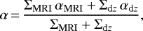
Unlike our previous studies of protoplanetary disks that assumed a spatially uniform and temporally constant α-parameter (e.g., Vorobyov et al. 2018), we employed in this paper an adaptive α-prescription based on the method presented in Bae et al. (2014). These authors introduced an adaptive α-parameter of the form
 (39)
(39)
where ΣMRI is the gas column density of the MRI-active layer at a given position in the disk, αMRI is the α-parameter in the active layer, Σdz is the gas column density of the MRI-inactive layer at the same position, and αd z is the α-parameter in the MRI-inactive layer. In this fashion, the adaptive α-parameter is calculated as a density-weighted average between an MRI-active value αMRI, usually taken to be 0.01, and an MRI-dead value αdz, usually taken to be in the 10−4–10−5 range. The spatial region characterized by a significantly reduced α-value is called the dead zone. In the method of Bae et al. (2014), the gas column density of the MRI-active layer of the disk is a fixed parameter, usually taken to be 100 g cm−2. If the gas surface density to the midplane of the disk is smaller than this value, the entire disk column is MRI-active. In this method, thetransition from the MRI-dead to MRI-active state can also occur if the gas temperature in the midplane exceeds a certain critical value for thermal ionization to set in, also usually taken to be a parameter in the 1000–1500 K range.
In this paper, we further upgraded this method with the purpose to reduce the number of free parameters that enter the adaptive α-prescription. More specifically, the dead zone is now defined as a disk region characterized by small ionization fraction and effective diffusion of magnetic field. In these disk regions, the MRI is not supposed to develop and, as a result, the MHD turbulence is weakened or absent. The boundary of the dead zone approximately coincides with the isosurface of the ionization fraction, at which the condition for suppressing the MRI is fulfilled (see Gammie 1996). Following Sano et al. (2000), we determine the boundary of the dead zone from the equality of the wavelength of the most unstable MRI mode, λMRI, and the gas scale height of the disk  . In the case of efficient magnetic diffusion, λMRI = 2πη∕va, where va is the Alfvén speed.
Following Bae et al. (2014), we set αdz = 10−5. Unlike these authors, however, we assume that αMRI is not constant throughout the disk. The peak value of α-parameter is higher in the disk regions directly involved in the burst than in otherwise MRI-active regions (e.g., outer disk with high ionization). This choice is motivated by numerical magnetohydrodynamics simulations of Zhu et al. (2020) suggesting that the α-value in the innermost disk regions during the MRI burst can exceed notably the typical value of 0.01 for MRI-active disks in the nonburst state (Yang et al. 2018).
The gas column densities of the MRI-active and MRI-dead zones ΣMRI and Σd z are calculated as follows. We substitute the expression for Ohmic diffusivity (Eq. (23)) together with formulae ((24)–(25)) for conductivity and collision rate with ne = xnn, as well as the Alfvén speed,  , with the critical gas volume density
  ) into the equality
  , and derive the critical gas surface density Σcrit for the MRI development as a function of
  , x, and
  ,
,
![\begin{equation*} \Sigma_{\textrm{crit}}\,{=}\,\left[\left(\frac{\pi}{2}\right)^{1/4}\frac{c^2m_{\textrm{e}}\langle\sigma v\rangle_{\textrm{en}}}{e^2}\right]^{-2}B_z^2 H_{\textrm{g}}^3 x^2.\end{equation*}](/articles/aa/full_html/2020/12/aa39081-20/aa39081-20-eq134.png) (40)
(40)
We note that Σcrit is derived using Ohmic diffusivity but neglecting other nonideal MHD effects. The reason for this is that Ohmic dissipation is known to prevail over ambipolar diffusion in the innermost several au of the disk (see, e.g., Balbus & Terquem 2001; Kunz & Balbus 2004), where the MRI-triggered bursts are localized. The Hall effect may also be important in these inner regions but its implementation in the thin-disk limit is not straightforward. The surface densities of the MRI-active and MRI-dead zones are then chosen according to the following algorithm:

If Σg ≥ Σcrit, a dead zone begins to develop at a given location in the disk. The depth of the dead zone in terms of the α-value is determined by the balance between ΣMRI and Σdz (see Eq. (39)). The analysis of Eq. (41) demonstrates that a sharp increase in Σcrit and hence the onset of the burst occurs if the ionization fraction x experiences a sharp rise. The  -component of magnetic field and the gas scale height
  are not expected to vary on short timescales in our model. We note that the inclusion of Ohmic dissipation (neglected in the current paper) in the magnetic induction equation may reduce the magnitude of
  in the inner disk, thus reducing Σcrit and increasing the radial extent of the dead zone. We note that Criterion (40) formally implies that there is no MRI if
  is zero. This state is, however, never realized in our global disk simulations because some nonzero
  component is always dragged in to the disk by the cloud core collapse. Although the development of MRI is possible in a purely toroidal field geometry, the
  component is known to enhance the instability (e.g., Hawley et al. 1995).
When compared to the method of Bae et al. (2014), ΣMRI in our model is no longer constant but is a spatially and temporally varying function of  ,
,  , and x. There is also no fixed temperature for thermal activation of the MRI; the MRI thermal activation now depends on the ionization fraction xth. A similar dependence of ΣMRI on the disk parameters was adopted in one-dimensional viscous disk models of Martin et al. (2012a).
2.5 Boundary conditions
The inner computational boundary cannot be placed at its physical distance from the protostar (usually much less than 0.1 au) because of strict limitations imposed by the Courant condition on the time step. Placing the inner boundary at several au and thus relaxing the Courant condition, as was done in our previous hydrodynamic collapse simulations (e.g., Vorobyov & Basu 2010),carries a risk of cutting out the disk regions that may be dynamically important for the entire disk evolution (see, e.g., Vorobyov et al. 2018). Here, the inner boundary of the computational domain was placed at rsc = 0.52 au, which is a reasonable compromise between computational time and physical realism, allowing us to capture the MRI triggering that occurs at sub-au scales.
Care should be taken when choosing the type of flow through the inner boundary. If the inner boundary allows for matter to flow only in one direction, namely, from the disk to the sink cell, then any wave-like motions near the inner boundary, such as those triggered by spiral density waves in the disk, would result in a disproportionate flow through the sink-disk interface. As a result, an artificial depression in the gas density near the inner boundary develops in the course of time because of the lack of compensating back flow from the sink to the disk.
To reduce the possible negative effect of the disproportionate flow, the FEOSAD code features the special inflow-outflow inner boundary condition at the sink cell-disk interface as described in Vorobyov et al. (2018) and Kadam et al. (2019). The mass of material that crosses the sink-disk interface is further redistributed between the central protostar and the sink cell as  according to the following algorithm (note that
  is always positive definite):
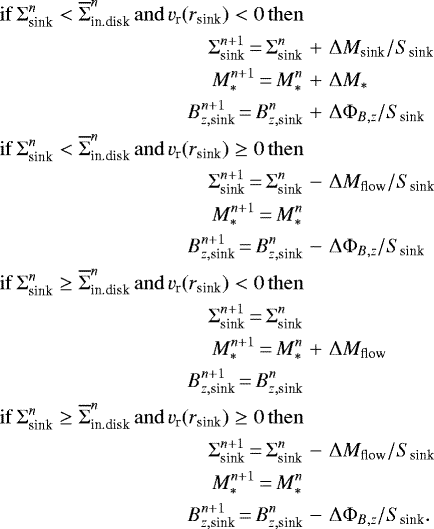
Here, Σsink is the surface density of gas (or dust) in the sink cell,  is the averaged surface density of gas (or dust) in the inner active disk (the averaging is usually done over one au immediately adjacent to the sink cell),
  is the surface area of the sink cell, and vr(rsink) is the radial component of velocity at the sink–disk interface. We note that vr (rsink) < 0 when the gas flows from the active disk to the sink cell and vr(rsink) > 0 in the opposite case. The superscripts n and n + 1 denote the current and the updated (next time step) quantities. The exact partition between
  and
and  is usually set to 95%:5%. This means that most of the matter that crosses the sink–disk interface quickly lands on the star, implying a fast mass transport through the sink cell which can be expected in the MRI-active limit.
The flow of matter to and from the sink cell carries magnetic flux with it. Therefore, the inner boundary condition also modifies the z-component of magnetic field in the sink cell  based on the amount of magnetic flux
  that is carried in or out of the sink cell with the flow of matter. Our inner boundary is designed so that an initially spatially constant mass-to-flux ratio λ stays constant both in the entire computational domain and in the sink cell during disk evolution in the ideal MHD limit. The fact that λ stays constant in the ideal MHD limit serves as an assuring test on our numerical scheme and boundary conditions. Of course, when the nonideal MHD effects are considered, the mass-to-flux ratio may become nonhomogeneous. We note that the constant λ condition implies that most of the initial magnetic flux is advected with the gas flow to the sink cell by the end of numerical simulations. If this flux is further brought to the star, then the magnetic field of the star would become much greater than what is measured even for the most magnetized T Tauri stars, signifying the importance of nonideal MHD effects in redistributing the magnetic flux in the star and disk formation process.
The calculated surface density and z-component of magnetic field in the sink cell  and
and  are used at the next time step as the inner boundary values for Σg, Σd,gr, Σd,sm, and
  . The radial velocity and internal energy at the inner boundary are determined from the zero gradient condition, while the azimuthal velocity is extrapolated from the active disk to the sink cell assuming a Keplerian rotation. We ensure that our boundary conditions conserve the total mass and magnetic flux budget in the system. Finally, we note that the outer boundary condition is set to a standard free outflow, allowing for material to flow out of the computational domain, but not allowing any material to flow in.
Model parameters.
2.6 Initial conditions
The initial radial profile of the gas surface density Σg and angular velocity Ω of the pre-stellar core has the following form:
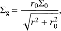 (43)
(43)
![\begin{equation*} \Omega\,{=}\,2\Omega_{0}\left(\frac{r_{0}}{r}\right)^{2}\left[\sqrt{1+\left(\frac{r}{r_{0}}\right)^{2}}-1\right],\end{equation*}](/articles/aa/full_html/2020/12/aa39081-20/aa39081-20-eq157.png) (44)
(44)
where Σ0 and Ω0 are the angular velocity and gas surface density at the center of the core, 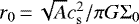 is the radius of the central plateau, where cs is the initialsound speed in the core. This radial profile is typical of pre-stellar cores with a supercritical mass-to-flux ratio that are formed through ambipolar diffusion, with the specific angular momentum remaining constant during axially-symmetric core collapse (Basu 1997). The value of the positive density perturbation A is set to 2.0, making the core unstable to collapse. Initially all dust is in the form of small sub-micron dust grains. The surface density and angularvelocity profiles of small dust follow that of gas with the initial dust-to-gas mass ratio set equal to 1:100.
The initial gas temperature in collapsing cores is  . We consider several initial cloud cores, the parameters of which are listed in Table 1. The initial spatially uniform mass to flux ratio
  is given in units of the critical value
  . The initial distribution of magnetic field
  is determined from λ. The strength of a uniform background vertical magnetic field
  is set to 10−5 G.
2.7 Solution procedure
Equations (1)–(3) and (11)–(13) are solved in polar coordinates (r, ϕ) on a numerical grid with 256 × 256 grid zones. The radial points are logarithmically spaced. The innermost grid point is located at the position of the sink cell rsc = 0.52 au, and the sizeof the first adjacent cell is about 0.018 au (it may vary slightly depending on the model). The sub-au resolution isthus achieved in the inner 30 au regions of the disk. We use a combination of finite-differences and finite-volume methods with a time-explicit solution procedure similar in methodology to the ZEUS code (Stone & Norman 1992a). The advection is treated using the third-order-accurate piecewise-parabolic interpolation scheme of Colella & Woodward (1984). The update of the internal energy per surface area due to cooling Λ and heating Γ is done implicitly using the Newton-Raphson method of root finding, complemented by the bisection method where the Newton–Raphson iterations fail to converge. The accuracy is guaranteed by not allowing the internal energy to change more than 15% over one time step. If this condition is violated in a particular cell, we employ subcycling for this cell, namely, the solution is sought with a local time step that is smaller than the global time step by a factor of 2. The local time step may be further decreased until the desired accuracy is reached.
The terms describing turbulent viscosity are implemented in the code using an explicit finite-difference scheme. This is found to be adequate for α ≤ 0.01 because other terms (usually, the azimuthal advection) dominate in the Courant condition that controls the time step, even though we use the FARGO algorithm to accelerate calculations in Keplerian disks (Masset 2000). A small amount of artificial viscosity is added to the code to smooth out shocks over two grid zones. The associated artificial viscosity torques integrated over the disk area are negligible in comparison with gravitational or turbulent viscous torques. Finally, the Courant time-step condition was modified to include the limiters due to the magnetic field, following Stone & Norman (1992b). The adopted Courant number is 0.5. The dust friction term fp between gas and dust (including backreaction of dust on gas) is calculated using the fully implicit algorithm presented in Stoyanovskaya et al. (2018). The standard test problems (Sod shock tube and dusty wave) have demonstrated a clear superiority of this method over semi-implicit schemes.
3 Global disk evolution with magnetic field
In this section, we consider the global evolution of the disk in the thin-disk limit in the presence of a magnetic field. We choose model 2 as a fiducial model for this purpose.
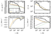 |
Fig. 1 Azimuthally averaged radial profiles of the gas surface density (panel a), temperature (panel b), gas radial (panel c) and azimuthal velocities (panel d) at different evolution times after the onset of the simulation (1: 0 kyr, 2: 54.9 kyr, 3: 55.1 kyr, 4: 56.0 kyr, 5: 56.2 kyr, 6: 156.2 kyr). The black dashed lines with labels show typical slopes. |
3.1 Initial stages of collapse and disk evolution
Firstly, we discuss the process of disk formation. In Fig. 1, we plot the averaged radial profiles of gas surface density ⟨Σg ⟩, gas midplane temperature  , radial and azimuthal velocities of gas ⟨vr⟩ and ⟨vϕ⟩ at different evolution times. Initially, the prestellar core has a uniform, rigidly rotating plateau in the center with ⟨Σg ⟩ = 0.62 g cm−2. In the outer parts, the surface density declines as r−1, while the azimuthal velocity becomes nearly constant. The gas temperature is 20 K throughout the core. By the time t = 54.9 kyr (gray solid lines), the surface density grows by a factor of 20 in the central part of the core. At r > 100 au, the surface density profile obeys a nearly self-similar law ⟨Σg⟩∝ r−1, except for the regions near the outer boundary where a rarefaction wave develops and the surface density drops faster than ⟨Σg ⟩∝ r−1 (Vorobyov & Basu 2005b). The gas temperature remains close to the initial value 20 K at this time. The radial velocity profile becomes nonmonotonic: a maximum infall rate of ⟨vr ⟩ ~ 0.02 km s−1 is reached in the outer part of the cloud, r ≈ 200 au. The rotation profile remains nearly rigid at r < 50 au, while differential rotation with ⟨vϕ ⟩≈ 3 × 10⁻² km s−1 establishes in the outer regions.
At t = 55.5 kyr after the start of the collapse (orange dashed lines), the surface density grows by two orders of magnitude and the temperature increases by factor of 10 in the central part of the core. The infall velocity ⟨vr ⟩ monotonically increases from nearly zero at the outer boundary of the computational domain to − 0.4 km s−1 at the innerboundary. At this time instance, differential rotation establishes in the entire cloud with ⟨vϕ ⟩ being a decreasing function of radius. It should be noted that the gravitational field of the system is initially determined only by the mass of the infalling gas.
At t ≈ 55.5 kyr, the mass of gas in the sink cell exceeded 0.02  . We further assume that the phenomenon known as the second collapse, due to molecular hydrogen dissociation, has occurred in the sink cell, leading to the formation a protostar. Therefore, we place a point-like gravity source at the coordinate origin. The formation of the central star changes the gravitational field of the system, so that the gas in the inner regions starts falling faster toward the star. As a result, the gas surface density decreases at t = 56 kyr (black dotted line) compared to the previous evolution times. The slope of the surface density profile is no longer self-similar. The temperature of the gas grows to≈600 K near the inner edge of the computational domain thanks to stellar illumination and compressional heating. The radial profile of ⟨vr ⟩ becomes nonmonotonic: gas in the outer regions falls with increasing velocity, while the gas in the innermost regions decelerates when approaching the star, ushering the formation of a centrifugally balanced disk. A maximum infall velocity ≈ − 0.4 km s−1 is reached at r ≈ 1 au. The deceleration of the gas in the innermost region, r < 1 au, is caused bythe action of the centrifugal force. According to Figs. 1c and 1d, the azimuthal velocity of the gas becomes greater than the radial velocity in this region, namely, the centrifugal barrier forms.
Shortly after the formation of the central protostar, at t ≈ 56.4 kyr (the gray dashed lines in Fig. 1), a bump in the gas surface density appears at r < 5 au. As Fig. 1c demonstrates, the radial velocity of the gas approaches zero inside this region. This bump corresponds to the newly formed disk, which is the region where the centrifugal force hinders the further infall of the gas from the envelope. In the subsequent evolution, the disk grows due to the continual mass-loading from the infalling envelope.
Mass-loading from the envelope and transport of mass due to viscous torques (they can be positive in the disk outer regions) lead to the disk spreading with time, as is evident from the black solid lines in Fig. 1. A peak in the gas surface density develops at several au, while the outer parts are characterized by a power-law density profile, ⟨Σg ⟩∝ r−1.5. The temperature decreases from ≃700 K at r = 1 au to 20 K at r > 1000 au. The slope of the temperatureprofile is nearly − 0.5 in the region r < 10 au. Both density and temperature profiles exhibit a nonmonotonic behavior in the region r < 20 au: there are variations of the surface density with amplitude of ~1000−5000 g cm−2 and temperature variations with amplitudes of ~100−300 K on spatial scales of ~1 au. These variations lead to the development of local pressure maxima and to the formation of dust rings discussed later in Sect. 3.2. The dynamics of the disk is characterized by a slowly variable radial transport with ⟨vr ⟩≤ 0.01 km s−1 within the disk, r < 200 au, and fast infall onto the outer edge of the disk with velocity ⟨vr⟩ ~ −0.1 km s−1. The radial profile of azimuthal velocity follows a power-law dependence ⟨vφ ⟩∝ r−0.45 at r < 100 au, namely, the disk is slightly super-Keplerian. The ⟨vφ⟩ radial profile is super-Keplerian due to the contribution of disk self-gravity to the gravity of the central protostar.
3.2 Long-term disk evolution
In Fig. 2, we plot the spatial distributions of the gas surface density in the 600 × 600 au2 box at different time instances after disk formation. The disk forms at t ≈ 0.056 Myr after the onset of the collapse and its subsequent evolution can be divided into two phases. In the first phase, t < 0.2 Myr, the disk grows with time due to viscous spreading and continual mass-loading from the envelope. To illustrate the disk growth with time, we adopt Σ = 1 g cm−2 as a typical surface density at the outer boundary of the disk. Figure 2 shows that the disk quickly grows up to a typical size of 100–150 au by the time t = 0.2 Myr. Spiral arms form at this time period, which reflect the development of gravitational instability in the disk. In the second phase, t > 0.2 Myr, the disk radius only slowly increases with time. No spiral arms are observed in this phase. Instead, ring structures form in the innermost region of the disk at r ≤ 15−20 au. These rings with a gas surface density of ≳200 g cm−2 persist till the end of the simulation. Similar ring-like structures were also reported in numerical hydrodynamics simulations of disk formation with an adaptive α by Kadam et al. (2019).
These gas rings also represent the local pressure maxima, which help collecting grown dust into similar ring-like structure but of much higher contrast. Figure 3 presents the spatial distribution of grown dust surface density in the inner 60 × 60 au2 box at the same evolutionary times as in Fig. 2. A series of concentric dust rings is formed in the inner ten astronomical units. The localization of the rings coincides with the radial extent of the dead zone, as will be shown later in Fig. 7. We note that turbulent dust diffusion (neglected in this study) may smooth out the dust rings obtained in our study, but low α-values in the rings could require Schmidt numbers ≪1.0 for this effect to be pronounced. Interestingly, the rings evolve with the disk, their radial position and shape change with time. The total dust to gas mass ratio in the rings can reach 0.1, while in the rest of the disk it is reduced below the initial 1:100 value. The concentration of dust in the dead zones was also predicted in previous studies of protoplanetary disks (e.g., Dzyurkevich et al. 2014; Vorobyov et al. 2018; Kadam et al. 2019). Variations in the gas pressure and its radial gradient within the dead zone extent may be responsible for the formation of a series of dust rings in our models. Strong concentration of grown dust in the rings may be offset by including addition physics, such as turbulent diffusion or dependence of dust sticking properties on presence or absence of ices, which would also affect the level of dust backreaction on gas. We postpone a more detailed analysis of the ring formation mechanisms, ring properties, and other implications of the dead zone (e.g., the Rossby wave instability) to a follow up study.
Figure 4 presents the azimuthally averaged profiles of several quantities that describe in more detail the dust distribution in the disk. Two time instances corresponding to the bottom-left and bottom-right panels of Fig. 2 are shown. The top row presents the surface densities of small and grown dust (Σd,sm and Σd,gr, respectively) and also the vertically integrated gas pressure  , while the bottom row shows the dust maximum radius amax, Stokes number St = Ωtst, and total dust-to-gas mass ratio d2g = (Σd,sm + Σd,gr)∕Σg. Here, Ω is the local angular velocity and tst is the stopping time. We note that we use the Keplerian angular velocity as a proxy for Ω. This could underestimate the Stokes number because the disk gravity makes the disk rotate faster than what is expected from the pure Keplerian rotation.
Several interesting features can be noted in the dust distribution. First, grown dust dominates over small dust in the bulk of the disk, except for the outer regions beyond 100 au. To remind the reader, all dust was initially in the form of small dust grains whenthe gravitational collapse commenced. The efficient conversion of small to grown dust is the result of dust growth, as can be seen from the black line in the bottom row. The maximum dust radius reaches 5.0 cm at t = 0.199 Myr and 10 cm at t = 0.549 Myr. The most efficient dust growth occurs in the inner 10 au where the dead zone is localized. Beyond the dead zone, amax does not exceed a few ×10−2 cm. Second, the local peaks in the dust density coincide with the local pressure maxima, corroborating our previous suggestions about dust drift. Third, the dust-to-gas ratio is generally below 1:100, which was the initial value for the prestellar core. The exception are the most pronounced dust rings where d2g can exceed 1:100 and reach 1:10 in the late disk evolution. The general decrease of d2g throughout the disk is likely due to dust loss to the star during accretion bursts. Dust accumulates in the dead zone and is dumped on the star during bursts in higher amounts than would be expected without accumulation. We checked the dust-to-gas mass ratio in the star and it is indeed slightly elevated 0.012. Finally, the Stokes number is relatively low, hardly exceeding 10−1 within 100 au. A sharp increase of St beyond 100 au is the result of a sharp increase in tst in the rarefied outer regions. Our simulations show that a Stokes number on the order of unity, sometimes taken to be representative for protoplanetary disks (e.g., Booth & Ckarke 2016), may be an overestimate.
In Fig. 5, we plot the space-time diagrams of the azimuthally averaged surface density profiles for gas, ⟨Σg ⟩, and grown dust,  . Firstly, we consider the gas surface density distribution shown in the left panel. The white contour line showing the locus of ⟨Σg ⟩ = 1.0 g cm−2 indicates that the disk quickly grows in time in the initial formation stage and reaches a radius of approximately 200 au by the end of the simulations. Moreover, ⟨Σg⟩ is highest in the inner several tens of astronomical units, but its radial distribution is not monotonic. Several rings of enhanced gas density appear in this region after 0.2 Myr and persist till the end of the simulations. The farthest ring is located at 15 au from the star. We emphasize the horizontal stripes that are evident in the left panel. These structures reflect MRI-triggered bursts that will be discussed in more detail in Sect. 4. The grown dust distribution shown in the right panel is more patchy. It also shows rings, but of higher contrast than those of the gas, reflecting efficient dust drift to the local pressure maxima (see also Fig. 3). The grown dust distribution is also characterized by horizontal stripes akin to those seen in the left panel, but of higher contrast.
In Fig. 6, we plot the space-time diagrams of the azimuthally averaged temperature and magnetic field profiles. The temperature inside the disk reaches values above 103 K in the inner several astronomical units. Horizontal stripes akin to those of the gas and dust density distributions are also evident in the gas temperature distribution. Overall, the disk cools as it evolves. The distribution of  follows that of the gas surface density distribution, as
  in the ideal MHD limit.
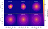 |
Fig. 2 Two-dimensional distribution of the gas surface density in inner 600 × 600 au2 box at time instances 0.049, 0.099, 0.149, 0.199, 0.349, 0.549 Myr after disk formation. White contours mark the disk loci with Σ = 1 g cm−2. The time is counted from the disk formation instance (t = 0.056 Myr). |
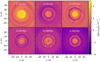 |
Fig. 3 Two-dimensional distribution of the grown dust surface density in the inner 6 × 60 au2 box at time instances 0.049, 0.099, 0.149, 0.199, 0.349, 0.549 Myr after disk formation. The time is counted from the disk formation instance. |
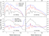 |
Fig. 4 Azimuthally averaged dust characteristics at t = 0.199 Myr (left column) and t = 0.549 Myr (right column) from the instance of disk formation. Top row: presents the surface densities of small and grown dust and also the vertically integrated gas pressure. Bottom row: shows the dust radius, Stokes number, and total dust-to-gas ratio. |
4 MRI-triggered accretion bursts
In this section, we analyze the temporal evolution of the rate of gas mass transport through the sink cell, Ṁg= −2πrscΣgvr. We use this quantity as a proxy for the mass accretion rate on the star. In Fig. 7a, we plot the time dependence of Ṁ starting from the disk formation instance till 0.7 Myr. The accretion rate is a few  right after disk formation and in general decreases afterwards. This trend is accompanied by short-time variability, during which the accretion rate rapidly increases by 1–3 orders of magnitude. The time scale of variability is initially very short, so that
  appears as a black strip in Fig. 7a at t < 0.1 Myr. The amplitude of variability is initially limited by one order of magnitude, but quickly increases to 2–3 orders of magnitude (see also Fig. 10). In this early stage, the inner disk is sufficiently hot to support thermal ionization of alkaline metals and the diskis mostly in the MRI-active state.
As the evolution continues and the inner disk cools, individual bursts of higher amplitude emerge as spikes in the  dependence after t = 0.1 Myr. Six accretion bursts occur in a time interval from 0.2 Myr after disk formation till 0.7 Myr. Figure 7b shows part of the Ṁ (t) dependence for a time interval from 0.149 to 0.150 Myr. One accretion burst is observed in this period. It has a sharp rise, typical for many classical FUors (e.g., FU Orionis and V1057),followed by a slow decline, and a sharp fall off after about 200 yr from the onset of the burst to a negligible value (implying that the matter stopped flowing toward the star for a short while). A small scale variability is evident during the outburst phase, which is also observed in some FUors (Kóspál et al. 2020). We defer a more detailed analysis of the burst statistics (peak luminosities, durations, rise times) to a follow-up paper.
To analyze the nature of the bursts, we plot the space-time diagram of the azimuthally-averaged ionization fraction ⟨x⟩ in Fig. 7c. We also depicted the boundary of the dead zone with the white contour line in this plot. The dead zone is determined as the disk regions where Σg < Σcrit and the boundary of the dead zone is located at the disk loci where Σg = Σcrit (see Eq. (40)). The orange rectangles in all panels and the inset in Fig. 7c highlight the accretion burst occurring at t ≈ 0.1493 Myr after the disk formation. Figure 7c shows that the ionization fraction is generally an increasing function of radius everywhere in the disk, except the innermost region. The smallest values of x ~ 10−17−10−16 are observed in the region from 1 to 10 au. Comparison of Figs. 5 and 7c reveals that the ionization fraction is lowest in the regions with highest gas and grown dust surface densities. This is because the rate of recombination onto the dust grains increases with gas density. Moreover, the ionization rate by cosmic rays decreases with increasing gas density due to cosmic ray attenuation.
The region of lowest ionization fraction is typically determined as a dead zone if x ≲ 10−13−10−12 (see, e.g., Sano et al. 2000; Dudorov & Khaibrakhmanov 2014). In the considered case, the outer boundary of the dead zone lies at r ≈ 15−20 au, just outside the dust rings in Fig. 3. Its position does not change appreciably during the disk evolution, except for the very early stages of disk formation. On the contrary, the location of the inner boundary of the dead zone is highly variable, mirroring the accretion variability in Fig. 7a. For instance, white stripes in Fig. 7c at t < 0.1 Myr appear because the inner boundary of the dead zone frequently moves from 0.4 au (inner boundary of the disk) to r ≈ 3−5 au and back, reflecting similar high-frequency variations in  . The horizontal white stripes in ⟨x⟩ become less frequent with time and so do the mass accretion bursts in the top-left panel. These white stripes encompass time instances when the disk region at r < 5 au becomes MRI-active and then MRI-dead again. The inset in Fig. 7c shows such an event occurred at a time interval from 0.149 Myr to 0.150 Myr. The lifetime of this MRI-active region is on the order of 200 yr.
Figure 7 suggests that the accretion bursts occur when the inner region of the disk, r < 5 au, becomes MRI-active. We refer to these events in the following text as the MRI-triggered bursts. To clearly demonstrate the causal link between the bursts, on the one hand, and ionization fraction, α-value and gas temperature, on the other hand, we plot the Ṁg dependence in the upper panel of Fig. 8 for a time interval from 0.149 to 0.150 Myr. Blue circles labeled as A, B, and C mark the pre-burst, mid-burst, and post-burst stages, respectively. Additionally, the two-dimensional spatial distributions of the ionization fraction (first row), α-value (second row), and gas temperature (third row) at time instances corresponding to stages A, B, and C are plotted in the right panel of Fig. 8. White contours in the two-dimensional panels delineate the dead zone boundary. We note that the inner boundary of the dead zone often coincides with the disk inner edge and is hence not visible in these plots.
Figure 8 shows that the ionization fraction is lowest (≈ 10−14) near the inner disk boundary and the dead zone extends to r ≈ 20 au in the pre-burst stage A. We note that the dead zone is not continuous and may be patchy, reflecting the ring-like structure of the inner disk. The ionization fraction is on the order of 10−13 at the boundary of the dead zone. The α-value in the dead zone is lower than 0.01 and the gas temperature does not exceed a few hundred Kelvin. At t = 0.1493 Myr (state B), the ionization fraction becomes higher, x ~ 10−8−10−7, in the innermost region of the disk, r < 5 au. The α-value and gas temperature also jump to 0.1 and >1000 K, respectively. This region becomes MRI-active, which leads to an enhanced accretion rate. After accretion burst, the active region at r < 5 au disappears and the accretion rate falls down to a pre-burst value (stage C). The α-value, and ionization fraction return to their pre-burst values, while the inner disk gradually cools down to the pre-burst state.
To further analyze the burst mechanism, we plot in Fig. 9 the time evolution of several quantities at the sink–disk interface (0.52 au) as the burst emerges and decays. In particular, the top row shows the mass accretion rate Ṁg and total luminosity  , while the other panels show the midplane temperature
  , gas and grown dust surface densities Σg and Σd,gr, α-parameter, and ionization fraction x at the sink-disk interface (0.52 au). The pre- and post-burst total stellar luminosity is about 3
  and the peak luminosity reaches 165
  . Small-scale variability during the active phase and also some moderate after-burst variability is also present. The midplane temperature before the burst is 650–700 K and the ionization fraction is below 10−13. However,
  rises gradually due to heating provided by residual viscosity with α = 10−5 and adiabatic compression provided by inflowing matter and spiral arms (Bae et al. 2014) until thermal collisions begin to ionize alkaline metals. This is a runaway process that depends exponentially on the temperature (see Eq. (37)). The rise in ionization is accompanied by the rise in viscous heating (via increased α), causing temperature to increase further and finally causing the burst. We note that the concentration of dust in the dead zone assists the process of MRI triggering because the increased optical depth makes the dead zone easier to warm up. We warn, however, that we use dust opacities that do not depend on dust growth (Semenov et al. 2003)and more accurate computations with dust-growth-dependent opacities are needed to confirm the effect.
At the onset of the burst  jumps sharply to 1800 K, but quickly declines below the pre-burst value as the burst develops and decays. The sharp rise in the midplane temperature is caused by strong viscous heating when the dead zone turns into an MRI-active region with a high α-value and drop in
  is caused by radiative cooling as the inner disk losses mass and becomes less optically thick to its own thermal radiation. The surface densities of gas and grown dust also drop during the burst, reflecting the loss of disk mass during the burst. We note that the drop in Σd,gr is deeper than in Σg, which can be explained by efficient accumulation and drift of grown dust in the dead zone prior the burst. As is expected, the α-value increases sharply during the burst and drops back to the pre-burst value when the burst is over. The same is true for the ionization fraction. It is worth noticing that both the mass accretion rate and total luminosity return to almost pre-burst values earlier than the burst is formally over, as is signalized by the drop of α and x to the pre-burst state.
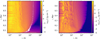 |
Fig. 5 Space-time diagrams of the azimuthally averaged radial profiles for the gas and grown dust surface densities (left and right panels, respectively). The white contour line indicates the disk loci with Σg = 1.0 g cm−2. |
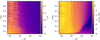 |
Fig. 6 Space-time diagrams of the azimuthally averaged radial profiles of temperature and
|

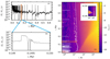 |
Fig. 7 Top left (a): the accretion rate onto the star versus time starting from disk formation. Bottom left (b): similar to the top-left panel, but for a time interval t = [0.149, 0.150] Myr. Orange rectangles mark the burst analyzed in Fig. 8. Right (c): space–time diagram of the azimuthally averaged ionization fraction. The white contour line delineates the dead zone boundary. The time is counted from the instance of disk formation. |
5 Parameter space study
Unlike many previous studies of the burst phenomenon, we can consider the effects of different initial conditions in pre-stellar cores on the development of MRI-triggered bursts in protoplanetary disks. Here, we vary the initial pre-stellar core mass and strength of magnetic field. Figure 10 presents the resulting mass accretion rates in four models, the parameters of which are listed in Table 1. More specifically, models 1, 2, and 3 have progressively smaller masses of the pre-stellar core ( ), while model 2L is characterized by an increased mass-to-flux ratio λ. The black lines show the mass accretion rate from the disk through the sink cell and the red lines correspond to the mass infall rate from the envelope onto the disk. The latter quantity is calculated as the mass flux at a radial distance of 1000 au from the star, except for model 3, in which case the infall rate is calculated at 400 au (this model is characterized by a compact initial core).
The accretion rate histories are different in models with distinct pre-stellar core masses. The higher mass models with  and 0.83
  (first and second panels) exhibit multiple bursts throughout the entire considered period of evolution (1.0 Myr). In particular, Ṁg in the early evolution is highly variable and the system spends roughly equal time in states of low- and high-rate accretion. The amplitude of variability spans one-to-two orders of magnitude. After about 0.08–0.1 Myr the accretion rate begins to clearly exhibit individual bursts interspersed with longer periods of low-rate quiescent accretion. This qualitative change in the behavior of protostellar accretion coincides with the time when the envelope infall rate begins to decline, reflecting the gradual depletion of the envelope material via infall on the disk. The frequency of the bursts further reduces with declining mass infall rate.
The apparent correlation of the burst activity with the disk mass-loading can be explained by the action of gravitational instability, which is strongest in the embedded phase thanks to mass-loading from the envelope that replenishes the disk mass lost via accretion onto the star. The associated gravitational torques are usually stronger than the viscous torques in the embedded phase (Vorobyov & Basu 2009), so that the both torques are very efficient in supplying the inner disk with matter and recharging the inner disk for the MRI-bursts to occur. When the envelope depletes, the gravitational instability diminishes and only the viscous torques remain operational, resulting in longer recharge times and longer quiescent periods. A similar phenomenon was described in Zhu et al. (2009a).
The lower mass model with  and the terminal stellar mass
  (fourth panel) demonstrates a different behavior. Accretion bursts occur only occasionally and are of much smaller amplitude than in the higher mass models. The mass accretion rate gradually declines with time to a small value of
  yr−1 by the end of the simulation, although order-of-magnitude variations can still be present at late evolutionary times. The mass infall rate declines much faster in this model, meaning that the embedded phase in this model is short-lived, less than 0.1 Myr.
Model 2L with an increased mass-to-flux ratio, but other characteristic similar to model 2, forms the disk notably earlier due to faster collapse of a less-magnetized core. The early disk evolution is characterized by a highly variable accretion and well defined bursts start occurring 50 kyr after the onset of collapse. The number and frequency of the bursts are not strongly affected by an increase of the mass-to-flux ratio by a factor of 5.
To understand the difference in the burst behavior between the considered models, we plot in Fig. 11 the space-time diagrams showing the time evolution of the azimuthally averaged ionization fraction ⟨×⟩ in model 2L (left) and model 3 (right). A comparison with the right panel of Fig. 7 showing the corresponding quantity for model 2 reveals that the dead zone has a different extent in the three models considered. It is largest in model 2L, with the outer boundary reaching 30 au in the early stages, and is smallest in model 3, extending only to 6–8 au. Consider first model 2L with an increased mass-to-flux ratio and reduced magnetic field. Eq. (40) indicates that reducing  also lowers the value of Σcrit (in the limit of Σcrit → 0 the entire disk is MRI-dead) and broadens the dead zone. This trend is somewhat offset by a mild increase in the ionization fraction. This occurs because the model with reduced magnetic field forms a more massive and warmer disk(strong magnetic fields delay the disk formation, spreading its evolution over a longer time). The net effect is a mild broadening of the dead zone in model 2L as compared to model 2 with stronger magnetic support.
In the case of model 3, the dead zone shrinks because the column density of gas decreases. This model has a much smaller reservoir of mass in the collapsing core and forms a disk of notably lower mass,  , in contrast to
  in model 2. Both values are referred to the end of simulations. The disk densities and temperatures are appreciably lower in model 3 and the thermal ionization of alkaline metals occurs only in the very early stages of disk evolution, when it is still relatively dense and warm thanks to mass-loading from the infalling envelope. To summarize, it appears that there exists a minimal mass of prestellar cores and stellar masses, below which the MRI-bursts in subsequently formed disks are unlikely to occur. A similar conclusion was made in Kadam et al. (2020). We checked if models 1, 2, and 2L may have bursts when the stellar mass is below
  (but grow later due to accretion). It turned out that when the clear-cut individual bursts start to occur (skipping the initial highly variable stage it is 0.11 Myr for model 1, 0.08 Myr for model 2, and 0.04 Myr for model 2L) the stellar mass is already above 0.25–0.3
  . Reducing the strength of magnetic field by a factor of 5 does not seem to have a notable effect on the frequency of accretion bursts. Finally, we note that our model does not reproduce the EX Lupi-like luminosity outbursts, which are known to occur in the Class II–III stages of disk evolution, most likely because these outbursts are caused by phenomena that operates much closer to the star than we can resolve in our global disk simulations (D’Angelo & Spruit 2012; Armitage 2016).
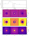 |
Fig. 8 Upper panel: accretion rate onto the star versus time in the time interval t = [0.149, 0.150] Myr after the disk formation. Lower rows of panels: two-dimensional distributions of the ionization fraction (first row), turbulent parameter α (second row), and gas temperature (third row) in the region r ≤ 30 au at time instants t = 0.1491, 0.1493 and 0.1497 Myr marked with blue rounds with labels “A”, “B” and “C” in the upper panel, respectively. The white contour delineates the boundary of the dead zone. |
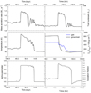 |
Fig. 9 Time evolution of several disk and burst characteristics at the sink–disk interface as the burst develops and decays. Shown are the mass accretion rate (top-left), total luminosity (top-right), midplane temperature (middle-left), gas and grown dust surface densities (middle-right), α-value (bottom-left), and ionization fraction (bottom-right). |
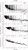 |
Fig. 10 Protostellar accretion rates (black lines) and envelope infall rates (red lines) as a function of time in models with various initial pre-stellar come masses and mass-to-flux ratios: model 1 –
|


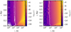 |
Fig. 11 Space-time diagrams showing the ionization fraction in model 2L (left) and model 3 (right). The white contour lines delineate the position of the dead zone. |
6 Comparison with previous studies and model caveats
The MRI-triggered accretion bursts were studied in detail in a series of papers (e.g., Armitage et al. 2001; Zhu et al. 2009a,b; Martin et al. 2012b), but here we focus on two most relevant studies by Bae et al. (2014) and Kadam et al. (2020). Both studies employ numerical hydrodynamics simulations in the thin-disk limit and use an adaptive α-parameter method to simulate the MRI bursts. The thermal physics is also similar, although Bae et al. (2014) used a more sophisticated two-temperature description of the disk vertical structure. The latter authors considered the effect of disk mass-loading from the envelope in a parametric manner, while Kadam et al. (2020) and we use a global model that computes the dynamics of both the disk and envelope in one simulation and on one numerical grid. The inner computational boundary in Bae et al. (2014) and Kadam et al. (2020) was set at 0.2 and 0.41 au, respectively, while in our study it is set equal to 0.52 au. A larger inner boundary in our study and in Kadam et al. (2020) is dictated by a heavier numerical load on a finer numerical resolution (256 × 256 or 512 × 512) in contrast to 128 × 128 in Bae et al. (2014).
The main difference of our work from aforementioned studies is that we take magnetic fields explicitly into account (albeit in a simplified flux-freezing approximation), evolve dynamically both the gas and dust disk subsystems, and also calculate explicitly the ionization fraction. This allowed us to reduce the number of free parameters when calculating the adaptive α-parameter (see Eq. (39)). For instance, Bae et al. (2014) and Kadam et al. (2020) used a critical temperature for MRI activation,  , set equal to 1300 to 1500 K. In our study this parameter is absent and the MRI activation depends on the explicitly calculated ionization fraction. Furthermore, Bae et al. (2014) and Kadam et al. (2020) used a fixed value for the MRI-active disk layer, ΣMRI, set equal to 10 or 100 g cm−2. In our approach, ΣMRI is a time- and space-varying quantity calculated from the strength of magnetic field and ionization fraction (see Eq. (40)).
Our simulations can reproduce the main features of the MRI-triggered bursts reported in Bae et al. (2014), especially when they take disk self-gravity into account and adopt a nonzero value for adz. In particular, the dependence of the burst occurrence frequency on the evolutionary stage is well reproduced. On the other hand, the magnitude and the duration of the bursts seem to differ. For instance, our model predicts shorter bursts of higher magnitude (a few hundred years with  yr−1), while Bae et al. (2014) obtained longer and less energetic bursts (a few thousand years with
  yr−1). This can be explained by a higher value of the α-parameter chosen to represent the MRI-active state during the outburst. In our model it is set equal to 0.1, while in Bae et al. (2014) it was 0.01. We cannot reliably compare the shape of the outbursts because we considered only one example in our study, but our considered burst (see Fig. 7) is very similar to that shown in Fig. 2 of Bae et al. (2014), but is quite different from other cases presented in that study. A detailed comparison of the burst shapes is postponed for a follow-up study.
When compared to the work of Kadam et al. (2020), our study can reproduce one of their key conclusions stating that there may exist a lower limit on the prestellar core mass  for the MRI bursts to occur. In terms of the final protostellar mass, Kadam et al. (2020) quoted
  as the lower limit, while in our study it is
  (see Table 1). This difference may partly be attributed to a coarse grid of models considered in both studies. Kadam et al. (2020) also considered different critical temperatures
  for the MRI activation and demonstrated that the burst activity reduces with increasing
  . We do not have this parameter in our model, but the burst occurrence frequency better matches the models of Kadam et al. (2020) with
  K.
K.
The main result of our study is that the MRI-triggered bursts occur for a wide range of model realizations ( , λ) and over long evolutionary times, meaning that this is a robust phenomenon. Nevertheless, several model caveats need to be mentioned. We chose a fairly low mass-to-flux ratio λ = 2, implying strong magnetic fields. The perturbation analysis indicates (see, e.g., Armitage 2015) that the MRI can be suppressed if magnetic fields are too strong. The instability criterion for the development of the MRI in terms of the plasma β-parameter reads
 (45)
(45)
where  and P is the gas pressure in the disk midplane. This criterion can be expressed in terms of the λ ratio as
 (46)
(46)
where Q is the Toomre parameter of a Keplerian disk and  is a constant on the order of unity depending on how we convert the volume density into the surface density2. For a Gaussian distribution in the vertical direction
  and for a constant distribution
  . From Eq. (46) and for our choice of λ = 2 it follows that the MRI can be suppressed if
  . In the region of interest in our study where the MRI bursts are triggered (r ≤ 5 au) the Q-parameter is always greater than 2 because these regions are fairly hot (see Fig. 6). Therefore, Criterion (45) is fulfilled in the innermost disk, but may break in more distant regions where Q drops below 2 and the disk becomes gravitationally unstable. This occurs in the initial stages of disk evolution (see Fig. 2). However, in these early stages the mass and angular momentum transport in the corresponding disk regions is dominated by gravitational torques, and not by viscous ones (Vorobyov & Basu 2009), and the pumping rate of the MRI should not be strongly affected. Our analytical estimates are reinforced by the direct calculation of the azimuthally averaged β-parameter shown in Fig. 12 as a function of time for the fiducial model. The red line encompasses the disk regions with β < 6.0 where the MRI may not develop. Clearly, this region partly coincides with the already existing dead zone outlined by the white line and diminishes after 0.2 Myr. The innermost regions involved in the bursts are not affected.
We considered the ideal MHD limit and neglected the nonideal MHD effects due to a heavy computational load. The diffusion of magnetic field in the inner disk regions may affect the frequency and the shape of the bursts, as Eq. (40) implies. The size of the inner computational boundary may also influence the burst statistics and properties. The thermal instability may be activatedif the sink cell is further reduced in size, as was demonstrated in Kadam et al. (2020). Although this is the first study of the MRI-triggered burst phenomenon where dust dynamics and growth is explicitly taken into account, our model of dust growth is still simplistic and needs improvement, with the ultimate goal to employ the Smoluchowski-type integro-differential equation (Drażkowska et al. 2019). We have not considered the effects of magnetocentrifugal disk winds that can be efficient in removing mass and angular momentum in the disk regions from several to several tens of astronomical units (e.g., Suzuki et al. 2016; Bai 2016; Guedel et al. 2019), thus potentially affecting the burst activity by reducing the rate of mass accumulation in the innermost disk regions. It is, however, not easy to take disk winds in the thin-disk hydrodynamic models into account (which may require to relax the zero external current condition in our case) and we will consider several options in the future on how to proceed in this direction. Finally, we note that the effect of magnetic braking anda better calculation of the ionization fraction should be considered in a future development of the model.
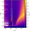 |
Fig. 12 Space-time diagram of the plasma β-parameter for the fiducial model. The red line outlines the regions with β < 6.0. The white line shows the extent of the dead zone defined by Eq. (40). The blue line outlines the outer edge of the disk defined by Σg = 1.0 g cm−2. |
7 Conclusions
We studied numerically the formation and long-term (~ 1.0 Myr) evolution of protoplanetary disks starting from the gravitational collapse of prestellar cores with a special emphasis on the development of MRI-triggered accretion bursts in the innermost disk regions. We employed magnetohydrodynamical simulations in the thin-disk limit adopting the ideal MHD approximation. The numerical model also features the co-evolution of gas and dust including dust backreaction on gas and dust growth.
To simulate the MRI-triggered bursts, we employed the adaptive α-parameter method of Bae et al. (2014), upgraded to take the dependence of the MRI bursts on the magnetic field strength and ionization fraction explicitly into account. In this method, the turbulent α-parameter is a weighted average between αd z = 10−5, corresponding to the MRI-dead disk regions, and αMRI = 10−2–10−1, typical for the fully MRI-active disks. Disk self-gravity was explicitly taken into account via the solution of the Poisson integral. Four models with different masses of prestellar cloud cores ( ) and mass-to-magnetic flux ratios λ were considered. Our main results can be summarized as follows:
A dead zone in the inner disk region forms soon after disk formation, which is characterized by a low ionization fraction (x≲10−13) and temperature on the order of several hundred Kelvin. The outer boundary of the dead zone extends from a few to several tens of astronomical units, depending on
 and λ. The inner boundary coincides with the inner edge of the disk (imposed by the inner numerical boundary at 0.52 au). The dead zone features diffuse gas and sharp dust rings, the latter forming thanks to radial drift of dust toward the local pressure maxima, an effect also predicted in previous studies of dead zones in protoplanetary disks (e.g., Dzyurkevich et al. 2014; Vorobyov et al. 2018; Kadam et al. 2019). In the rest of the disk, however, the dust-to-gas mass ratio drops lower than the initial 1:100 value.
Gradual warming of the dead zone (due to residual viscosity and compressional heating, see Bae et al. 2014) leads to the thermal ionization of alkaline metals and a sharp increase in the ionization fraction. An accretion burst ensues as the inner several astronomical units of the disk become MRI-active and the turbulent viscosity sharply increases. The accretion rate onto the star rises to 5 × 10⁻⁵–
 yr−1 and the accretion luminosity exceeds
  . The burst is characterized by a sharp rise, a plateau with short-term variability, and a fast decline as the inner disk becomes depleted of matter. The concentration of dust in the dead zone assists the warming of the dead zone and the burst triggering by means of the increased optical depth.
The burst occurrence frequency depends on the disk evolutionary stage. Initially, the bursts are difficult to resolve because the innermost disk regions switch frequently from the MRI-dead to the MRI-active state and back. In this very early stage characterized by strong disk mass-loading from the envelope, the accretion is highly variable on 1–2 orders of magnitude. This stage is also deeply embedded and therefore may be difficult to probe observationally. In the subsequent evolution, when the mass infall rate onto the disk begins to decline, individual accretion bursts begin to occur and their frequency declines with time. The dependence of the burst frequency on the evolutionary epoch is likely caused by the disk transition from a highly gravitationally unstable state (in which both gravitational and viscous torques provide fast recharge times for the bursts) to a gravitationally stable state, in which mass is inward-transported only by viscous torques, taking longer recharging times (see also Zhu et al. (2009a).
The burst phenomenon depends on the initial prestellar core mass. It is strongest in more massive cores and virtually diminishes for core masses below
 or the final stellar mass below
  . Objects with these core masses form disks of such a low mass and temperature that the thermal ionization of alkaline metals can hardly be achieved, at least in the considered disk regions beyond 0.5 au.
The burst phenomenon was confirmed to occur for a wide range of the mass-to-flux ratios λ = 2–10. The burst occurrence frequency is weakly affected by the variations of λ in the considered limits.
The MRI-triggered bursts and dust rings in the inner disk regions are intrinsically linked with each other in our model. Both phenomena are a manifestation of the dead zone that forms in the innermost disk regions. However, we should warn against over-interpreting this causal link. Accretion bursts in general and dust rings can be caused by phenomena other than the dead zone. For instance, accretion bursts can be triggered by in-falling gaseous clumps in gravitationally unstable disks (Vorobyov & Basu 2005a, 2015), planet-disk interaction (Lodato & Clarke 2004; Nayakshin & Lodato 2012), or external perturbations (Bonnell & Bastien 1992; Pfalzner et al. 2008; Forgan & Rice 2010). Dust rings can be created, in particular, by planets (Rice et al. 2006; Dong et al. 2015) and snow lines (Zhang et al. 2015). Further studies of the MRI-triggered burst phenomenon are needed to better understand the possible interplay between the dead zone, bursts, and dust rings in protoplanetary disks.
Our model includes many physical effects with different levels of approximations, which may affect our conclusions. The neglect of nonideal MHD effects can influence the distribution of magnetic fields in the disk. More accurate dust opacities that take the dust growth into account are needed to better describe the thermal balance in the disk. The ionization fraction calculations can be improved by including compact chemical reaction networks (see, e.g., Dapp et al. 2012) and thermal sublimation of dust grains. Finally, the dust evolution model would benefit from extension to a full multi-bin version and inclusion of dust ice coating into the calculations of dust fragmentation velocity would allow a more accurate calculation of the maximum size of dust grains (Molyarova et al. 2020).
Acknowledgements
We thank the anonymous referee for useful comments that helped to improve the manuscript. This paper is supported by the Austrian Science Fund (FWF) under research grant I2549-N27 and Swiss National Science Foundation (SNSF) (project number 200021L_163172). The work of Sergey Khaibrakhmanov in Sects. 2.3 and 2.4 is supported by the Large Scientific Project of the Russian Ministry of Science and Higher Education “Theoretical and experimental studies of the formation and evolution of extrasolar planetary systems and characteristics of exoplanets” (project No. 075-15-2020-780, contract 780-10). SB was supported by a Discovery Grant from the Natural Sciences and Engineering Research Council (NSERC) of Canada. The simulations were performed on the Vienna Scientific Cluster (VSC-3 and VSC-4) and on the Shared Hierarchical Academic Research Computing Network (SHARCNET).
References
- Armitage, P. J. 2015, ArXiv e-prints [arXiv:1509.06382] [Google Scholar]
- Armitage, P. 2016, ApJ, 833, 15 [NASA ADS] [CrossRef] [Google Scholar]
- Armitage, P. J., Livio, M., & Pringle, J. E. 2001, MNRAS, 324, 705 [NASA ADS] [CrossRef] [Google Scholar]
- Audard, M., Ábrahám, P., Dunham, M. M., et al. 2014, in Protostars and Planets VI, eds. H. Beuther, R. S. Klessen, C. P. Dullemond, & T. Henning (Tucson, AZ: Univ. Arizona Press), 387 [Google Scholar]
- Bae, J., Hartmann, L., Zhu, Z., & Nelson, R. P. 2014, ApJ, 795, 61 [NASA ADS] [CrossRef] [Google Scholar]
- Bai, X.-N. 2016, ApJ, 821, 80 [Google Scholar]
- Balbus, S. A., & Terquem, C. 2001, ApJ, 552, 237 [NASA ADS] [CrossRef] [Google Scholar]
- Basu, S. 1997, ApJ, 485, 240 [CrossRef] [Google Scholar]
- Bell, K. R., & Lin, D. N. C. 1994, ApJ, 427, 987 [NASA ADS] [CrossRef] [Google Scholar]
- Binney, J., & Tremaine, S. 1987, Galactic Dynamics (Princeton: Princeton University Press) [Google Scholar]
- Birnstiel, T., Klahr, H., & Ercolano, B., 2012, A&A, 539, A148 [NASA ADS] [CrossRef] [EDP Sciences] [Google Scholar]
- Bonnell, I., & Bastien, P. 1992, ApJ, 401, L31 [Google Scholar]
- Booth, R. A., & Clarke, C. J. 2016, MNRAS, 458, 2676 [NASA ADS] [CrossRef] [Google Scholar]
- Caratti o Garatti A., Stecklum, B., Garcia Lopez, R., et al. 2016, Nature Phys., 13, 276 [Google Scholar]
- Cieza, L. A., Casassus, S., Tobin, J., et al. 2016, Nature, 535, 258 [NASA ADS] [CrossRef] [Google Scholar]
- Colella, P., & Woodward, P. R. 1984, J. Comput. Phys., 54, 174 [NASA ADS] [CrossRef] [MathSciNet] [Google Scholar]
- Contreras Peña, C., Lucas, P. W., Minniti, D., et al. 2017, MNRAS, 465, 3011 [NASA ADS] [CrossRef] [Google Scholar]
- Contreras Peña, C., Naylor, T., & Morrell, S. 2019, MNRAS, 486, 4590 [CrossRef] [Google Scholar]
- D’Angelo, C. R., & Spruit, H. C. 2012, MNRAS, 420, 416 [NASA ADS] [CrossRef] [Google Scholar]
- Dapp, W. B., Basu, S., & Kunz, M. W. 2012, A&A, 541, A35 [NASA ADS] [CrossRef] [EDP Sciences] [Google Scholar]
- Dong, R., Zhu, Z., & Whitney, B. 2015, ApJ, 809, 93 [NASA ADS] [CrossRef] [Google Scholar]
- Dong, R., Vorobyov, E., Pavlyuchenkov, Y., Chiang, E., & Liu, H. B. 2016, ApJ, 823, 141 [NASA ADS] [CrossRef] [Google Scholar]
- Drażkowska, J., Li, S., Birnstiel, T., Stammler, S. M., & Li, H. 2019, ApJ, 885, 91 [NASA ADS] [CrossRef] [Google Scholar]
- Dudorov, A. E., 1995, Astron. Rep., 39, 790 [Google Scholar]
- Dudorov, A. E., & Sazonov, Y. V. 1987, Nuch. Inform., 63, 68 [Google Scholar]
- Dudorov, A. E., & Khaibrakhmanov, S. 2014, Ap&SS, 352, 103 [NASA ADS] [CrossRef] [Google Scholar]
- Dzyurkevich, N., Flock, M., Turner, N. J., Klahr, H., & Henning, Th. 2010, A&A, 515, A70 [NASA ADS] [CrossRef] [EDP Sciences] [Google Scholar]
- Elbakyan, V. G., Vorobyov, E. I., Rab, C., Meyer, D. M.-A., Güdel, M., et al. 2019, MNRAS, 484, 146 [NASA ADS] [CrossRef] [Google Scholar]
- Fischer, W. J., Safron, S., & Megeath, S. Th. 2019, ApJ, 872, 183 [CrossRef] [Google Scholar]
- Forgan, D., & Rice, K. 2010, MNRAS 402, 1349 [NASA ADS] [CrossRef] [Google Scholar]
- Gammie, C. 1996, ApJ, 457, 355 [NASA ADS] [CrossRef] [Google Scholar]
- Güdel, M., Eibensteiner, C., Dionatos, O., et al. 2019, A&A, 631, A8 [CrossRef] [EDP Sciences] [Google Scholar]
- Hawley, J. F., Gammie, C. F., & Balbus, S. A. 1995, ApJ, 440, 742 [NASA ADS] [CrossRef] [Google Scholar]
- Hillenbrand, L. A., & Findeisen, K. P. 2015, ApJ, 808, 68 [NASA ADS] [CrossRef] [Google Scholar]
- Hubbard, A. 2016, MNRAS, 465, 1910 [NASA ADS] [CrossRef] [Google Scholar]
- Kadam, K., Vorobyov, E. I., Regály, Z., Kóspál, Á., & Abrahám, P. 2019, ApJ, 882, 96 [NASA ADS] [CrossRef] [Google Scholar]
- Kadam, K., Vorobyov, E. I., Regály, Z., Kóspál, Á., & Abrahám, P. 2020, ApJ, 895, 41 [CrossRef] [Google Scholar]
- Kóspál, Á., Szabó, Zs. M., Ábrahám, P., et al. 2020, ApJ, 889, 148 [CrossRef] [Google Scholar]
- Kratter, K., & Lodato, G. 2016, ARA&A, 54, 271 [NASA ADS] [CrossRef] [Google Scholar]
- Kuffmeier, M., Frimann, S., Jensen, S. S., & Haugbølle, T. 2018, MNRAS, 475, 2642 [NASA ADS] [CrossRef] [Google Scholar]
- Kunz, M. W., & Balbus, S. A. 2004, MNRAS, 348, 355 [NASA ADS] [CrossRef] [Google Scholar]
- Lee, J.-E., Lee, S., Baek, G., et al. 2019, Nat. Astron., 3, 314 [NASA ADS] [CrossRef] [Google Scholar]
- Lodato, G., & Clarke, C. J. 2004, MNRAS, 353, 841 [NASA ADS] [CrossRef] [Google Scholar]
- Machida, M. N., Inutsuka, S., & Matsumoto, T. 2011a, ApJ, 724, 1006 [Google Scholar]
- Machida, M. N., Inutsuka, S., & Matsumoto, T. 2011b, ApJ, 729, 42 [NASA ADS] [CrossRef] [Google Scholar]
- Martin, R. G., Lubow, S. H., Livio, Mario, & Pringle, J. E. 2012a, MNRAS 420, 3139 [NASA ADS] [CrossRef] [Google Scholar]
- Martin, R. G., Lubow, S. H., Livio, M., & Pringle, J. E. 2012b, MNRAS, 423, 2718 [NASA ADS] [CrossRef] [Google Scholar]
- Masset, F. 2000, A&ASS, 141, 165 [NASA ADS] [CrossRef] [EDP Sciences] [Google Scholar]
- Meyer, D. M.-A., Vorobyov, E. I., Kuiper, R., Kley, W., 2017, MNRAS, 464, L90 [NASA ADS] [CrossRef] [Google Scholar]
- Molyarova, T., Vorobyov, E. I., Akimkin, V., Skliarevskii, A., Wiebe, D., & Guedel, M. 2020, ApJ, submitted [Google Scholar]
- Nakano, T. 1984, Fundam. Cosmic Phys. 9, 139 [Google Scholar]
- Nayakshin, S.,& Lodato, G. 2012, MNRAS, 426, 70 [NASA ADS] [CrossRef] [Google Scholar]
- Pfalzner, S., Tackenberg, J., & Steinhausen, M. 2008, A&A, 487, L45 [NASA ADS] [CrossRef] [EDP Sciences] [Google Scholar]
- Riaz, R., Vanaverbeke, S., & Schleicher, D. R. G., 2018, A&A, 614, A53 [CrossRef] [EDP Sciences] [Google Scholar]
- Rice, W. K. M., Lodato, G., Pringle, J. E., Armitage, P. J., & Bonnell, I. A. 2004, MNRAS, 355, 543 [NASA ADS] [CrossRef] [Google Scholar]
- Rice, W. K. M., Armitage, P. J., Wood, K., & Lodato, G. 2006, MNRAS, 373, 1619 [Google Scholar]
- Richtmyer, R. D., & Morton, K. W. 1967. Difference Methods for Initial-value Problems (New York: Interscience) [Google Scholar]
- Sano, T., Miyama, S. M., Umebayashi, T., & Nakano, T. 2000, ApJ, 543, 486 [NASA ADS] [CrossRef] [Google Scholar]
- Scholz, A., Froebrich, D., & Wood, K. 2013, MNRAS, 430, 2910 [NASA ADS] [CrossRef] [Google Scholar]
- Semenov, D., Henning, T., Helling, C., Ilgner, M., & Sedlmayr, E. 2003, A&A, 410, 611 [NASA ADS] [CrossRef] [EDP Sciences] [Google Scholar]
- Shakura, N. I., & Sunyaev, R. A. 1973, A&A, 24, 337 [NASA ADS] [Google Scholar]
- Spitzer, L. 1978 Physical Processes in the Interstellar Medium (New York: Wiley) [Google Scholar]
- Stepinski, T. F., & Valageas, P. 1997, A&A, 319, 1007 [NASA ADS] [Google Scholar]
- Stone, J. M., & Norman, M. L. 1992, ApJSS, 80, 753 [NASA ADS] [CrossRef] [Google Scholar]
- Stone, J. M., & Norman, M. L. 1992, ApJSS, 80, 791 [NASA ADS] [CrossRef] [Google Scholar]
- Stoyanovskaya, O. P., Vorobyov, E. I., & Snytnikov, V. N., 2018, Astron. Rep., 62, 455 [NASA ADS] [CrossRef] [Google Scholar]
- Stoyanovskaya, O. P., Okladnikov, F. A., Vorobyov, E. I., Pavlyuchenkov, Ya. N., & Akimkin, V. V. 2020, Astron. Rep., 64, 107 [CrossRef] [Google Scholar]
- Suzuki, T. K., Ogihara, M., Morbidelli, A., Crida, A., & Guillot, T. 2016, A&A, 596, A74 [NASA ADS] [CrossRef] [EDP Sciences] [Google Scholar]
- Taquet, V., Wirström, E. S., & Charnley, S. B. 2016, ApJ, 821, 46 [NASA ADS] [CrossRef] [Google Scholar]
- Umebayashi, T., & Nakano, T. 2009, ApJ, 690, 69 [NASA ADS] [CrossRef] [Google Scholar]
- Vorobyov, E. I., & Basu, S. 2005a, ApJ, 633, L137 [NASA ADS] [CrossRef] [Google Scholar]
- Vorobyov, E. I., & Basu, S. 2005b, MNRAS, 360, 675 [NASA ADS] [CrossRef] [Google Scholar]
- Vorobyov, E. I., & Basu, S. 2009, MNRAS, 393, 822 [NASA ADS] [CrossRef] [Google Scholar]
- Vorobyov, E. I., & Basu, S. 2010, ApJ, 719, 1896 [NASA ADS] [CrossRef] [Google Scholar]
- Vorobyov, E. I., & Basu, S. 2015, ApJ, 805, 115 [NASA ADS] [CrossRef] [Google Scholar]
- Vorobyov, E. I., Akimkin, A., Stoyanovskaya, O. P., Pavlyuchenkov, Ya., & Liu, H. B. 2018, A&A, 614, A98 [NASA ADS] [CrossRef] [EDP Sciences] [Google Scholar]
- Vorobyov, E. I., Skliarevskii, A. M., Elbakyan, V. G., Pavlyuchenkov, Ya., Akimkin, V., & Guedel, M. 2019, A&A, 627, A154 [NASA ADS] [CrossRef] [EDP Sciences] [Google Scholar]
- Wiebe, D. S., Molyarova, T. S., Akimkin, V. V., Vorobyov, E. I., & Semenov, D. A. 2019, MNRAS, 485, 1843 [CrossRef] [Google Scholar]
- Yang, C.-C., Mac Low, M.-M., & Johansen, A. 2018, ApJ, 868, 27 [NASA ADS] [CrossRef] [Google Scholar]
- Yorke, H. W., & Bodenheimer, P., 2008, ASP Conf. Ser., 387, 189 [Google Scholar]
- Zhang, K., Blake, G. A., & Bergin, E. A. 2015, ApJ, 806, L7 [NASA ADS] [CrossRef] [Google Scholar]
- Zhu, Z., Hartmann, L., & Gammie, C. 2009a, ApJ, 694, 1045 [NASA ADS] [CrossRef] [Google Scholar]
- Zhu, Z., Hartmann, L., Gammie, C., & McKinney, J. C. 2009b, ApJ, 701, 620 [NASA ADS] [CrossRef] [Google Scholar]
- Zhu, Z., Jiang, Y.-F., & Stone, J. M. 2020, MNRAS, 495, 3494 [CrossRef] [Google Scholar]
The cooling and heating rates in Dong et al. (2016) are written for one side of the disk and need to be multiplied by a factor of 2.
When deriving Eq. (46) we assumed that  . In massive disks with
  a more accurate but complex expression should be used (see Eq. (11) in Kratter & Lodato 2016).
All Tables
All Figures
|
Fig. 1 Azimuthally averaged radial profiles of the gas surface density (panel a), temperature (panel b), gas radial (panel c) and azimuthal velocities (panel d) at different evolution times after the onset of the simulation (1: 0 kyr, 2: 54.9 kyr, 3: 55.1 kyr, 4: 56.0 kyr, 5: 56.2 kyr, 6: 156.2 kyr). The black dashed lines with labels show typical slopes. |
| In the text | |
|
Fig. 2 Two-dimensional distribution of the gas surface density in inner 600 × 600 au2 box at time instances 0.049, 0.099, 0.149, 0.199, 0.349, 0.549 Myr after disk formation. White contours mark the disk loci with Σ = 1 g cm−2. The time is counted from the disk formation instance (t = 0.056 Myr). |
| In the text | |
|
Fig. 3 Two-dimensional distribution of the grown dust surface density in the inner 6 × 60 au2 box at time instances 0.049, 0.099, 0.149, 0.199, 0.349, 0.549 Myr after disk formation. The time is counted from the disk formation instance. |
| In the text | |
|
Fig. 4 Azimuthally averaged dust characteristics at t = 0.199 Myr (left column) and t = 0.549 Myr (right column) from the instance of disk formation. Top row: presents the surface densities of small and grown dust and also the vertically integrated gas pressure. Bottom row: shows the dust radius, Stokes number, and total dust-to-gas ratio. |
| In the text | |
|
Fig. 5 Space-time diagrams of the azimuthally averaged radial profiles for the gas and grown dust surface densities (left and right panels, respectively). The white contour line indicates the disk loci with Σg = 1.0 g cm−2. |
| In the text | |
|
Fig. 6 Space-time diagrams of the azimuthally averaged radial profiles of temperature and
|
| In the text | |
|
Fig. 7 Top left (a): the accretion rate onto the star versus time starting from disk formation. Bottom left (b): similar to the top-left panel, but for a time interval t = [0.149, 0.150] Myr. Orange rectangles mark the burst analyzed in Fig. 8. Right (c): space–time diagram of the azimuthally averaged ionization fraction. The white contour line delineates the dead zone boundary. The time is counted from the instance of disk formation. |
| In the text | |
|
Fig. 8 Upper panel: accretion rate onto the star versus time in the time interval t = [0.149, 0.150] Myr after the disk formation. Lower rows of panels: two-dimensional distributions of the ionization fraction (first row), turbulent parameter α (second row), and gas temperature (third row) in the region r ≤ 30 au at time instants t = 0.1491, 0.1493 and 0.1497 Myr marked with blue rounds with labels “A”, “B” and “C” in the upper panel, respectively. The white contour delineates the boundary of the dead zone. |
| In the text | |
|
Fig. 9 Time evolution of several disk and burst characteristics at the sink–disk interface as the burst develops and decays. Shown are the mass accretion rate (top-left), total luminosity (top-right), midplane temperature (middle-left), gas and grown dust surface densities (middle-right), α-value (bottom-left), and ionization fraction (bottom-right). |
| In the text | |
|
Fig. 10 Protostellar accretion rates (black lines) and envelope infall rates (red lines) as a function of time in models with various initial pre-stellar come masses and mass-to-flux ratios: model 1 –
|
| In the text | |
|
Fig. 11 Space-time diagrams showing the ionization fraction in model 2L (left) and model 3 (right). The white contour lines delineate the position of the dead zone. |
| In the text | |
|
Fig. 12 Space-time diagram of the plasma β-parameter for the fiducial model. The red line outlines the regions with β < 6.0. The white line shows the extent of the dead zone defined by Eq. (40). The blue line outlines the outer edge of the disk defined by Σg = 1.0 g cm−2. |
| In the text | |
Current usage metrics show cumulative count of Article Views (full-text article views including HTML views, PDF and ePub downloads, according to the available data) and Abstracts Views on Vision4Press platform.
Data correspond to usage on the plateform after 2015. The current usage metrics is available 48-96 hours after online publication and is updated daily on week days.
Initial download of the metrics may take a while.