| Issue |
A&A
Volume 644, December 2020
|
|
|---|---|---|
| Article Number | A32 | |
| Number of page(s) | 13 | |
| Section | Cosmology (including clusters of galaxies) | |
| DOI | https://doi.org/10.1051/0004-6361/202038508 | |
| Published online | 26 November 2020 | |
A novel CMB polarization likelihood package for large angular scales built from combined WMAP and Planck LFI legacy maps
1
Dipartimento di Fisica e Scienze della Terra, Università degli Studi di Ferrara, Via Giuseppe Saragat 1, 44122 Ferrara, Italy
e-mail: This email address is being protected from spambots. You need JavaScript enabled to view it.
, This email address is being protected from spambots. You need JavaScript enabled to view it.
2
Istituto Nazionale di Fisica Nucleare (INFN), Sezione di Ferrara, Via Giuseppe Saragat 1, 44122 Ferrara, Italy
3
Dipartimento di Fisica, Università di Roma Tor Vergata, Via della Ricerca Scientifica 1, 00133 Roma, Italy
4
Istituto Nazionale di Fisica Nucleare (INFN), Sezione di Roma 2, Via della Ricerca Scientifica 1, 00133 Roma, Italy
5
Dipartimento di Fisica, Università degli Studi di Milano, Via Celoria 16, 20133 Milano, Italy
6
INAF – OAS Bologna, Istituto Nazionale di Astrofisica – Osservatorio di Astrofisica e Scienza dello Spazio di Bologna, Via Gobetti 101, 40129 Bologna, Italy
7
Istituto Nazionale di Fisica Nucleare (INFN), Sezione di Bologna, viale Berti Pichat 6/2, 40127 Bologna, Italy
8
Space Science Data Center – Agenzia Spaziale Italiana, Via del Politecnico snc, 00133 Roma, Italy
Received:
27
May
2020
Accepted:
29
July
2020
Abstract
We present a cosmic microwave background (CMB) large-scale polarization dataset obtained by combining Wilkinson Microwave Anisotropy Probe (WMAP) in the K, Q, and V bands with the Planck 70 GHz maps. We employed the legacy frequency maps released by the WMAP and Planck collaborations and performed our own Galactic foreground mitigation technique, relying on Planck 353 GHz for polarized dust and on Planck 30 GHz and WMAP K for polarized synchrotron. We derived a single, optimally noise-weighted, low residual foreground map and the accompanying noise covariance matrix. These are shown through χ2 analysis to be robust over an ample collection of Galactic masks. We used this dataset, along with the Planck legacy Commander temperature solution, to build a pixel-based low-resolution CMB likelihood package, whose robustness we tested extensively with the aid of simulations, finding an excellent level of consistency. Using this likelihood package alone, we are able to constrain the optical depth to reionization, τ = 0.069−0.012+0.011 at 68% confidence level, on 54% of the sky. Adding the Planck high-ℓ temperature and polarization legacy likelihood, the Planck lensing likelihood, and BAO observations, we find τ = 0.0714−0.0096+0.0087 in a full ΛCDM exploration. The latter bounds are slightly less constraining than those obtained by employing the Planck High Frequency Instrument’s (HFI) CMB data for large-angle polarization, which only include EE correlations. Our bounds are based on a largely independent dataset that includes TE correlations. They are generally compatible with Planck HFI, but lean towards slightly higher values for τ. We have made the low-resolution Planck and WMAP joint dataset publicly available, along with the accompanying likelihood code.
Key words: cosmological parameters / dark ages / reionization, first stars
© ESO 2020
1. Introduction
Measuring the cosmic microwave background (CMB) polarization at large angular scales is crucial for constraining the reionization peak and, in particular, for the determination of the Thomson scattering optical depth to reionization, τ, which is currently the less constrained of the ΛCDM parameters. The optical depth, τ, is connected to the integrated amount of free electrons along the line of sight and provides information on how and when the first stars and galaxies formed.
Remarkable advancements have been made in this field over the last 15 years. The Wilkinson Microwave Anisotropy Probe (WMAP) (Hinshaw et al. 2013) and Planck (Planck Collaboration VI 2020) collaborations have continuously improved the quality of large-scale polarization measurements, which are known to be notoriously extremely tough to clean from contaminations coming from the foreground and instrumental systematic effects. The most constraining dataset currently available is provided by the Planck collaboration (Planck Collaboration I 2020), which uses the High Frequency Instrument (HFI) measurements at 100 and 143 GHz. Such results for the Legacy Planck release are presented in Planck Collaboration III (2020) and Planck Collaboration V (2020), while an improved post-Planck analysis is presented in Delouis et al. (2019) and in Pagano et al. (2020).
These HFI-based measurements are all specifically designed to determine the reionization optical depth and, thus, they are mainly dedicated to the characterization of the E-modes power spectrum. This approach, which is consistent with the corresponding likelihood codes delivered, is mainly driven by the difficulty of building reliable noise covariance matrices and by the relatively high level of residual systematic effects related to dipole and foreground temperature-to-polarization leakage. Such likelihoods, despite being the most sensitive to date, do not include the TE spectrum Planck Collaboration V (2020). Furthermore, they cannot be adapted to handle non-rotationally invariant cosmologies in a straightforward way and they might need tuned-up simulations for exotic models (see Planck Collaboration V 2020, Sect. 2.2.6).
For the Legacy data release, together with the HFI-based likelihood, the Planck collaboration has also delivered a map-based likelihood employing observations of the Low Frequency Instrument (LFI) in the 70 GHz channel. The sensitivity to the reionization optical depth of the LFI-based likelihood is inferior by more than a factor of two with respect to the HFI-based likelihood.
The possibility of combining the WMAP and Planck observations to build a “joint” dataset that is more constraining was first explored by some of our team in Lattanzi et al. (2017), using the data available at the time. To date, however, a combined dataset using the WMAP and Planck legacy observations of the large-scale polarization is not publicly available. Aiming to fill this gap, here we present a combined real-space polarization dataset which jointly considers the Planck 70 GHz channel and the WMAP Ka, Q, and V bands. Because of the aforementioned difficulty in dealing with residual systematic effects in the pixel space (Planck Collaboration V 2020), we do not consider the HFI CMB channels, such as 100 and 143 GHz.
An important aspect of our work is that we perform an independent analysis pipeline starting from the raw maps, as delivered by the two collaborations. From there, we build polarization masks, perform foreground cleaning through a template fitting and, finally, combine the four maps in the pixel domain through inverse noise weighting. The resulting dataset, despite still having an overall higher noise than the HFI-based one, allows for an independent estimation of the reionization optical depth. Moreover, being a real-space dataset, it is suitable for a number of studies that are not accessible for a spectrum-based likelihood (see, e.g., Planck Collaboration XXIII 2014; Planck Collaboration XVI 2016) and it is capable of exploring non-rotationally invariant cosmologies. For an exhaustive review of likelihood methods, see Gerbino et al. (2020).
The paper is organized as follows. We start by describing the input datasets in Sect. 2. In Sect. 3, we present the new set of masks produced for the Planck and WMAP data. In Sect. 4, we introduce the main algorithms used in the paper, including a detailed discussion of the role of the regularization noise used in the analysis. In Sect. 5, we present the results of the component separation process. In Sects. 6 and 7, we show the angular power spectra and study the stability of the τ estimates in different masks, in addition to performing a Monte Carlo validation. We present our constraints on the reionization optical depth, τ, in Sect. 8 and we draw our conclusions in Sect. 9.
2. Datasets
In this section, we describe the large-scale WMAP and Planck polarization maps that were used to build the combined dataset. As already mentioned, as CMB channels, we considered the 70 GHz channel from Planck LFI (Planck Collaboration II 2020) and the Ka, Q, and V bands from WMAP (Bennett et al. 2013). In the case of LFI 70 GHz, we used the full mission map after removing the bandpass and gain-mismatch-leakage correction maps. These maps, described in Planck Collaboration II (2020), are part of the Planck 2018 legacy data release, and are publicly available through the Planck Legacy Archive1. For WMAP, we use the raw nine-year frequency maps, available on the Lambda archive2. In principle, we could have also considered the 44 GHz channel from Planck LFI and the W-band from WMAP as CMB channels. However, we found that both these channels show excess power, likely to be spurious in origin, after implementing the foreground cleaning procedure described in Sect. 4. For this reason, we decided not to include the 44 GHz and W-band channels in our analysis. We note that the Planck and WMAP collaborations made the same choice on similar grounds (Planck Collaboration V 2020; Page et al. 2007).
We employed the K-band from WMAP, LFI 30 GHz, and HFI 353 GHz maps from Planck as tracers of Galactic foreground emission. These are used both to generate masks excluding regions dominated by Galactic emissions, and to mitigate the astrophysical foreground contamination in the remaining parts of the sky, as explained in detail in Sects. 3 and 4. At 30 GHz, we used the full-mission, bandpass leakage-corrected map. For the 353 GHz channel, we selected a map built only from data provided by polarization-sensitive bolometers (PSB; Planck Collaboration III 2020), as done in the low-ℓ analysis presented in Planck Collaboration V (2020). The WMAP K band and Planck 30 GHz are used as a polarized synchrotron tracer, respectively, for the WMAP and Planck CMB channels. This follows the prescription of Lattanzi et al. (2017) and Weiland et al. (2018). The Planck 353 GHz is used as polarized thermal dust tracer for both WMAP and Planck.
Since we are mainly focused on the large angular scales, it appears convenient to work with low-resolution datasets. Thus, all the maps of the Stokes parameters, m = [Q, U], describing the measured linear polarization, were downgraded to a HEALPix resolution of Nside = 16 (Górski et al. 2005), which corresponds to a pixel size of ∼3.7 degrees. A smoothing kernel was applied to the high-resolution maps prior to the downgrading, which is meant to avoid aliasing into the large angular scales of the high-frequency power present in the maps. The smoothing was performed in harmonic space, using a cosine window function (Benabed et al. 2009; Planck Collaboration V 2020). This guarantees that the signal is left unaltered on the scales of interest, that is, up to multipoles of ℓ = Nside = 16, while it is smoothly set to zero on smaller scales, ℓ > 3 × Nside = 48.
The instrumental noise properties of each low-resolution map are described by an associated pixel-pixel noise covariance matrix (NCVM). For the LFI channels, the covariance matrices are presented in Planck Collaboration II (2020). The 70 GHz covariance matrix has been rescaled in harmonic space in order to match the noise level of the half-difference of half-ring maps, following the procedure described in Planck Collaboration V (2020). For the HFI 353 GHz NCVM, we use a downgraded version of the map-making covariance matrix, which is instead generated at the native high-resolution of Nside = 2048. This NCVM only accounts for Q and U correlations within the same pixel, while correlations between different pixels are ignored. Finally, for WMAP we build the NCVMs starting from the polarization pixel-pixel inverse covariance matrices at Nside = 16 (Res 4) delivered by the WMAP team and described in Page et al. (2007), Bennett et al. (2013). The cosine window function apodization is performed in harmonic space on the eigenvectors of these low resolution matrices. It is worth noting that although exchanging the order of the smoothing and downgrading operations is clearly not an option at the map level, due to the possible presence of sub-pixel structure, it can still be acceptable for the NCVMs.
Since all the (Q,U) NCVMs were convolved with a smoothing function, we added to them a white noise covariance matrix, with σ2 = (20 nK)2, in order to guarantee that they are numerically well-conditioned, as in Planck Collaboration V (2020). For consistency, noise with the same statistical properties has to be added to the corresponding maps. However, instead of adding a single noise realization to each smoothed data map, as in Planck Collaboration V (2020), we followed a different procedure, which is described in Sect. 4. This ensures that our results are not biased by a particular realization of the regularization noise.
Concerning the temperature (T) map, we always employ the Planck 2018 Commander solution (Planck Collaboration IV 2020) outside its confidence mask, which leaves 86% of the sky available. This map was filtered with a Gaussian beam of FWHM 440 arcmin and downgraded to Nside = 16. Since it is reasonable to assume that the temperature noise at large angular scales is negligible, we only need to include the regularization noise. Thus, we modeled the temperature NCVM as a white noise covariance matrix with σ2 = (2 μK)2, as in Planck Collaboration V (2020). We consistently handle such regularization noise following the same procedure adopted for polarization. Finally, when building the NCVM of the full TQU maps, we neglect the correlation between temperature and polarization and set the corresponding off-diagonal blocks in the covariance matrix to zero (Planck Collaboration XI 2016).
3. Polarization masks
In order to efficiently perform the foreground cleaning and the cosmological parameter estimation, we must remove the pixels of the data map that are most affected by foreground contamination from the analysis. With regard to temperature, we always use the Commander 2018 confidence mask (Planck Collaboration V 2020) provided by the Planck collaboration. In this section, we describe how the polarization masks are produced.
In polarization, we built two different sets of masks for WMAP and LFI. For LFI 70 GHz, we used the 30 and the 353 GHz maps as, respectively, synchrotron (s) and dust (d) tracers, analagously to what is done in Planck Collaboration V (2020). We first applied a Gaussian smoothing with a full width half maximum (FWHM) of 7.5° to these input maps, taken at their native resolution of Nside = 1024 (30 GHz) and Nside = 2048 (353 GHz). Then we built maps of the polarization amplitude  and
and  , where the scaling coefficients are set to α = 0.063 and β = 0.0077, as estimated in Planck Collaboration XI (2016). These two maps were subsequently downgraded to the HEALPix resolution Nside = 16. From these maps, two separate sets of masks for synchrotron and dust emission were built as follows. We excluded pixels where the relevant polarization intensity, Ps or Pd, is greater than a given threshold. This threshold is expressed in terms of excess intensity with respect to the corresponding mean value, ⟨Ps⟩ or ⟨Pd⟩, over the whole sky. Any pair of synchrotron and dust masks can then be combined to yield a single foreground mask. Varying the threshold, we were able to build foreground masks keeping a chosen fraction of the sky. We chose to build, for LFI 70 GHz, nine different masks with equally spaced sky fractions fsky = 30%, 35%, …, 65%, 70%. We did not consider larger sky fractions because, as we show in Sect. 5, we find an indication of excess residual power in the LFI maps after foreground removal for masks with fsky > 60%. A subset of the LFI masks is shown in Fig. 1.
 |
Fig. 1. Subset of the masks used in the analysis of the LFI 70 GHz data. Values of the available sky fraction fsky in each mask are 30%, 40%, 50%, and 60%. |
Foreground scalings coefficients from WMAP K-band (α) and Planck 353 GHz (β) to the indicated WMAP channels.
A corresponding set of masks for WMAP channels is built through a similar procedure. Here, we use the WMAP K-band as a tracer for synchrotron emission and Planck 353 GHz for dust. These are rescaled using the coefficients in Lattanzi et al. (2017); for completeness, these values are also reported in Table 1 here. In this case, when the mask structure at intermediate and high latitudes is dominated by the synchrotron emission (i.e., by the K-band). Thus we decided to adopt the same mask for the three WMAP bands. This leads to a single set of ten masks, with a sky fraction ranging from 30% to 75% in steps of 5%. A subset of the masks is shown in Fig. 2.
 |
Fig. 2. Subset of the masks used in the analysis of the WMAP data. Values of the available sky fraction fsky in each mask are 30%, 40%, 50%, and 60%. |
Finally, with the aim of building a WMAP-Planck LFI combined dataset, we also produced another set of masks to be used in the analysis of the joint dataset. These were built by combining pairs of WMAP and LFI masks, taking the pixels that are left available in at least one of the two masks. In other words, if we think of a mask as the set of all pixels that can be used in the analysis, the “joint” masks are the union (in the set-theory meaning of the word) of the individual WMAP and LFI masks. For this reason, the sky fraction of each combined mask is always equal or larger than the sky fractions of the individual masks it is built from. For example, the union of the WMAP and Planck LFI 30% masks has fsky ≃ 35%. We then chose to produce a set of ten masks built as follows. The first seven masks are the union of each pair of WMAP and Planck masks with the same sky fraction fsky = 30%, 35%, …, 55%,60%. The remaining three masks are the union of the LFI 60% mask with the WMAP 65%, 70% and 75% masks. The reason behind this choice is, as mentioned above and discussed in more detail in Sect. 6, that we do not consider the LFI masks with fsky > 60% to be suitable for cosmological analyses. The sky fractions for the set of union masks, together with the individual masks used to produce them, are summarized in Table 2.
Masks used in the analysis of the joint WMAP-Planck dataset.
4. Methods
In this section, we describe the cleaning procedure and the likelihood approximation used in cosmological parameter estimation. We pay particular attention to the impact of regularization noise on both scalings and cosmological parameters estimation and, at the end of the section, we discuss how it can be mitigated.
The cleaning procedure adopted here is based on fitting foreground templates at the map level (see, e.g., Page et al. 2007; Planck Collaboration XI 2016; Planck Collaboration V 2020). Denoting the linear polarization map at a given frequency, ν, with ![Mathematical equation: $ {\mathbf{m}^{P}_\nu} = \left[{\mathbf{Q}}_\nu,\,{\mathbf{U}}_\nu\right] $](/articles/aa/full_html/2020/12/aa38508-20/aa38508-20-eq5.gif) , the corresponding foreground-cleaned map
, the corresponding foreground-cleaned map  is3
is3
 (1)
(1)
where ts (td) and αν (βν) are the tracers and the scaling coefficient for synchrotron (dust) emission, respectively, described in Sect. 2. Thus, if SP and  are, respectively, the signal and noise covariance matrices at frequency, ν, the fitted coefficients in Eq. (1) are estimated by minimization of the quantity:
 (2)
(2)
where  is the covariance matrix,
 (3)
(3)
We note that  is a χ2-distributed quantity when considered as a function of the map but not as a function of the scalings.
Here, Ns and Nd are the polarization parts of the NCVMs for the foregrounds tracers. The signal covariance matrix is built as described in Tegmark & de Oliveira-Costa (2001) and assumes a fiducial power spectrum,  , taken as the Planck legacy best-fit (Planck Collaboration VI 2020). The inversion of
  , needed to compute the χ2 in Eq. (2), requires the addition of some regularization noise. In particular, we follow the approach used in the Planck legacy analysis (Planck Collaboration XI 2016; Planck Collaboration VI 2020) and consider white noise in polarization with rms
  . We thus sum a random white noise realization,
  , with this amplitude to
  and add a diagonal term,
  , to the covariance matrix (3) and then use these regularized objects to build the χ2 in Eq. (2). In the following, we denote the cleaned map with regularization noise added as
  and the associated covariance matrix as
  .
.
Once αν and βν have been estimated through this minimization procedure, we can define the cleaned data vector ![Mathematical equation: $ {{\mathbf{m}}^\mathrm{fc}_\nu}\equiv\left[ {\mathbf{T}},\,{{\bf m}^{P,{\rm fc}}_\nu} \right] $](/articles/aa/full_html/2020/12/aa38508-20/aa38508-20-eq21.gif) , with T being the Commander map described in Sect. 2. We write down its likelihood function (Gerbino et al. 2020),
, with T being the Commander map described in Sect. 2. We write down its likelihood function (Gerbino et al. 2020),  , as
, as
 (4)
(4)
The NCVM  used in the likelihood analysis is built as follows. The TT block is consistent with the Commander map having only white regularization noise with rms
  , while the TQ and TU blocks are vanishing. The polarization part
  of the NCVM is instead given by
 (5)
(5)
where σαν and σβν are the uncertainties in the estimates of foreground scaling coefficients and ts, d(ts, d)⊤ is the outer product of the tracer maps.
The addition of regularization noise has a small, but not completely negligible, impact on the determination of the foreground scaling coefficients, and, consequently, on cosmological parameter estimates. In fact, the extra noise added to the map increases the scatter of point estimates (e.g., the posterior mean) of parameter values around the true value. Moreover, the extra term added to the NCVM increases parameter uncertainties. In what follows, we first assess the magnitude of the former effect at the level of both scaling coefficients and cosmological parameters. We then illustrate how we manage to avoid extracting a particular noise realization, which leads to non-negligible scatter (as compared to the one caused by instrumental noise).
In order to show and quantify the extra scatter in the estimates of α, β and cosmological parameters induced by regolarization noise, we proceed as follows. We draw 1000 white noise realizations, nr, i (i = 1, …, 1000), with an rms of 2 μK in temperature and 20 nK in polarization. We then estimate α and β on the Planck 70 GHz channel, following the procedure illustrated above, using each of the realization just described as the regularization noise map. For the sake of this test, we adopt a mask that retains 50% of the sky. This procedure results in 1000 Monte Carlo estimates, αi and βi. Once the scaling coefficients have been obtained, we further proceed with an estimation of the cosmological parameters (log(1010As))i and τi from the likelihood in Eq. (4). We note that in this last step, we consistently use the same regularization noise used when fitting the scaling coefficients.
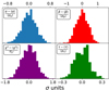 |
Fig. 3. Histograms of the expected scatter in the recovered foreground scalings, in the χ2 of the component separation and in the measured τ due to the regularization noise. For each quantity, we show the distance from the center of the empirical distribution in units of σ. |
Since the CMB signal and the instrumental noise are the same in each map belonging to this ensemble, the scatter in the recovered values of the parameters provides an estimate of the dependence on the regularization noise realization, at the level of both scalings and cosmological parameters. The results of this procedure are shown in Fig. 3, where we show the distribution of the αi’s, βi’s, and τi’s with respect to the mean value, in units of the average uncertainty. We also show the χ2 computed from Eq. (2) in units of  .
.
We then compute their standard deviation, that is,  , where θ = {α ,β ,χ2 ,τ}. For the synchrotron scaling coefficient, α, the scatter induced by the extra noise is, on average, 0.27 times the average parameter uncertainty. In other words, 68% of the αi deviates from ⟨α⟩ by less than 0.27 × ⟨σα⟩. The corresponding value for β is 0.38 times the average parameter uncertainty. The χ2 of the cleaned map is the most affected quantity by the particular realization of regularization noise. In fact, the impact is, at the 1σ level, at most 0.55 times the expected width of a χ2 distribution with Nd.o.f. degrees of freedom. This extra scatter in the scaling estimates induces a smaller, but still non-negligible, effect on the final τ determination. The effect on τ, at one standard deviation of the distribution, equals 11% of its average uncertainty.
Thus, when we add regularization noise, we pay the price of an increased parameter uncertainty, and we might also be prone to unwanted parameter shifts caused by an unlucky choice of the actual noise realisation used. For example, a 3-σ noise realization can easily shift the scalings by ∼1σ and τ by 0.3σ. In fact roughly 1% of the noise realizations in our Monte Carlo resulted in shifts larger than 1 and 0.3σ’s for the scalings and τ, respectively.
A possible way to avoid large parameter shifts is to somehow average over different realizations of the regularization noise. In order to do so, we draw Nit = 1000 white noise realizations nr, i (i = 1, …, 1000) with 20 nK rms. For given values of α and β, these are used to build as many cleaned polarization maps  and the following quantity:
 (6)
(6)
We note that  does not follow a chi-square distribution. It is straightforward to show that its expectation value over the regularization noise is
 (7)
(7)
which is the same as the expectation value of the χ2 built from a single regularized map, χ2 = (mP, fc)⊤C−1mP, fc. Also, this expectation value is different from the value of the χ2 on the regularization noise-free map,
 . The variance associated to
  is:
is:
![Mathematical equation: $$ \begin{aligned} \mathrm{Var} \left[\, \overline{\chi ^2}\,\right]_\mathbf{n _{r}} = \frac{1}{N_{it}}\Bigg \{4 \left(\widetilde{\mathbf{m}}^{P,\mathrm{fc}}\right)^\top {\mathrm{C} }^{-1}{N}^{P}_\mathrm{r} {\mathrm{C} }^{-1}\widetilde{\mathbf{m}}^{P,\mathrm{fc}}+2 \mathrm{Tr} \left[\left( {\mathrm{C} }^{-1}{N}^{P}_\mathrm{r} \right)^2\right]\Bigg \} \end{aligned} $$](/articles/aa/full_html/2020/12/aa38508-20/aa38508-20-eq36.gif) (8)
(8)
that, as should be expected, goes to 0 as the number of noise realizations, over which the average is performed, increases.
For these reasons, we chose to minimize the quantity in Eq. (6) to obtain estimates of the scaling coefficients that are less dependent on the particular realization of regularization noise. Similarly, when estimating cosmological parameters, we performed an analogous procedure by drawing Nit = 1000 noise realizations in temperature and polarization, and using the average of the quantity defined in Eq. (4) over these realizations. The results of these procedures are presented in the next sections.
5. Foreground cleaning
In this section, we discuss the results of the estimation of the syncrotron and dust scaling coefficients for the different channels in various masks. We also discuss how this leads to the choice of the “confidence” masks that are used to produce the foreground-cleaned maps for each channel and how inverse-noise-weighted combinations of these maps are built.
We clean independently the four cosmological channels (i.e., WMAP Ka, Q and V bands and Planck 70 GHz), following the template-fitting procedure described in Sect. 4. We thus minimize Eq. (6) to estimate the synchrotron, αν, and dust, βν, scaling coefficients for each map. The final polarization map,  , and polarization noise covariance matrix, NP, fc, are given by Eqs. (1) and (5).
Figures 4–7 show the scaling coefficients computed for each cosmological channel in the masks described in Sect. 3. In the bottom panel of each figure, we also show the excess χ2 in units of the expected dispersion,  , that is:
  , where
  is computed from Eq. (2).
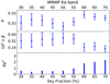 |
Fig. 4. Scaling coefficients for synchrotron and dust (top and middle panels) estimated on different masks for WMAP Ka band. Bottom panel: excess χ2 in units of |


We use the Δχ2 values to select the processing mask to be used in the template fitting. The rule of thumb is to use the mask with the largest fsky among those with Δχ2 ≤ 2. The only exception is represented by WMAP Ka band which shows a sudden change in both scalings, as well an noticeable increase in the excess χ2 between the 55% and 60% masks (see Fig. 4). In this case, we cautiously choose the to use the 55% mask, even though the excess χ2 itself remains slightly below 2 also in the 60% mask. We note how similar jumps between the 55% and 60% masks are evident also in the scalings of the WMAP Q band, shown in Fig. 5. An interesting case is represented by WMAP V band (Fig. 6), for which the Δχ2 reaches a maximum in the 55% mask before decreasing for larger masks, without ever reaching the threshold Δχ2 = 2. In this case we chose the 75% mask. The masks used in the foreground cleaning, together with the scaling coefficients obtained, are reported in Table 3.
Masks used to produce foreground-cleaned maps for each channel, and the corresponding estimates for the scaling coefficients.
The resulting cleaned maps can then be combined together to build inverse-noise-weighted maps. In particular, we build two combinations: the first is a “WMAP-only” map built from the Ka, Q, and V bands, while the second is a joint “WMAP+LFI” map, that uses the Ka, Q, and V WMAP bands and Planck LFI 70 GHz (hereafter WMAP+LFI).
To provide more detail, if  is the final cleaned map of the band, ν, with corresponding noise-covariance matrix,
  , the final noise weighted map, mnw, is built as:
![Mathematical equation: $$ \begin{aligned} \begin{aligned} \mathbf m ^{\mathrm{nw}}&=\left[\sum _{\nu }\left({N}_{\nu }^{P,\mathrm{fc}}\right)^{-1}\right]^{-1}\sum _{\nu }\left({N}_{\nu }^{P,\mathrm{fc}}\right)^{-1}\widetilde{\mathbf{m}}^{P,\mathrm{fc}}_\nu \\&=\overline{\mathcal{N} }\sum _{\nu }\left({N}_{\nu }^{P,\mathrm{fc}}\right)^{-1}\widetilde{\mathbf{m}}^{P,\mathrm{fc}}_\nu \,, \end{aligned} \end{aligned} $$](/articles/aa/full_html/2020/12/aa38508-20/aa38508-20-eq45.gif) (9)
(9)
where we define the total noise covariance matrix:
![Mathematical equation: $$ \begin{aligned} \overline{\mathcal{N} }=\left[\sum _{\nu }\left({N}_{\nu }^{P,\mathrm{fc}}\right)^{-1}\right]^{-1}\,. \end{aligned} $$](/articles/aa/full_html/2020/12/aa38508-20/aa38508-20-eq46.gif) (10)
(10)
We note that in Eq. (9), we use the  with no regularization noise. This is because we do not want to “bring” the regularization noise into the noise-weighted map as we want to avoid possible biases in parameter estimates induced by particular realizations of the regularization noise, as explained in Sect. 4. However, we are forced to use the covariance matrices
  that do include regularization noise since, otherwise, we would not be able to invert them. For this reason, it is evident that
  would be the NCVM of a noise-weighted combination built from the (un-tilded)
  , but is not the NCVM of mnw. The actual NCVM can be computed by rewriting Eq. (9) as
 (11)
(11)
where  denotes the total noise, i.e., the sum of instrumental and regularization noise, at each frequency. Taking the expectation value of mnw(mnw)T yields
![Mathematical equation: $$ \begin{aligned} \begin{aligned}&\langle \mathbf m ^{\mathrm{nw}} (\mathbf m ^{\mathrm{nw}})^{{T}}\rangle \\&={S}+\overline{\mathcal{N} }\sum _{\nu \,\nu^\prime }\left({N}_{\nu }^{P,\mathrm{fc}}\right)^{-1}\langle (\mathbf n ^{t}_\nu -\mathbf n ^{r}_\nu )(\mathbf n ^{t}_{\nu^\prime }-\mathbf n ^{r}_{\nu^\prime })^{T}\rangle \left({N}_{\nu^\prime }^{P,\mathrm{fc}}\right)^{-1}\overline{\mathcal{N} }\\&={S}+\overline{\mathcal{N} }-\left(\sigma ^{{P}}_{{r}}\right)^2\overline{\mathcal{N} }\sum _{\nu }\left[\left({N}_{\nu }^{P,\mathrm{fc}}\right)^{-1}\right]^2\overline{\mathcal{N} }\,, \end{aligned} \end{aligned} $$](/articles/aa/full_html/2020/12/aa38508-20/aa38508-20-eq53.gif) (12)
(12)
where we are assuming that the regularization noise rms  for all the involved maps is the same. In the last equation, we use the fact that
  . Thus, the final noise covariance matrix of the combined instrumental noise is
![Mathematical equation: $$ \begin{aligned} \mathcal{N} \equiv \overline{\mathcal{N} }-\left(\sigma ^{{P}}_{{r}}\right)^2\overline{\mathcal{N} }\sum _{\nu }\left[\left({N}_{\nu }^{P,\mathrm{fc}}\right)^{-1}\right]^2\overline{\mathcal{N} }\,. \end{aligned} $$](/articles/aa/full_html/2020/12/aa38508-20/aa38508-20-eq56.gif) (13)
(13)
6. Power spectra
In this section, we present our results for the angular power spectra of the maps described in the previous sections. In particular, we use a QML code (Tegmark 1996; Tegmark & de Oliveira-Costa 2001) to extract the auto power spectra of the cleaned maps described in Sect. 5. In our analysis, power spectra are not directly used for the cosmological parameter extraction. We mainly use them as a probe of possible residual systematics in the maps and, consequently, for selecting the masks suitable for the likelihood analysis. The main tool for performing these consistency tests is the χ2 in harmonic space, defined as:
 (14)
(14)
where Cℓ is the power spectrum estimated from a given map-and-mask combination,  is the Fisher matrix and
  is the power spectrum of a fiducial ΛCDM model with optical depth of τ = 0.065 and logarithmic amplitude of primordial scalar fluctuations of ln(1010As)=3.0343. We perform separate tests for the TE, TB, EE, EB, and BB power spectra. The quantity in Eq. (14) can be compared to the χ2 distribution with ℓmax − 1 degrees of freedom, computing the corresponding probability-to-exceed (hereafter PTE). In Tables 4–6, we report the PTEs for LFI, WMAP and WMAP+LFI for different sky fractions, corresponding to the masks presented in Sect. 3. As explained in that section, for the WMAP+LFI dataset, the masks are obtained by combining the individual LFI and WMAP masks. We refer the reader to Table 2 for further details.
Probability to exceed  for LFI 70 GHz as a function of the sky fraction.
Probability to exceed  for WMAP as a function of the sky fraction.
Probability to exceed  for the WMAP+LFI dataset as a function of the sky fraction.
Here, we consider 2 ≤ ℓ ≤ 10, which corresponds roughly to the multipole range affected by the reionization feature. For WMAP, the PTEs are nicely compatible with the theoretical model for all the sky fractions considered. For the LFI dataset we see ∼2σ deviations for the BB spectrum for intermediate sky fractions (fsky = 40% and fsky = 45%), fluctuations reabsorbed in larger sky fractions. In the WMAP+LFI dataset, we do not see any particular failure in the PTEs. We define a “failure” as a PTE < 1%.
We further perform additional consistency tests for the combined dataset. We compute the PTEs for different choices of ℓmax, exploring the χ2 consistency up to ℓ = 15 and ℓ = 29. For all the sky fraction we have considered, we do not observe any failure in the total PTEs as a function of ℓmax. We also compute the ℓ-by-ℓ PTEs for all the polarization power spectra. The mask keeping a 54% fraction of the whole sky has the lowest number of outliers above 2.5σ: only 3 out of a total 140 analysed multipoles. As we explain in Sect. 7, the 54% mask also represents a robust choice for the likelihood analysis. The results of the PTEs computation for the combined dataset analysed in the 54% mask are reported in Tables 7 and 8.
Probability to exceed  for the combined dataset WMAP+LFI for different choices of ℓmax.
Probability to exceed  for the WMAP+LFI dataset ℓ-by-ℓ.
The spectra for WMAP, LFI and WMAP+LFI are shown in Fig. 8, in their own 50%, 50%, and 54% masks, respectively.
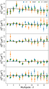 |
Fig. 8. Polarization power spectra of the LFI 70 GHz, WMAP bands and WMAP+LFI. The sky fractions used are respectively 50%, 50%, and 54%. The dashed lines represent a ΛCDM power spectra corresponding to an optical depth value of τ = 0.065. |
7. Likelihood and validation
In this section, we show the results of additional consistency tests performed at the level of parameter estimation. This allows us to test and validate both the datasets produced and the likelihood algorithm.
Parameter estimates are obtained from the likelihood function in Eq. (4). Since we are using low-resolution maps with Nside = 16, only the Cℓ’s from ℓ = 2 to ℓcut = 29 are varied in accordance to the theoretical model that is being tested, when computing the signal covariance matrix; multipoles between ℓcut + 1 = 30 and ℓmax = 64 are instead fixed to a fiducial ΛCDM spectrum (Page et al. 2007; Planck Collaboration XI 2016; Planck Collaboration V 2020). We follow the procedure described in Sect. 4 in order to marginalize over the regularization noise.
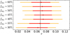 |
Fig. 9. Estimates of τ from the LFI 70 GHz map analysed in different masks. In this and in the following plots, the points represent the best-fit values and the red and yellow bars represent the 68% and 95% C.L., respectively. The vertical grey line represents the best-fit value for the WMAP+LFI baseline dataset, which uses 54% of the sky; see text for details. |
As consistency test for the likelihood, we explore the stability of the reionization optical depth τ constraints with respect the mask used for cosmological parameter estimation. Thus, keeping fixed the underlying datasets (i.e., map and associated covariance matrix) we only change the cosmological parameter mask used in Eq. (4). The results of these test are reported in Figs. 9–11, respectively, for LFI, WMAP and WMAP+LFI. Visually all the τ constraints are nicely compatible with each other for LFI and WMAP. For the WMAP+LFI, the τ posteriors are still visually compatible with each other, but we observe a clear trend towards high values of τ for large sky fractions. It is worth mentioning that all the masks we are using for a given dataset are nested, and largely overlapped, so relying on a simple visual comparison can be misleading and we need a more accurate statistical test to assess consistency. Thus, for each dataset, we generated a Monte Carlo of 1000 CMB maps, with τ = 0.065 and a set of realistic noise simulations extracted from the noise covariance matrix of the cleaned datasets (Eqs. (5) and (13)) through Cholesky decomposition. For every mask, we processed all those maps through a pixel-based likelihood algorithm implementing the function in Eq. (4), fitting τ and ln(1010As) from a grid of models. All the other ΛCDM parameters were kept fixed to the best-fit of Pagano et al. (2020). Then we were able to build the statistics of the difference Δτij ≡ |τi−τj| between the τ estimates for each pair of masks {i, j}, and, finally, compare this with the values of Δτij obtained from the real data
In Table 9, we report the PTEs for the three datasets analyzed, defined as the percentage of simulations that have an absolute parameter shift larger than the same quantity measured on the data. As explained above, the simulations used for this test contain only the CMB signal and noise drawn by cleaned map covariance matrix. We note that foreground residuals and, thus, chance correlations between such residuals and noise realizations are not included in the simulations; this makes the test conservative since it is more difficult to pass. The scatter we see on the data is perfectly compatible with the signal plus noise simulations, independently for LFI and WMAP, and for all the sky fractions considered. The WMAP+LFI dataset, instead, shows mild failures for sky fractions larger than 60%. This comes as some of a surprise since the corresponding results based on WMAP show excellent PTEs (see, e.g., Cols. 2 and 3 of Table 9). Again, we verified that the shift between the Δτ for WMAP and WMAP+LFI are compatible with what is seen in our signal plus noise simulations. We find that all the shifts are within 2σ. This indicates that as far as τ is concerned, all masks return consistent values and may be thus used in the analysis. However, we remark that there is a clear trend towards larger values of τ for masks with a sky fraction larger than fsky = 63% (again, see Fig. 11). Based on these considerations and on the fact that this is the one performing better in the ℓ-by-ℓ tests described in Sect. 6, we opt for a conservative choice and select the 54% mask as the baseline for WMAP+LFI. This dataset provides an error on τ that is 12% smaller than the one obtained from WMAP on the 75% mask.
Consistency of the τ parameter values estimated on different masks.
For the baseline mask, in Table 10, we report the constraints on τ, ln(1010As), both with r = 0 and variable r from the low-multipole dataset alone, having fixed the other ΛCDM parameters to the best-fit of Pagano et al. (2020). In the next section, we offer a detailed discussion on the τ constraints and its consequences for the cosmological scenario.
Constraints on ln(1010As), τ, and r from the WMAP+LFI likelihood.
8. Reionization constraints
The CMB large-scale polarization data provide an almost direct measurement of the optical depth to reionization, being  and
and  for multipoles ℓ ≲ 20. In this section, we use the WMAP+LFI dataset in polarization, together with the Commander 2018 solution in temperature, to derive updated constraints on τ from CMB measurements at low frequencies.
For the cosmological parameter tests presented in this paper, we adopted the reionization model given in Lewis (2008). This is the default model in camb4 and it has been used for the Planck baseline cosmological results (TANH). In this model, the phase change in the intergalactic medium from the almost completely neutral state (up to a residual ionization fraction of 10−4, remaining after recombination) to the ionized state is described as a sharp transition. The hydrogen reionization is assumed to happen simultaneously with the first reionization of helium, whereas the second reionization of helium is fixed at a redshift of z = 3.5 and is, again, described as a sharp transition. This choice is motivated by the expectations drawn from quasar spectra. Nevertheless, we expect the modeling of the helium double ionization to have a minor impact on the final results because varying the corresponding reionization redshift between 2.5 and 4.5 changes the total optical depth by less than 1% (Planck Collaboration Int. XLVII 2016). For the tests presented in this paper, we did not explore different reionization models, however, it has been shown in Planck Collaboration VI (2020) that τ constraints from the latest Planck data have little sensitivity with regard to the actual details of the reionization history. Furthermore, earlier claims by Heinrich & Hu (2018) of a mild evidence, in Planck 2015 LFI data, for a more complex model of the ionization fraction, with hints of early reionization, have not been confirmed by alternate analyses of the same data set (e.g., Villanueva-Domingo et al. 2018; Hazra & Smoot 2017; Dai et al. 2019; Hazra et al. 2020). In particular, Millea & Bouchet (2018) have shown how the significance of those findings has been likely overestimated due to the choice of unphysical priors.
Having fixed the reionization model, first of all, we want to study the constraints from the large scales alone. Using the pixel-based likelihood framework of Sect. 7 (lowTEB), we only fit for τ, ln(1010As), and r, while keeping all the other ΛCDM parameters fixed to the best-fit values given in Pagano et al. (2020). Our results are shown in Table 10, where the parameter, r, is estimated at a scale of k = 0.002 Mpc−1. The derived constraint on τ is
 (15)
(15)
which corresponds to a 5.8σ detection from the low-frequency CMB polarization data.
We then extended the analysis to include data from the small scales, specifically adding the Planck 2018 likelihood for TT, TE, EE angular power spectra (Planck Collaboration V 2020). This time, we let all the six base ΛCDM parameters vary, and we sampled from the space of possible cosmological parameters with an MCMC exploration using CosmoMC (Lewis & Bridle 2002). The reionization optical depth estimated in this case is5:
 (16)
(16)
The parameter constraints we derived for pure ΛCDM are given in Table 11, where, for the purposes of comparison, we also report the Planck 2018 baseline results. The two compared datasets differ by the low-ℓ likelihoods. In one case, there is the pixel-based likelihood developed in this paper (lowTEB), while in the other case, the low-ℓ likelihood is a combination of the Blackwell-Rao estimator for the Commander temperature solution and the E-mode power spectrum based Planck Legacy HFI likelihood (lowE). The latter likelihood provides a constraint on τ that is about 1.5 times tighter and 1.4σ lower in value than the one we obtain from the WMAP+LFI likelihood. Due to the well known degeneracy between As and τ, this also translates to a 33% tighter constraint on ln(1010As) and 1.8σ lower in value. All the other cosmological parameters, rather, are in good agreement, differing by at most 36% of the σ. A similar tendency is also found when comparing Table 11 with an analogous analysis shown in Pagano et al. (2020).
Parameter constraints for the ΛCDM cosmology (as defined in Planck Collaboration XVI 2014), illustrating the impact of replacing the low-ℓ baseline Planck 2018 likelihood (lowE) with the WMAP+LFI likelihood presented in this paper (lowTEB).
Comparing the constraints from Tables 10 and 11, we note that the values of ln(1010As) and τ derived from the large scales alone are 1.9σ and 0.4σ lower, respectively. This behaviour was first noticed in Planck Collaboration XI (2016) and it is known to be induced by the low-ℓ anomaly, that is, the power deficit in the measured TT power spectrum with respect to the best-fit model at multipoles between ℓ = 20 and 30. When limiting the analysis to the large scales, that is, to multipoles up to 30, the deficit has a high relative weight in the final solution, leading to a value of the overall amplitude of the spectrum that is lower than the one from the full analysis, which includes multipoles up to ℓ = 2500. Due to the aforementioned degeneracy, this also results in a lower value for τ.
Since one of the main results of this paper is the τ constraint from the WMAP+LFI dataset, we want to further comment on the robustness of this result. In Fig. 12, we show the good agreement between the estimates of τ from LFI and WMAP separately. The two were derived using their own fsky = 50% mask. The consistency between the two experiments is further confirmed by the null test that we performed, estimating τ from the half-difference map of the two data sets, LFI−WMAP. The posterior distribution for this case is reported in the same figure and it is compatible with noise, giving an upper limit of τ ≤ 0.059 at 95% confidence level (CL).
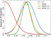 |
Fig. 12. Posterior distributions of τ. LFI (blue) and WMAP (orange) are computed on their own 50% mask, WMAP+LFI (green) in the union of the two, retaining 54% of the sky, while WMAP−LFI (red) is computed in their intersection, retaining 46% of the sky. |
Differently from the baseline low-ℓ Planck 2018 likelihood, which is based on the TT, EE, and BB power spectra, the pixel-based likelihood used in this paper also includes the information contained in the TE cross power spectrum. In order to investigate the impact of this extra information, we build a polarization-only version of the pixel-based likelihood, which contains only the Q and U maps and the QQ, QU, and UU blocks of the covariance matrix, in an analogy of what was done in Planck Collaboration XI (2016). When we use this latter likelihood, we employ low-ℓ TTCommander likelihood based on the Blackwell-Rao estimator. The value of τ measured nulling the TE cross correlation is
 (17)
(17)
which represents roughly a half-σ downward shift with respect to the full TEB likelihood, already seen on the LFI only likelihood in Planck Collaboration XI (2016). Such behavior is also shown by WMAP which, on 50% sky, yields  forcing TE = 0 and
  with the full TEB likelihood. For WMAP, the same behavior is also present on larger masks; for example on the 75% sky fraction we measure
  when TE = 0 and
  when also TE is varied.
In all the previous cases, when TE is forced to zero, the τ posterior shifts closer to the HFI determination (Planck Collaboration V 2020; Pagano et al. 2020), which is based only on EE estimates. Posteriors of the full pixel-based likelihood and the one without TE for WMAP+LFI are shown in Fig. 13.
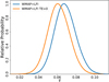 |
Fig. 13. Comparison of τ posterior distributions for the WMAP+LFI using the full TQU likelihood (blue) and imposing TE = 0 in order to factorize the T and QU parts of the likelihood (orange). |
In order to verify if such behaviour is coherent with our error budget, we compare the shift in τ with a set of simulations. In Fig. 14 we show the histogram of Δτ, defined as the difference between the τ estimated form the full TEB likelihood (“Full”) and the τ estimated forcing TE = 0 (“noTE”), for a Montecarlo of 1000 signal and noise simulations. This analysis shows that nullifying TE still provides an unbiased estimation of τ and also that the shift observed in data is not anomalous, representing a 1.7σ fluctuation. We also show in Fig. 15, a similar plot for the ratio of 1σ errors defined as στnoTE/στFull; also, in this case, the value measured on data is compatible with the simulations. This test also suggests that for this dataset, removing TE degrades στ by about 5% on average.
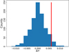 |
Fig. 14. Histogram of Δτ ≡ τFull − τnoTE obtained analyzing a Montecarlo of 1000 simulations. The red vertical bar shows the same quantity evaluated on the data. |
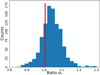 |
Fig. 15. Histogram of στnoTE/στFull obtained analyzing a Montecarlo of 1000 simulations. The red vertical bar shows the same quantity evaluated on the data. |
Adding to the CMB temperature and polarization data the Planck lensing likelihood (Planck Collaboration VIII 2020) and baryon acoustic oscillation (BAO) measurements (Alam et al. 2017; Beutler et al. 2011; Ross et al. 2015) breaks the degeneracy more efficiently with the amplitude of the scalar perturbations providing
 (18)
(18)
Assuming the TANH model for the ionzation fraction the τ constrain can be directly converted into a mid-point reionization redshift of
 (19)
(19)
This value is higher but still compatible with analogous estimates that instead use the Planck HFI based large-scale polarization likelihood, zre = 7.82 ± 0.71 (Planck Collaboration VI 2020) and zre = 8.21 ± 0.58 (Pagano et al. 2020).
The WMAP+LFI CMB map and the corresponding covariance matrix are packaged in low-ℓ likelihood modules compatible with the clik infrastructure (Planck Collaboration XV 2014; Planck Collaboration ES 2013, 2015, 2018) which are made publicly available6. We provide both a likelihood module that implements Eq. (4) inverting the full covariance matrix and one that implements the Sherman-Morrison-Woodbury (SMW) formula (Golub & Van Loan 1996) which allows us to speed up the computation by an order of magnitude (see Planck Collaboration XI 2016, Appendix B.1 for details) but does not include TB an EB. In both cases, in order to keep full compatibility with the codes of clik framework, we do not treat the regularization noise as described in Sect. 4, but instead we sum a single realization. Such noise realization has been chosen in order to have a deviation for ln(1010As) and τ with respect to the baseline case smaller than 1% in units of σ.
9. Conclusions
In this work, we present a novel CMB pixel-space likelihood focussed on polarization at large angular scales, whose main cosmological target is the optical depth to reionization, τ. The underlying dataset combines foreground-mitigated WMAP Ka, Q, and V bands with Planck LFI 70 GHz channel in an optimally weighted CMB map. In the foreground cleaning of WMAP bands, we adopt the Planck 353 GHz channel as a dust template, instead of the WMAP dust model based on starlight-derived polarization directions. As a synchrotron template, the K band is used for WMAP channels, while Planck 30 GHz is used for the 70 GHz map. The corresponding covariance matrix is computed coherently and fed, together with the cleaned CMB map, into a pixel space likelihood, made publicly available with this paper. We produced a set of masks with increasing sky fraction and used them to test the performance of the component separation, the quality of polarization power spectra, and the overall stability of τ constraints, showing a remarkable stability among sky fractions.
For the baseline dataset, which retains 54% of the sky, the ℓ-by-ℓ probability to exceed the χ2 of the measured angular power spectra (PTE) does not show any major outlier, with only ℓ = 18 and 23 of BB and ℓ = 23 of EB spectra at more than 2.5σ. Consequently, the integrated PTEs are perfectly consistent with simulations both on the reionization peak only (i.e., ℓ = 2 ÷ 10) and on the full multipole range (i.e., ℓ = 2 ÷ 29).
Regarding the reionization optical depth estimation, we compared the variation of τ estimated on different sky fractions with a Montecarlo of signal plus noise, finding no significant deviations for the baseline dataset compared with other sky fractions, up to fsky ∼ 70%.
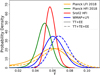 |
Fig. 16. Posterior distributions for τ for various datasets. Solid lines represent τ constraints ignoring TE, dashed lines assume full TEB likelihood. Only τ and ln(1010As) are sampled, whereas the remaining ΛCDM parameters are fixed to common fiducial values. The green and yellow lines show results obtained with the official Planck Legacy low-ℓ likelihoods (Planck Collaboration V 2020). The red line is obtained running the SRoll2 likelihood (Pagano et al. 2020). The blue lines represent the results of this paper. |
Sampling the parameter space with our low-ℓ likelihood only, we find  . When CMB small scales, BAO observations, and Planck lensing likelihood are included, we shrink optical depth constraint down to
  . Such bounds are slightly less constraining when compared with the existing Planck HFI based likelihood (see, e.g., Planck Collaboration V 2020; Pagano et al. 2020, and our Fig. 16), yet they represent a novel measurement obtained with an independent pipeline that adopts different data and likelihood approximation and includes TE correlation, while the Planck HFI estimates are currently restricted to EE information. The τ estimates obtained with the likelihood package discussed in this paper is, in general, very compatible with the Planck HFI based constraints, with a preference for slightly higher τ values, probably driven by the inclusion of TE. This bound is also in perfect agreement with the Planck LFI Legacy likelihood (Planck Collaboration V 2020). Within the ΛCDM model, τ can be also constrained without the use of polarization data to break the degeneracy between As and τ, combining temperature and weak lensing data. In this kind of analysis, the Planck collaboration found τ = 0.080 ± 0.025 from temperature and lensing data and τ = 0.078 ± 0.016 when BAO is added (Planck Collaboration ES 2018). Those values, despite being slightly higher than previous findings (Weiland et al. 2018; Planck Collaboration XIII 2016), are still in agreement with our constraints.
The likelihood package we provide is built on a real-space estimator and does not assume rotational invariance, but, rather, only the Gaussianity of the fields, which secures several advantages. For instance, it can also be easily used for constraining non-rotationally invariant cosmologies, including, naturally, the TB and EB spectra in the parameter exploration.
Here “fc” stands for “foreground-cleaned”.
In the following, the presence of the lowTEB dataset should be always understood.
The WMAP+LFI likelihood module is available on https://web.fe.infn.it/~pagano/low_ell_datasets/wmap_lfi_legacy
Acknowledgments
We acknowledge the use of camb, HEALPix and Healpy software packages, and the use of computing facilities at CINECA. We are grateful to M. Gerbino for useful suggestions. MM is supported by the program for young researchers “Rita Levi Montalcini” year 2015. We acknowledge support from the COSMOS network (www.cosmosnet.it) through the ASI (Italian Space Agency) Grants 2016-24-H.0 and 2016-24-H.1-2018.
References
- Alam, S., Ata, M., Bailey, S., et al. 2017, MNRAS, 470, 2617 [NASA ADS] [CrossRef] [Google Scholar]
- Benabed, K., Cardoso, J. F., Prunet, S., & Hivon, E. 2009, MNRAS, 400, 219 [NASA ADS] [CrossRef] [Google Scholar]
- Bennett, C. L., Larson, D., Weiland, J. L., et al. 2013, ApJS, 208, 20 [Google Scholar]
- Beutler, F., Blake, C., Colless, M., et al. 2011, MNRAS, 416, 3017 [NASA ADS] [CrossRef] [Google Scholar]
- Dai, W.-M., Ma, Y.-Z., Guo, Z.-K., & Cai, R.-G. 2019, Phys. Rev. D, 99, 043524 [CrossRef] [Google Scholar]
- Delouis, J. M., Pagano, L., Mottet, S., Puget, J. L., & Vibert, L. 2019, A&A, 629, A38 [NASA ADS] [CrossRef] [EDP Sciences] [Google Scholar]
- Gerbino, M., Lattanzi, M., Migliaccio, M., et al. 2020, Front. Phys., 8, 15 [CrossRef] [Google Scholar]
- Golub, G. H., & Van Loan, C. F. 1996, Matrix Computations, 3rd edn. (The Johns Hopkins University Press) [Google Scholar]
- Górski, K. M., Hivon, E., Banday, A. J., et al. 2005, ApJ, 622, 759 [NASA ADS] [CrossRef] [Google Scholar]
- Hazra, D. K., & Smoot, G. F. 2017, JCAP, 1711, 028 [NASA ADS] [CrossRef] [Google Scholar]
- Hazra, D. K., Paoletti, D., Finelli, F., & Smoot, G. F. 2020, Phys. Rev. Lett., 125, 071301 [CrossRef] [Google Scholar]
- Heinrich, C., & Hu, W. 2018, Phys. Rev. D, 98, 063514 [CrossRef] [Google Scholar]
- Hinshaw, G., Larson, D., Komatsu, E., et al. 2013, ApJS, 208, 19 [NASA ADS] [CrossRef] [Google Scholar]
- Lattanzi, M., Burigana, C., Gerbino, M., et al. 2017, JCAP, 1702, 041 [NASA ADS] [CrossRef] [Google Scholar]
- Lewis, A. 2008, Phys. Rev. D, 78, 023002 [NASA ADS] [CrossRef] [Google Scholar]
- Lewis, A., & Bridle, S. 2002, Phys. Rev. D, 66, 103511 [NASA ADS] [CrossRef] [Google Scholar]
- Millea, M., & Bouchet, F. 2018, A&A, 617, A96 [CrossRef] [EDP Sciences] [Google Scholar]
- Pagano, L., Delouis, J.-M., Mottet, S., Puget, J.-L., & Vibert, L. 2020, A&A, 635, A99 [CrossRef] [EDP Sciences] [Google Scholar]
- Page, L., Hinshaw, G., Komatsu, E., et al. 2007, ApJS, 170, 335 [NASA ADS] [CrossRef] [Google Scholar]
- Planck Collaboration ES 2013, The Explanatory Supplement to the Planck 2013 Results (ESA), https://www.cosmos.esa.int/web/planck/pla [Google Scholar]
- Planck Collaboration ES 2015, The Explanatory Supplement to the Panck 2015 Results (ESA) [Google Scholar]
- Planck Collaboration ES 2018, The Legacy Explanatory Supplement (ESA), https://www.cosmos.esa.int/web/planck/pla [Google Scholar]
- Planck Collaboration XV. 2014, A&A, 571, A15 [NASA ADS] [CrossRef] [EDP Sciences] [Google Scholar]
- Planck Collaboration XVI. 2014, A&A, 571, A16 [NASA ADS] [CrossRef] [EDP Sciences] [Google Scholar]
- Planck Collaboration XXIII. 2014, A&A, 571, A23 [NASA ADS] [CrossRef] [EDP Sciences] [MathSciNet] [PubMed] [Google Scholar]
- Planck Collaboration XI. 2016, A&A, 594, A11 [NASA ADS] [CrossRef] [EDP Sciences] [Google Scholar]
- Planck Collaboration XIII. 2016, A&A, 594, A13 [NASA ADS] [CrossRef] [EDP Sciences] [Google Scholar]
- Planck Collaboration XVI. 2016, A&A, 594, A16 [NASA ADS] [CrossRef] [EDP Sciences] [Google Scholar]
- Planck Collaboration I. 2020, A&A, 641, A1 [CrossRef] [EDP Sciences] [Google Scholar]
- Planck Collaboration II. 2020, A&A, 641, A2 [CrossRef] [EDP Sciences] [Google Scholar]
- Planck Collaboration III. 2020, A&A, 641, A3 [NASA ADS] [CrossRef] [EDP Sciences] [Google Scholar]
- Planck Collaboration IV. 2020, A&A, 641, A4 [CrossRef] [EDP Sciences] [Google Scholar]
- Planck Collaboration V. 2020, A&A, 641, A5 [CrossRef] [EDP Sciences] [Google Scholar]
- Planck Collaboration VI. 2020, A&A, 641, A6 [NASA ADS] [CrossRef] [EDP Sciences] [Google Scholar]
- Planck Collaboration VIII. 2020, A&A, 641, A8 [CrossRef] [EDP Sciences] [Google Scholar]
- Planck Collaboration Int. XLVII. 2016, A&A, 596, A108 [NASA ADS] [CrossRef] [EDP Sciences] [Google Scholar]
- Ross, A. J., Samushia, L., Howlett, C., et al. 2015, MNRAS, 449, 835 [NASA ADS] [CrossRef] [Google Scholar]
- Tegmark, M. 1996, MNRAS, 280, 299 [NASA ADS] [CrossRef] [Google Scholar]
- Tegmark, M., & de Oliveira-Costa, A. 2001, Phys. Rev. D, 64, 063001 [NASA ADS] [CrossRef] [Google Scholar]
- Villanueva-Domingo, P., Gariazzo, S., Gnedin, N. Y., & Mena, O. 2018, JCAP, 1804, 024 [NASA ADS] [CrossRef] [Google Scholar]
- Weiland, J., Osumi, K., Addison, G., et al. 2018, ApJ, 863, 161 [NASA ADS] [CrossRef] [Google Scholar]
All Tables
Foreground scalings coefficients from WMAP K-band (α) and Planck 353 GHz (β) to the indicated WMAP channels.
Masks used to produce foreground-cleaned maps for each channel, and the corresponding estimates for the scaling coefficients.
Probability to exceed for the WMAP+LFI dataset as a function of the sky fraction.
Probability to exceed for the combined dataset WMAP+LFI for different choices of ℓmax.
Parameter constraints for the ΛCDM cosmology (as defined in Planck Collaboration XVI 2014), illustrating the impact of replacing the low-ℓ baseline Planck 2018 likelihood (lowE) with the WMAP+LFI likelihood presented in this paper (lowTEB).
All Figures
|
Fig. 1. Subset of the masks used in the analysis of the LFI 70 GHz data. Values of the available sky fraction fsky in each mask are 30%, 40%, 50%, and 60%. |
| In the text | |
|
Fig. 2. Subset of the masks used in the analysis of the WMAP data. Values of the available sky fraction fsky in each mask are 30%, 40%, 50%, and 60%. |
| In the text | |
|
Fig. 3. Histograms of the expected scatter in the recovered foreground scalings, in the χ2 of the component separation and in the measured τ due to the regularization noise. For each quantity, we show the distance from the center of the empirical distribution in units of σ. |
| In the text | |
|
Fig. 4. Scaling coefficients for synchrotron and dust (top and middle panels) estimated on different masks for WMAP Ka band. Bottom panel: excess χ2 in units of |
| In the text | |
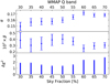 |
Fig. 5. Same as Fig. 4, but for the WMAP Q band. |
| In the text | |
 |
Fig. 6. Same as Fig. 4, but for the WMAP V band. |
| In the text | |
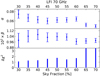 |
Fig. 7. Same as Fig. 4, but for the Planck LFI 70 GHz channel. |
| In the text | |
|
Fig. 8. Polarization power spectra of the LFI 70 GHz, WMAP bands and WMAP+LFI. The sky fractions used are respectively 50%, 50%, and 54%. The dashed lines represent a ΛCDM power spectra corresponding to an optical depth value of τ = 0.065. |
| In the text | |
|
Fig. 9. Estimates of τ from the LFI 70 GHz map analysed in different masks. In this and in the following plots, the points represent the best-fit values and the red and yellow bars represent the 68% and 95% C.L., respectively. The vertical grey line represents the best-fit value for the WMAP+LFI baseline dataset, which uses 54% of the sky; see text for details. |
| In the text | |
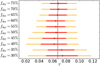 |
Fig. 10. Same as Fig. 9 but for the combination of WMAP Ka, Q and V bands. |
| In the text | |
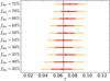 |
Fig. 11. Same as Fig. 9 but for the WMAP+LFI dataset. |
| In the text | |
|
Fig. 12. Posterior distributions of τ. LFI (blue) and WMAP (orange) are computed on their own 50% mask, WMAP+LFI (green) in the union of the two, retaining 54% of the sky, while WMAP−LFI (red) is computed in their intersection, retaining 46% of the sky. |
| In the text | |
|
Fig. 13. Comparison of τ posterior distributions for the WMAP+LFI using the full TQU likelihood (blue) and imposing TE = 0 in order to factorize the T and QU parts of the likelihood (orange). |
| In the text | |
|
Fig. 14. Histogram of Δτ ≡ τFull − τnoTE obtained analyzing a Montecarlo of 1000 simulations. The red vertical bar shows the same quantity evaluated on the data. |
| In the text | |
|
Fig. 15. Histogram of στnoTE/στFull obtained analyzing a Montecarlo of 1000 simulations. The red vertical bar shows the same quantity evaluated on the data. |
| In the text | |
|
Fig. 16. Posterior distributions for τ for various datasets. Solid lines represent τ constraints ignoring TE, dashed lines assume full TEB likelihood. Only τ and ln(1010As) are sampled, whereas the remaining ΛCDM parameters are fixed to common fiducial values. The green and yellow lines show results obtained with the official Planck Legacy low-ℓ likelihoods (Planck Collaboration V 2020). The red line is obtained running the SRoll2 likelihood (Pagano et al. 2020). The blue lines represent the results of this paper. |
| In the text | |
Current usage metrics show cumulative count of Article Views (full-text article views including HTML views, PDF and ePub downloads, according to the available data) and Abstracts Views on Vision4Press platform.
Data correspond to usage on the plateform after 2015. The current usage metrics is available 48-96 hours after online publication and is updated daily on week days.
Initial download of the metrics may take a while.