| Issue |
A&A
Volume 643, November 2020
|
|
|---|---|---|
| Article Number | A15 | |
| Number of page(s) | 7 | |
| Section | Galactic structure, stellar clusters and populations | |
| DOI | https://doi.org/10.1051/0004-6361/202039012 | |
| Published online | 27 October 2020 | |
The elusive tidal tails of the Milky Way globular cluster NGC 7099⋆
1
Instituto Interdisciplinario de Ciencias Básicas (ICB), CONICET-UNCUYO, Padre J. Contreras 1300, M5502JMA Mendoza, Argentina
e-mail: andres.piatti@unc.edu.ar
2
Consejo Nacional de Investigaciones Científicas y Técnicas (CONICET), Godoy Cruz 2290, C1425FQB Buenos Aires, Argentina
3
Instituto de Alta Investigación, Universidad de Tarapacá, Casilla 7D, Arica, Chile
4
Instituto de Astrofísica, Facultad de Física, Pontificia Universidad Católica de Chile, Av. Vicuña Mackenna 4860, 782-0436 Macul, Santiago, Chile
5
European Southern Observatory, Alonso de Córdova 3107, Casilla 19001 Santiago, Chile
6
Millenium Institute of Astrophysics, Santiago, Chile
Received:
23
July
2020
Accepted:
8
September
2020
We present results on the extra-tidal features of the Milky Way globular cluster NGC 7099, using deep gr photometry obtained with the Dark Energy Camera (DECam). We reached nearly 6 mag below the cluster’s main sequence (MS) turnoff, so that we dealt with the most suitable candidates to trace any stellar structure located beyond the cluster tidal radius. From star-by-star reddening corrected color-magnitude diagrams (CMDs), we defined four adjacent strips along the MS, for which we built the respective stellar density maps, once the contamination by field stars was properly removed. The resulting, cleaned, field star stellar density maps show a short tidal tail and some scattered debris. Such extra-tidal features are hardly detected when much shallower Gaia DR2 data sets are used and the same CMD field star cleaning procedure is applied. Indeed, by using 2.5 mag below the MS turnoff of the cluster as the faintest limit (G < 20.5 mag), cluster members turned out to be distributed within the cluster’s tidal radius, and some hints for field star density variations are found across a circle of radius 3.5° centered on the cluster and with similar CMD features as cluster stars. The proper motion distribution of these stars is distinguishable from that of the cluster, with some superposition, which resembles that of stars located beyond 3.5° from the cluster center.
Key words: methods: observational / techniques: photometric
DECam photometric data are only available at the CDS via anonymous ftp to cdsarc.u-strasbg.fr (130.79.128.5) or via http://cdsarc.u-strasbg.fr/viz-bin/cat/J/A+A/643/A15
© ESO 2020
1. Introduction
Tidal streams are witnesses of accreted dwarf galaxies that are disrupted by the Milky Way. They have been unveiled from wide-sky photometric and spectroscopic surveys, including the Sloan Digital Sky Survey (SDSS)1, the Two Micron All-Sky Survey (2MASS)2, the Panoramic Survey Telescope and Rapid Response System (Pan-STARRS)3, the Dark Energy Survey (DES)4, and the Gaia mission5. The most spectacular example of these stellar substructures in the Milky Way halo is the one generated by the assimilation of the Sagittarius dwarf galaxy, which is moving around the Milky Way in an almost polar orbit (Ibata et al. 1994; Majewski et al. 2003; Belokurov et al. 2006; Koposov et al. 2012). Additional well-known streams in the Milky Way include the Monoceros ring, which may represent an on-plane accretion of a minor satellite, and the Sausage-Enceladus structure, which was recently discovered in the Gaia DR2 (Belokurov et al. 2018; Helmi et al. 2018) and it seems to be associated with the impact of an Small Magellanic Cloud-like mass galaxy on the Milky Way. There are also minor streams that have been reported by Mateu et al. (2018) as well as newly identified streams by Ibata et al. (2018).
Out of a family of ∼160 Galactic globular clusters, nearly 50 have been associated with one (or several) of the accreted galaxies and tidal streams discovered so far in the halo, based on their projected positions, kinematics, and chemical abundances (Bellazzini et al. 2003; Forbes & Bridges 2010; Massari et al. 2019). However, the unambiguous confirmation of the extra-Galactic origin of one of the halo globular clusters requires the combination of multiple techniques and an important observational effort (see Carballo-Bello et al. 2017), so that most of the globular clusters on that list remain candidates.
It has been thought that the structure of Milky Way globular clusters might provide precious information about their origin and accretion processes as well as about the internal dynamical evolution of the cluster. Interestingly, many of the hypothetically accreted halo globular clusters show the signature of the presence of extra-tidal stars in the form of tidal tails (e.g., Pal 5, Odenkirchen et al. 2003) and extended halos (e.g., 47 Tuc, Piatti 2017a). For instance, in the case of the Sausage-Enceladus accretion event, most of the associated globular clusters proposed by Myeong et al. (2018) are embedded in a stellar component, which is only revealed using matched-filter techniques on deep wide-field photometry (Carballo-Bello et al. 2014, 2018; Vanderbeke et al. 2015; Kuzma et al. 2016; Carballo-Bello 2019; Piatti & Carballo-Bello 2019). One of the open questions in the study of the Milky Way’s globular clusters is whether the outer structure of a globular cluster is defined by its formation conditions within a smaller protogalactic fragment or whether it is exclusively defined by its internal evolution and the orbit that followed around the Milky Way (Massari et al. 2019; Piatti & Carballo-Bello 2020).
In this study, we focus on NGC 7099, which is a poorly studied Milky Way globular cluster that might have formed within the Sausage-Enceladus galaxy (Massari et al. 2019). With peri- and apogalactocentric distances of 1.49 kpc and 8.15 kpc, respectively (Baumgardt et al. 2019), NGC 7099 moves along its retrograde orbit with a relatively high eccentricity and inclination angle (e = 0.69, i = 61.5°, Piatti 2019), so it could have crossed the inner disk regions many times. NGC 7099 has lost ∼30% of its initial mass by tidal heating caused by the Milky Way’s gravitational field, in addition to another half of its initial mass by stellar evolution (Piatti et al. 2019). In Sect. 2, we describe the observational data collected, on which our analysis relies. Sections 2 and 3 detail the cleaning procedure applied to the observed NGC 7099 color-magnitude diagram (CMD), which was used to get rid of the field star contamination and build the respective stellar density maps. Additionally, we discuss our results in light of recent findings (Sollima 2020, hereafter S20).
2. Data collection and processing
In this work we have used the Dark Energy Camera (DECam), which is mounted at the prime focus of the 4 m Blanco telescope at Cerro Tololo Inter-American Observatory (CTIO). DECam provides a 3 deg2 field of view with its 62 identical chips with a scale of 0.263 arcsec pixel−1 (Flaugher et al. 2015). NGC 7099 was included among the targets of the observing program 2019B-1003 (08/09.08.2019) and the exposure times were 600 × 4 s and 600 × 4 s, for the g and r bands, respectively. We also observed 3–5 SDSS fields per night at a different airmass to derive the atmospheric extinction coefficients and the transformations between the instrumental magnitudes and the SDSS ugriz system (Fukugita et al. 1996).
The images were processed by the DECam Community Pipeline (Valdes et al. 2014) and accessed via the NOAO Science Archive. The photometry was obtained from the images with the PSF-fitting algorithm of DAOPHOT II/ALLSTAR (Stetson 1987). The final catalog only includes stellar-shaped objects with |sharpness| ≤ 0.5 to avoid, as much as possible, the presence of background galaxies and nonstellar sources in our analysis.
We also used DAOPHOT II to include synthetic stars in our images in order to estimate the completeness of our photometric catalogs. After applying our photometry pipeline, the limiting magnitude was set at the magnitude at which the synthetic stars are only recovered in 50% of the altered images. For g and r bands, the limiting magnitudes in our catalogs are 23.4 mag and 23.3 mag, respectively.
We retrieved the E(B − V) values as a function of RA and Dec from Schlafly & Finkbeiner (2011) provided by the NASA/IPAC Infrared Science Archive6 for the entire analyzed area. Figure 1 shows that the interstellar extinction along the line-of-sight is low, with a maximum difference between the most and least reddened regions of ≲0.02 mag. Using Fig. 1, we assigned individual E(B − V) values to the measured stars according to their positions in the sky. In order to correct the observed magnitudes and colors by interstellar extinction, we used the individual E(B − V) values and the Aλ/AV coefficients given by Wang & Chen (2019). With the aim of illustrating the wealth of information we gathered, Fig. 2 depicts the intrinsic CMD of the inner cluster region (r < 0.15°) and that of a sky annular region centered on the cluster with an equivalent area and external radius of 0.8°. By comparing both panels of Fig. 2, we conclude that the NGC 7099 CMD is affected by a low field contamination. Figure 2 also reveals a relatively narrow MS of the cluster, which extends more than 5 mag in g.
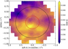 |
Fig. 1. Reddening map across the field of NGC 7099. The red and black circles are of 0.32° and 0.73° in radius, respectively. The black circle separates two areas of the same size. |
3. Stellar density maps
Because of two-body relaxation, less massive stars are candidates to escape the cluster more easily than more massive ones (Balbinot & Gieles 2018). Hence, fainter cluster main sequence (MS) stars are usually used to search for extra-tidal structures around globular clusters (see Piatti & Fernández-Trincado 2020, and references therein). We, therefore, take advantage of the well-delineated MS shown in Fig. 2 to define four adjacent strips, from underneath the MS turnoff down to 4 mag below it, to map the distribution of their stellar populations. The stellar density map of the cluster is then constructed in a straightforward manner for the four different subsets of MS stars of the cluster.
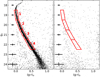 |
Fig. 2. CMDs of stars in the field of NGC 7099 (r < 0.15°; left panel) and in an annular region of the same area centered on the cluster with an external radius of 0.8° (right panel). The four regions along the MS of the cluster that were used to perform star counts are delineated with red contour lines. |
Figure 3 shows the stellar density maps built for each MS strip using the AstroML (VanderPlas et al. 2012) kernel density estimator (KDE) routine. We superimposed a grid of 100 × 100 square cells onto the area of interest (r < 0.73°) and used a range of values for the KDE bandwidth from 0.02° up to 0.07° in steps of 0.01° in order to apply the KDE to each generated cell. We adopted a bandwidth of 0.05° as the optimal value. We also estimated the background level using the stars distributed within the annular region, which is defined by the black circle in Fig. 1, and an external radius of 0.8°. We divided this type of annulus into 16 adjacent sectors of 22.5° wide and counted the number of stars inside them. We rotated such an array of sectors by 11.25° and repeated the star counting. Finally, we derived the mean value in the 32 defined sectors, which turned out to be 35.5, 133.3, 114.0, and 100.0 stars deg−2 for the MS strips #1 to 4, respectively. As for the standard deviation, we performed a thousand Monte Carlo realizations using the stars located beyond the red circle in Fig. 1, which were rotated randomly (one different angle for each star) before recomputing the density map. The resulting standard deviation of all the generated density maps turned out to be 20.3, 47.7, 41.4, and 44.6 stars deg−2 for the MS strips #1 to 4, respectively. The color scale in Fig. 3 represents the absolute deviation from the mean value in the field in units of the standard deviation, that is, η = (signal − mean value)/standard deviation. We have painted white stellar densities with η > 10 in order to highlight the least dense structures. The same Monte Carlo procedure described above has been employed to determine the background density and its standard deviation in the cleaned CMD has been used to calculate the value of η.
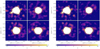 |
Fig. 3. Observed (left panels) and field star cleaned (right panels) stellar density maps for the four MS strips of the cluster of Fig. 2 as labeled at the top-left margin of each panel. The black circle centered on the cluster indicates the assumed tidal radius. Contours for η = 1, 2, 4, 6, 8, and 10 are also shown; the colors follow the coding shown at the bottom of each panel. |
We applied a procedure to get rid of field stars that fall inside the four defined MS strips. The method was devised by Piatti & Bica (2012) and it was satisfactory in cleaning CMDs of star clusters projected toward crowded star fields (e.g., Piatti 2017b,c,a, and references therein) and affected by differential reddening (e.g., Piatti 2018; Piatti et al. 2018, and references therein). The method uses the magnitudes and colors of stars in a reference field CMD to subtract an equal number of stars in the cluster CMD that best resembles the reference field CMD. This is done by considering the position of each field star in the cluster CMD and by subtracting the closest star in the cluster CMD to that field star. The star-to-star subtraction in the cluster CMD is necessary to avoid stochastic effects and subtraction residuals, which arise when any fixed size for boxes homogeneously distributed throughout the CMD is chosen to count stars into them. We thus tightly reproduce the reference field CMD in terms of luminosity function, color distribution, and stellar density. The purpose of this type of cleaning is to obtain a cluster CMD without field contamination. The contribution of field stars is included in the observed stellar density maps. The cleaning procedure subtracts the exact number of field stars that contribute to the reference field CMD. The procedure searches throughout the whole cluster area for field stars to eliminate, giving the same chance (weight) to every subregion to contain such a field star. This is done to avoid spurious overdensities in the cleaned cluster field. If the star field were homogeneous and contained N stars per unit area, the procedure would subtract N stars per unit area. If there were any intrinsic spatial gradient of field stars in the cluster area, the procedure would eliminate it, at the expense of leaving some residuals as a counterpart of the excess of stars subtracted from the inner cluster region. If we were not to have considered the inner cluster region, the residuals would certainly decrease. In practice, for each reference field star, we randomly selected an annular subregion in the cluster area where a field star should be subtracted. If no star in found in that annular sector, we randomly selected another one and repeated the search. This procedure was iterated up to 1000 times. The annular regions are 90° wide and of a constant area. Their external radii are chosen randomly, while the internal ones are calculated so that the areas of the annular sectors are constant. Here we adopted an area equal to πrcls, where rcls is the cluster radius. If any stellar feature remains in the density map that is built from the cleaned cluster CMD, it is assumed to be an intrinsic cluster feature. The stellar density map built from stars in that CMD should have a background density close to zero. In doing this, we considered the uncertainties in magnitudes and colors by repeating the procedure hundreds of times with magnitudes and colors varying within their respective errors. For the designed MS strips, photometric errors increase from ≈0.04 mag up to 0.09 in g0 and from ≈0.03 mag up to 0.11 mag in (g − r)0 for the range g0 ≈ 18 − 23 mag. As for the reference star field, we chose the region embraced by the DECam boundaries and the black circle in Fig. 1. We chose that region with the aim of dealing, as close as possible, with the intrinsic star field characteristics in the direction toward the cluster. Its stellar density does not show any dependence as a function of the position angle for any of the four MS strips.
The cleaned, field star stellar density maps were built in a similar way as the observed ones, and they are shown in Fig. 3. They reveal a short tail, which resembles that of S20 for the same area, and some stellar debris that are distributed beyond the tidal radius of NGC 7099 (0.32° Harris 1996; Piatti et al. 2019). Although the MS strips #1 to 4 include stars with different masses, in the sense that the fainter the MS strip the less massive its stars, we do not find any remarkable difference between density maps. We would have expected more extended extra-tidal features to show up in the case of the lowest-mass bins, as lower-mass stars can be more easily stripped away from the cluster than their higher-mass counterparts. For this reason, we also produced a stellar density map with all the stars in the MS strips #1 to 4. Figure 4 depicts the resulting stellar density maps, where evidence of a short tidal tail would seem to arise clearer.
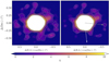 |
Fig. 4. Observed (left panel) and field star cleaned (right panel) stellar density maps adding up all stars in the four MS strips of the cluster of Fig. 2. The black circle centered on the cluster indicates the assumed tidal radius. Contours for η = 1, 2, 4, 6, 8, and 10 are also shown. The different arrows indicate the directions of the proper motion of the cluster (white) and of the Milky Way’s center (gray). |
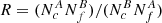
We further analyzed the possibility of tidal deformations across the stellar density map of the cluster, in the sense that preferential orientation toward the Galactic center and along the direction of the orbit of the cluster are expected in the innermost and outermost parts, respectively (Montuori et al. 2007). We followed the recipe applied by Sollima et al. (2011) based on counts of MS strip stars of the cluster in alternate pairs of circular sectors of 90° in width that are located at a given distance from the cluster center and oriented at a position angle (PA) in opposite directions. PA is measured from the north in the anticlockwise direction. We then computed the ratio 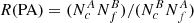 , where A and B are the pair of alternate sectors, and c and f refer to the MS strip of the cluster and a CMD field rectangle defined by 18.5 < g0 (mag) < 22.5 and 1.0 < (g − r)0 (mag) < 1.15. In order to assess the statistical significance of our results, we performed 1000 Monte Carlo realizations using the same number of measured stars distributed randomly in PA and then we obtained the mean and standard deviations of those independent executions. Figure 5 depicts the resulting curves for different annular regions. As suggested by Fig. 4, Fig. 5 shows the existence of a short tidal tail that is nearly aligned with the direction to the Milky Way center, which is in very good agreement with the models of Montuori et al. (2007). The PA’s width of this short tail is also in agreement with S20 (see his Fig. 4). For completeness purposes, we included the directions toward the Milky Way center and of the motion of the cluster in Fig. 4 (right panel).
 |
Fig. 5. Ratio |
We estimated the g surface brightness of the tidal tail observed in Fig. 4, that is, from the stars that were not subtracted by the cleaned, field star CMD procedure, for three different adjacent annulus of 0.1° wide, located between 0.4° and 0.7° from the cluster center. We first calculated the integrated g magnitude (gint) for stars located inside a radius of 0.1° from the cluster center in Fig. 4 (right panel) by summing de DECam g fluxes of individual stars. A normalization constant c was calculated as :

where N0 represents the number of stars used. Then, the integrated magnitudes for the different annular regions were calculated according to:

where N, r1, and r2 represent the number of stars located in an annulus with inner and outer radii r1 and r2, respectively. With the aim of expressing the integrated magnitudes in units of V mag per square arcsec, we used the integrated B − V color for NGC 7099 listed by (= 0.60 mag; Harris 1996, 2010 Edition) and the linear relationship between g and V in terms of the B − V color (Jordi et al. 2006). The resulting surface brightness and its uncertainty computed from the propagation of errors assuming a Poisson statistics turned out to be 31.35 ± 0.11, 31.41 ± 0.11, and 31.44 ± 0.12 mag per square arcsec for the annulus at r = 0.4° −0.5°, 0.5° −0.6°, and 0.6° −0.7°, respectively.
4. Discussion
Recently, S20 presented results of a 5D mixture modeling technique based on Gaia DR2 data of the outer regions of 18 Milky Way globular clusters. He found that NGC 7099 has long tidal tails. Reportedly, those tails are composed by cluster red giant branch (RGB) and MS stars reaching down to ∼1 mag below the MS turnoff of the cluster. This means that S20 used stars that were brighter, on average, than those of our selected MS strip #1 in Fig. 2. At this point, we wonder what caused the different results obtained in the present study compared to those in S20, particularly because MS stars in strips #2 to 4 are expected to be better candidates to trace extra-tidal structures. According to S20 (his Fig. 1), selected MS stars have parallaxes within a range at least 10 times larger than the parallaxes of RGB stars, which means that field stars with loci in the CMD and in the vector point diagram (VPD, proper motion in RA (pmra) vs. proper motion in Dec. (pmdec)) similar to those of the cluster stars could be included in the selected sample. From a comparison of previous studies on the outer regions of Milky Way globular clusters (see Table 1 in Piatti & Carballo-Bello 2020), we also found that results for some globular clusters are distinct from those found in S20. For instance, NGC 1851 and 4590 are known to have long tidal tails, although the were not detected in S20, while NGC 2298, 6341, and 6362 do not seem to have the tails traced in S20. In this respect, we note that it is not straightforward to conclude whether deep photometric-only data sets or shallow proper motion-selected ones are preferable to detect tidal tails. Therefore, it is conceivable that differences can be found in some globular clusters that are subject to different levels of contamination when analyzing them with different data sets.
We used the 5° in radius around NGC 7099 Gaia DR2 (Gaia Collaboration 2016, 2018) database as in S20 to repeat the CMD cleaning procedure applied in Sect. 3 in order to build a stellar density map that is to be compared with the one produced by S20. Figure 6 shows the intrinsic CMD of the inner cluster region used in Fig. 2 that highlights the main features of NGC 7099. Particularly, we chose a strip along the RGB and another one from the MS turnoff down to 2.5 mags underneath. According to Arenou et al. (2018, see Sect. 3), the Gaia DR2 photometry completeness is 90% for stars with G < 19 mag in the inner region of a globular cluster with ∼104 stars/sq deg, so that we deal with basically a complete photometry data set. The adopted fainter limit should likewise be acceptable to guarantee the homogeneity of the completeness. We also used a bandwidth of 0.1° in order to get the highest contrast of tidal tails. We cleaned both strips from field star contamination for a circular area centered on NGC 7099 with a radius equal to 3.53° in order to ensure a reference field star region (3.53° < r < 5°) with an equal cluster area. The Gaia photometry was corrected by reddening using individual E(B − V) values obtained from Schlafly & Finkbeiner (2011), and the relationships AG = 2.44E(B − V) and E(GBP − GRP) = 1.27E(B − V) (Wang & Chen 2019). The observed and cleaned stellar density maps are depicted in Fig. 7. Observed RGB and MS density maps exhibit different spatial distributions, the latter suggesting the existence of tidal tails within a remarkably nonuniform star field spatial distribution. Long tidal tails do not remain in the cleaned, star field density maps, although some hint for short ones are found.
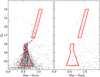 |
Fig. 6. Gaia color–magnitude diagrams of stars in the field of NGC 7099 (r < 0.15°; left panel) and in an annular region of the same area centered on the cluster with an external radius of 0.8° (right panel). The RGB and MS regions used to perform star counts are delineated with red contour lines. |
The above outcomes suggest that stars distributed along the cluster CMD features (e.g., strips in Figs. 2 and 6) located beyond its tidal radius (r > 0.32°) might belong to the Milky Way field. We further used the proper motions of all the stars located within the strips drawn in Fig. 6, which show some particular features. We illustrate them in Fig. 8, where we plotted the VPD for RGB and MS strip stars that are located in three different sky regions, namely, those located inside the tidal radius of the cluster (top panels), those distributed between 0.32° and 3.53° from the cluster center (middle panels), and those adopted as reference field stars (bottom panels). Cluster stars (g0(MS strip) < 19 mag) and RGB strip stars) have a well-defined distribution in the VPD, which we embraced by a red ellipse (top panels). Stars located beyond the cluster radius have a different distribution (middle and bottom panels), with some superposition with that of cluster stars (top panels). For comparison purposes, we superimposed the ellipses in the top panels onto the middle and bottom panels. The middle panel reveals that there are many MS strip stars located outside the cluster with proper motions distinguishable from that of the cluster (most of the stars located outside the ellipses). Particularly, they have g0 mag between 19 and 20.5 mag (see Fig. 6). Most of those stars were eliminated using the CMD cleaning procedure (see Fig. 7).
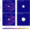 |
Fig. 7. Gaia observed (left panels) and cleaned, field star (right panels) stellar density maps for the cluster RGB and MS strips of Fig. 6. The black circle centered on the cluster indicates the assumed tidal radius. |
From Fig. 8, we conclude that out of all the stars distributed within the RGB and MS strips, some of them have sky projected kinematics similar to that of cluster stars. Therefore, questioning whether those are in fact star cluster members is unavoidable. If we used the CMD cleaning procedure, we would be able to determine that they do not belong to the cluster population, as obtained above. Indeed, from field star contamination, we cleaned the VPD at r < 3.53° from the cluster center, using a star field located between 3.53° and 5° as a reference, similarly as we did for the CMD cleaning. The resulting cleaned, star field stellar density maps for RGB and MS strip stars that share the cluster’s proper motion, whcih were built using the same bandwidth as in Fig. 7, do not show any extra-tidal feature (see Fig. 9, right panels). Finally, we only used the kinematic and parallax information when selecting cluster stars. The top-left panel of Fig. 9 shows the stellar density map built for stars with proper motions within an ellipse centered on (−0.73 mas yr−1, −7.24 mas yr−1), a width = 3.4 mas yr−1, a height = 2.5 mas yr−1, and an angle = 30°, as well as |ϖ| < 5σ(ϖ) (S20), while the bottom-left one depicts the stellar density map after cleaning the cluster field from field contamination, solely based on the kinematic information. As can be seen, there are no remaining signatures of extra-tidal features.
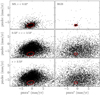 |
Fig. 8. Vector point diagrams for RGB (right panels) and MS (left panels) strips of Fig. 6 for different annular regions. Red ellipses that mostly embrace cluster stars in the top panels were superimposed onto the middle and bottom panels. |
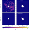 |
Fig. 9. Gaia observed (top-left panel) and cleaned, field star (bottom-left panel) stellar density maps for stars that were only selected from proper motion and parallax criteria. The right panels correspond to RGB and MS stars that remained unsubtracted after the photometric and kinematic cleaning procedures were applied. The black circle centered on the cluster indicates the assumed tidal radius. |
5. Conclusions
In this study, we analyze the outer regions of the Milky Way globular cluster NGC 7099, aiming to identify extra-tidal features. The cluster caught our attention because it was claimed that it might have formed within the accreted Sausage-Enceladus dwarf galaxy and deposited in an inner halo orbit, with a relatively high eccentricity and inclination angle with respect to the Milky Way plane. According to Piatti et al. (2019), globular clusters with orbital parameters similar to those of NGC 7099 have lost relatively more mass by tidal disruption than globular clusters rotating in the Milky Way disk. In the case of NGC 7099, the disrupted mass to the initial mass ratio is 0.30.
We carried out DECam observations that, as far as we are aware, allowed us to build the deepest cluster CMD, reaching ∼6 mags beneath its MS turnoff. Those observed faint MS stars are treated as suitable candidates to trace extra-tidal features, because they are the first to cross the Jacobi radius once they reach the cluster boundary driven by two-body relaxation. Indeed, it has long been observed that the brighter the range of magnitudes considered, the sharper the cluster stellar radial profile.
In order to monitor any differential change in the stellar density map caused by cluster stars with distinct brightnesses, we split the long MS of the cluster into four segments of one mag long each, and we analyzed them separately. We built their respective stellar density maps with a frequently used KDE technique once the magnitudes and colors of the stars were individually corrected by the interstellar extinction. When a statistical decontamination method is used to clean the cluster CMD from field stars, the resulting cleaned stellar density maps show a short tidal tail and some scattered debris. The short tidal tail is nearly oriented to the Milky Way center, as is expected for the innermost parts of tidal tails. We did not find these extra-tidal features when analyzing Gaia data with the same cleaning procedure. In this case, the photometry used is much shallower than the DECam photometry, reaching 2.5 mag below the MS turnoff of the cluster, and the analyzed area is 25 times larger than afforded by our DECam data, so that the reference star field is located much farther from the cluster (3.53° < r < 5.00°).
RGB and MS strip stars that are located inside and outside the cluster tidal radius (0.32°) present distinguishable VPDs, with some superposition. When comparing their VPDs, using the CMD cleaning method separately for stars located within a circle of radius 3.53° with those placed in the reference star field (3.53° < r < 5.00°), we did not find any extra-tidal features. S20 detected long tidal tails; the innermost parts of them were also found from DECam data. Finally, we would like to mention that extra-tidal stars should have distinct velocities that make it possible for them to escape the cluster. Likewise, they are at different Galactocentric distances than the cluster itself, so that they are differently affected by the Milky Way gravitational field (Piatti 2020; Dinnbier & Kroupa 2020).
Acknowledgments
We thank the referee for the thorough reading of the manuscript and timely suggestions to improve it. Support for M.C. is provided by ANID Millennium Science Initiative grant ICN12_009; by Proyecto Basal AFB-170002; and by FONDECYT grant 1171273. Based on observations at Cerro Tololo Inter-American Observatory, NSF’s NOIRLab (Prop. ID 2019B-1003; PI: Carballo-Bello), which is managed by the Association of Universities for Research in Astronomy (AURA) under a cooperative agreement with the National Science Foundation. This project used data obtained with the Dark Energy Camera (DECam), which was constructed by the Dark Energy Survey (DES) collaboration. Funding for the DES Projects has been provided by the US Department of Energy, the US National Science Foundation, the Ministry of Science and Education of Spain, the Science and Technology Facilities Council of the United Kingdom, the Higher Education Funding Council for England, the National Center for Supercomputing Applications at the University of Illinois at Urbana-Champaign, the Kavli Institute for Cosmological Physics at the University of Chicago, Center for Cosmology and Astro-Particle Physics at the Ohio State University, the Mitchell Institute for Fundamental Physics and Astronomy at Texas A&M University, Financiadora de Estudos e Projetos, Fundação Carlos Chagas Filho de Amparo à Pesquisa do Estado do Rio de Janeiro, Conselho Nacional de Desenvolvimento Científico e Tecnológico and the Ministério da Ciência, Tecnologia e Inovação, the Deutsche Forschungsgemeinschaft and the Collaborating Institutions in the Dark Energy Survey. The Collaborating Institutions are Argonne National Laboratory, the University of California at Santa Cruz, the University of Cambridge, Centro de Investigaciones Enérgeticas, Medioambientales y Tecnológicas–Madrid, the University of Chicago, University College London, the DES-Brazil Consortium, the University of Edinburgh, the Eidgenössische Technische Hochschule (ETH) Zürich, Fermi National Accelerator Laboratory, the University of Illinois at Urbana-Champaign, the Institut de Ciències de l’Espai (IEEC/CSIC), the Institut de Física d’Altes Energies, Lawrence Berkeley National Laboratory, the Ludwig-Maximilians Universität München and the associated Excellence Cluster Universe, the University of Michigan, NSF’s NOIRLab, the University of Nottingham, the Ohio State University, the OzDES Membership Consortium, the University of Pennsylvania, the University of Portsmouth, SLAC National Accelerator Laboratory, Stanford University, the University of Sussex, and Texas A&M University.
References
- Arenou, F., Luri, X., Babusiaux, C., et al. 2018, A&A, 616, A17 [Google Scholar]
- Balbinot, E., & Gieles, M. 2018, MNRAS, 474, 2479 [NASA ADS] [CrossRef] [Google Scholar]
- Baumgardt, H., Hilker, M., Sollima, A., & Bellini, A. 2019, MNRAS, 482, 5138 [Google Scholar]
- Bellazzini, M., Ferraro, F. R., & Ibata, R. 2003, AJ, 125, 188 [NASA ADS] [CrossRef] [Google Scholar]
- Belokurov, V., Zucker, D. B., Evans, N. W., et al. 2006, ApJ, 642, L137 [NASA ADS] [CrossRef] [Google Scholar]
- Belokurov, V., Erkal, D., Evans, N. W., Koposov, S. E., & Deason, A. J. 2018, MNRAS, 478, 611 [NASA ADS] [CrossRef] [Google Scholar]
- Carballo-Bello, J. A. 2019, MNRAS, 486, 1667 [NASA ADS] [CrossRef] [Google Scholar]
- Carballo-Bello, J. A., Sollima, A., Martínez-Delgado, D., et al. 2014, MNRAS, 445, 2971 [NASA ADS] [CrossRef] [Google Scholar]
- Carballo-Bello, J. A., Corral-Santana, J. M., Martínez-Delgado, D., et al. 2017, MNRAS, 467, L91 [Google Scholar]
- Carballo-Bello, J. A., Martínez-Delgado, D., Navarrete, C., et al. 2018, MNRAS, 474, 683 [NASA ADS] [CrossRef] [Google Scholar]
- Dinnbier, F., & Kroupa, P. 2020, A&A, 640, A84 [EDP Sciences] [Google Scholar]
- Flaugher, B., Diehl, H. T., Honscheid, K., et al. 2015, AJ, 150, 150 [Google Scholar]
- Forbes, D. A., & Bridges, T. 2010, MNRAS, 404, 1203 [NASA ADS] [Google Scholar]
- Fukugita, M., Ichikawa, T., Gunn, J. E., et al. 1996, AJ, 111, 1748 [NASA ADS] [CrossRef] [Google Scholar]
- Gaia Collaboration (Prusti, T., et al.) 2016, A&A, 595, A1 [NASA ADS] [CrossRef] [EDP Sciences] [Google Scholar]
- Gaia Collaboration (Brown, A. G. A., et al.) 2018, A&A, 616, A1 [NASA ADS] [CrossRef] [EDP Sciences] [Google Scholar]
- Harris, W. E. 1996, AJ, 112, 1487 [NASA ADS] [CrossRef] [Google Scholar]
- Helmi, A., Babusiaux, C., Koppelman, H. H., et al. 2018, Nature, 563, 85 [NASA ADS] [CrossRef] [Google Scholar]
- Ibata, R. A., Gilmore, G., & Irwin, M. J. 1994, Nature, 370, 194 [NASA ADS] [CrossRef] [Google Scholar]
- Ibata, R. A., Malhan, K., Martin, N. F., & Starkenburg, E. 2018, ApJ, 865, 85 [NASA ADS] [CrossRef] [Google Scholar]
- Jordi, K., Grebel, E. K., & Ammon, K. 2006, A&A, 460, 339 [NASA ADS] [CrossRef] [EDP Sciences] [Google Scholar]
- Koposov, S. E., Belokurov, V., Evans, N. W., et al. 2012, ApJ, 750, 80 [NASA ADS] [CrossRef] [Google Scholar]
- Kuzma, P. B., Da Costa, G. S., Mackey, A. D., & Roderick, T. A. 2016, MNRAS, 461, 3639 [NASA ADS] [CrossRef] [Google Scholar]
- Majewski, S. R., Skrutskie, M. F., Weinberg, M. D., & Ostheimer, J. C. 2003, ApJ, 599, 1082 [NASA ADS] [CrossRef] [Google Scholar]
- Massari, D., Koppelman, H. H., & Helmi, A. 2019, A&A, 630, L4 [NASA ADS] [CrossRef] [EDP Sciences] [Google Scholar]
- Mateu, C., Read, J. I., & Kawata, D. 2018, MNRAS, 474, 4112 [NASA ADS] [CrossRef] [Google Scholar]
- Montuori, M., Capuzzo-Dolcetta, R., Di Matteo, P., Lepinette, A., & Miocchi, P. 2007, ApJ, 659, 1212 [NASA ADS] [CrossRef] [Google Scholar]
- Myeong, G. C., Evans, N. W., Belokurov, V., Sanders, J. L., & Koposov, S. E. 2018, ApJ, 863, L28 [NASA ADS] [CrossRef] [Google Scholar]
- Odenkirchen, M., Grebel, E. K., Dehnen, W., et al. 2003, AJ, 126, 2385 [NASA ADS] [CrossRef] [Google Scholar]
- Piatti, A. E. 2017a, ApJ, 846, L10 [NASA ADS] [CrossRef] [Google Scholar]
- Piatti, A. E. 2017b, ApJ, 834, L14 [NASA ADS] [CrossRef] [Google Scholar]
- Piatti, A. E. 2017c, MNRAS, 465, 2748 [NASA ADS] [CrossRef] [Google Scholar]
- Piatti, A. E. 2018, MNRAS, 477, 2164 [NASA ADS] [CrossRef] [Google Scholar]
- Piatti, A. E. 2019, ApJ, 882, 98 [NASA ADS] [CrossRef] [Google Scholar]
- Piatti, A. E. 2020, A&A, 639, A55 [CrossRef] [EDP Sciences] [Google Scholar]
- Piatti, A. E., & Bica, E. 2012, MNRAS, 425, 3085 [NASA ADS] [CrossRef] [Google Scholar]
- Piatti, A. E., & Carballo-Bello, J. A. 2019, MNRAS, 485, 1029 [NASA ADS] [CrossRef] [Google Scholar]
- Piatti, A. E., & Carballo-Bello, J. A. 2020, A&A, 637, L2 [CrossRef] [EDP Sciences] [Google Scholar]
- Piatti, A. E., & Fernández-Trincado, J. G. 2020, A&A, 635, A93 [CrossRef] [EDP Sciences] [Google Scholar]
- Piatti, A. E., Cole, A. A., & Emptage, B. 2018, MNRAS, 473, 105 [NASA ADS] [CrossRef] [Google Scholar]
- Piatti, A. E., Webb, J. J., & Carlberg, R. G. 2019, MNRAS, 489, 4367 [NASA ADS] [CrossRef] [Google Scholar]
- Schlafly, E. F., & Finkbeiner, D. P. 2011, ApJ, 737, 103 [NASA ADS] [CrossRef] [Google Scholar]
- Sollima, A. 2020, MNRAS, 495, 2222 [CrossRef] [Google Scholar]
- Sollima, A., Martínez-Delgado, D., Valls-Gabaud, D., & Peñarrubia, J. 2011, ApJ, 726, 47 [NASA ADS] [CrossRef] [Google Scholar]
- Stetson, P. B. 1987, PASP, 99, 191 [Google Scholar]
- Valdes, F., Gruendl, R., & DES Project 2014, in Astronomical Data Analysis Software and Systems XXIII, eds. N. Manset, & P. Forshay, ASP Conf. Ser., 485, 379 [NASA ADS] [Google Scholar]
- Vanderbeke, J., De Propris, R., De Rijcke, S., et al. 2015, MNRAS, 450, 2692 [NASA ADS] [CrossRef] [Google Scholar]
- VanderPlas, J., Connolly, A. J., Ivezic, Z., & Gray, A. 2012, Proceedings of Conference on Intelligent Data Understanding (CIDU), 47 [Google Scholar]
- Wang, S., & Chen, X. 2019, ApJ, 877, 116 [NASA ADS] [CrossRef] [Google Scholar]
All Figures
|
Fig. 1. Reddening map across the field of NGC 7099. The red and black circles are of 0.32° and 0.73° in radius, respectively. The black circle separates two areas of the same size. |
| In the text | |
|
Fig. 2. CMDs of stars in the field of NGC 7099 (r < 0.15°; left panel) and in an annular region of the same area centered on the cluster with an external radius of 0.8° (right panel). The four regions along the MS of the cluster that were used to perform star counts are delineated with red contour lines. |
| In the text | |
|
Fig. 3. Observed (left panels) and field star cleaned (right panels) stellar density maps for the four MS strips of the cluster of Fig. 2 as labeled at the top-left margin of each panel. The black circle centered on the cluster indicates the assumed tidal radius. Contours for η = 1, 2, 4, 6, 8, and 10 are also shown; the colors follow the coding shown at the bottom of each panel. |
| In the text | |
|
Fig. 4. Observed (left panel) and field star cleaned (right panel) stellar density maps adding up all stars in the four MS strips of the cluster of Fig. 2. The black circle centered on the cluster indicates the assumed tidal radius. Contours for η = 1, 2, 4, 6, 8, and 10 are also shown. The different arrows indicate the directions of the proper motion of the cluster (white) and of the Milky Way’s center (gray). |
| In the text | |
|
Fig. 5. Ratio |
| In the text | |
|
Fig. 6. Gaia color–magnitude diagrams of stars in the field of NGC 7099 (r < 0.15°; left panel) and in an annular region of the same area centered on the cluster with an external radius of 0.8° (right panel). The RGB and MS regions used to perform star counts are delineated with red contour lines. |
| In the text | |
|
Fig. 7. Gaia observed (left panels) and cleaned, field star (right panels) stellar density maps for the cluster RGB and MS strips of Fig. 6. The black circle centered on the cluster indicates the assumed tidal radius. |
| In the text | |
|
Fig. 8. Vector point diagrams for RGB (right panels) and MS (left panels) strips of Fig. 6 for different annular regions. Red ellipses that mostly embrace cluster stars in the top panels were superimposed onto the middle and bottom panels. |
| In the text | |
|
Fig. 9. Gaia observed (top-left panel) and cleaned, field star (bottom-left panel) stellar density maps for stars that were only selected from proper motion and parallax criteria. The right panels correspond to RGB and MS stars that remained unsubtracted after the photometric and kinematic cleaning procedures were applied. The black circle centered on the cluster indicates the assumed tidal radius. |
| In the text | |
Current usage metrics show cumulative count of Article Views (full-text article views including HTML views, PDF and ePub downloads, according to the available data) and Abstracts Views on Vision4Press platform.
Data correspond to usage on the plateform after 2015. The current usage metrics is available 48-96 hours after online publication and is updated daily on week days.
Initial download of the metrics may take a while.