| Issue |
A&A
Volume 683, March 2024
|
|
|---|---|---|
| Article Number | A151 | |
| Number of page(s) | 7 | |
| Section | Galactic structure, stellar clusters and populations | |
| DOI | https://doi.org/10.1051/0004-6361/202348534 | |
| Published online | 15 March 2024 | |
First deep search of tidal tails in the Milky Way globular cluster NGC 6362
1
Instituto Interdisciplinario de Ciencias Básicas (ICB), CONICET-UNCUYO, Padre J. Contreras 1300, M5502JMA Mendoza, Argentina
e-mail: This email address is being protected from spambots. You need JavaScript enabled to view it.
2
Consejo Nacional de Investigaciones Científicas y Técnicas (CONICET), Godoy Cruz 2290, C1425FQB Buenos Aires, Argentina
Received:
9
November
2023
Accepted:
16
January
2024
Abstract
I present results of the analysis of a set of images obtained in the field of the Milky Way globular cluster NGC 6362 using the Dark Energy Camera, which is mounted in the 4.0 m Victor Blanco telescope of the Cerro-Tololo Interamerican Observatory. The cluster was selected as a science case for deep high-quality photometry because of the controversial observational findings and theoretical predictions on the existence of cluster tidal tails. The collected data allowed me to build an unprecedented deep cluster field color-magnitude diagram, from which I filtered stars to produce a stellar density map, to trace the stellar density variation as a function of the position angle for different concentric annuli centered on the cluster, and to construct a cluster stellar density radial profile. I also built a stellar density map from a synthetic color-magnitude diagram generated from a model of the stellar population distribution in the Milky Way. The entire analysis approach converged toward a relatively smooth stellar density between 1 and ∼3.8 cluster Jacobi radii, with a slight difference smaller than two times the background stellar density fluctuation between the mean stellar density of the southeastern hemisphere and that of the northwestern one, with the latter being higher. Moreover, the spatial distribution of the recently claimed tidal tail stars agrees well not only with the observed composite star field distribution, but also with the region least affected by interstellar absorption. Nevertheless, I detected a low stellar density excess around the cluster’s Jacobi radius, from which I conclude that NGC 6362 presents a thin extra tidal halo.
Key words: methods: observational / techniques: polarimetric / globular clusters: general / globular clusters: individual: NGC 6362
© The Authors 2024
 Open Access article, published by EDP Sciences, under the terms of the Creative Commons Attribution License (https://creativecommons.org/licenses/by/4.0), which permits unrestricted use, distribution, and reproduction in any medium, provided the original work is properly cited.
This article is published in open access under the Subscribe to Open model. This email address is being protected from spambots. You need JavaScript enabled to view it. to support open access publication.
1. Introduction
The recent stringent compilation of Milky Way globular clusters with robust detections of extra-tidal structures includes only one bulge-disk globular cluster with tidal tails (NGC 6362, Zhang et al. 2022), while Carlberg & Grillmair (2021) did not include any bulge globular cluster in their search for dark matter in the globular clusters’ outskirts. This brief overview illustrates that bulge globular clusters have not generally been targeted for studies of their outermost stellar structures, which are fundamental for our understanding of whether they formed in dark matter minihaloes (Starkman et al. 2020; Baumgardt & Vasiliev 2021; Wan et al. 2021); their association with destroyed dwarf progenitors (Carballo-Bello et al. 2014; Mackey et al. 2019); their dynamical history as a consequence of the interaction with the Milky Way (Hozumi & Burkert 2015; de Boer et al. 2019; Piatti & Carballo-Bello 2020); among others. Therefore, there are strong motivations to detect and characterize tidal tails in bulge globular clusters, making it a compelling field of research.
Zhang et al. (2022) classified NGC 6362 as a globular cluster with tidal tails based on the work by Kundu et al. (2019), who found 259 of them spread over an area of ∼4.1 deg2 centered on the cluster. These stars should be placed beyond the cluster’s Jacobi radius (rJ), which defines the surface from which cluster stars are no longer bound to the cluster and are lost in the form of tidal tails. The value of rJ depends on the Milky Way potential at the position of the globular cluster and its orbit around the Milky Way. For NGC 6362, Piatti et al. (2019) derived rJ = 0.26 deg. Kundu et al. (2019) also showed that the cluster is moving in a chaotic orbit. However, Mestre et al. (2020) compared the behavior of simulated streams embedded in chaotic and non-chaotic regions of the phase space and found that typical gravitational potentials of host galaxies can sustain chaotic orbits, which in turn do reduce the time interval during which streams can be detected. This explains why tidal tails in some globular clusters are washed out after they are generated to the point at which it is impossible to detect them. NGC 5139, with an apogalactocentric distance of 7.0 kpc, is indeed the innermost globular cluster with observed tidal tails; NGC 6362 is at 5.5 kpc from the Galactic center (Baumgardt & Vasiliev 2021).
Given that the structures I am interested in –the tidal tails of NGC 6362– are mainly composed of low-mass main sequence stars, it is necessary to map the faint end of the cluster color-magnitude diagram (CMD), allowing me to determine the outer structure of the cluster with excellent statistics and to truly map the outskirts to look for tidal tails. It is widely accepted that Milky Way globular clusters have lost most of their masses through three main processes, namely: stellar evolution, two-body relaxation, and tidal heating caused by the Milky Way’s gravitational field (Piatti et al. 2019, and reference therein). Studies on the external regions of Milky Way globular clusters use such faint main sequence stars to detect tidal tails because they are more numerous (Carballo-Bello et al. 2012). I note that the Gaia data used by Kundu et al. (2019) to select tidal tail stars barely reach the cluster’s main sequence turnoff (G0 ∼ 19 mag).
In Sect. 2 I describe the deep wide-field observations carried out to investigate the existence of tidal tails in the outskirts of NGC 6362. The analysis of the obtained CMD and stellar density maps is described in Sect. 3, while Sect. 4 deals with the discussion of the distribution of stars and gas in the Milky Way along the cluster’s line of sight. In Sect. 5 I summarize the main conclusions of this work.
2. Observational data
I employed the Dark Energy Camera (DECam, Flaugher et al. 2015), an array of 62 identical chips with a scale of 0.263 arcsec pixel−1 that provides a 3 deg2 field of view, attached to the prime focus of the 4-m Blanco telescope at the Cerro Tololo Inter-American Observatory (CTIO). The collected data are part of the observing program 2023A-627924 (PI: A. Piatti) and consist of 4 × 400 s g and 1 × 100 s + 7 × 400 s i exposures, respectively. The images’ quality is better than 0.9 arcsec. The DECam community pipeline team processed the images by applying the highest performance instrumental calibrations, eliminating one CCD of problematic usefulness. The CCD images were trimmed of bad edge pixels, and reference bias and dome flat files were created for each night in order to remove the instrumental signature from the science data. The images were then resampled to a standard orientation and pixel scale at a standard tangent point. Finally, the DECam community pipeline applied photometric calibrations.
I split the entire DECam field of view into nine equal squared areas of ∼0.67 deg per side, and for each of these subfields I performed point spread function (PSF) photometry using the DAOPHOT/ALLSTAR suite of programs (Stetson et al. 1990). For each subfield, I obtained a quadratically varying PSF by fitting ∼2200 stars deg2 once I eliminated the neighbors using a preliminary PSF derived from the brightest, least contaminated 900 stars deg2. Both groups of PSF stars were interactively selected. I then used the ALLSTAR program to apply the resulting PSF to the identified stellar objects and to create a subtracted image, which was used to find and measure magnitudes of additional fainter stars. This procedure was repeated three times for each subfield. In order to properly match a g subfield with the corresponding i one, I used the IRAF.IMMATCH@WCSMAP task, and then stand-alone DAOMATCH/DAOMASTER routines1 to gather pixel coordinates, g and i magnitudes with their respective errors, sharpness, and χ values for all the measured sources. Finally, I assigned RA and Dec coordinates to each stars using the WCSTOOL package2 and kept sources with |sharpness| < 0.5 in order to remove bad pixels, unresolved double stars, cosmic rays, and background galaxies from the photometric catalog.
3. Data analysis
The region onto which NGC 6362 is projected is affected by interstellar extinction that varies with the position in the sky. In order to reproduce the interstellar extinction map toward the cluster, I retrieved the E(B − V) values as a function of RA and Dec from Schlafly & Finkbeiner (2011), provided by the NASA/IPAC Infrared Science Archive3 for the entire analyzed area. Figure 1 illustrates the resulting extinction map, which reveals that along the cluster’s line of sight the interstellar absorption is relatively low, with a maximum difference between the most and least reddened regions of ΔE(B − V)≲0.05 mag. Based on Fig. 1, I assigned individual E(B − V) values to the measured stars according to their positions in the sky. In order to correct the observed magnitudes and colors by interstellar extinction, I used the individual E(B − V) values and the Aλ/AV coefficients given by Wang & Chen (2019). Figure 2 shows the wealth of information that I produced from the observed images, where a nearly 3 mag long well-defined cluster’s main sequence is clearly visible, alongside with the cluster’s main sequence turnoff, subgiant, and the fainter segment of the giant branches. In order to highlight the cluster’s CMD features, I used all the measured stars located within a circle of radius equal to two times the cluster’s half-mass radius (rh = 0.11 deg, Baumgardt & Vasiliev 2021). The positions of stars located inside 2 × rh are satisfactorily reproduced by an isochrone (Bressan et al. 2012) for the cluster’s age (12 Gyr) and metallicity ([Fe/H] = −1.07 dex) (Gontcharov et al. 2023). Figure 2 also shows that the photometric uncertainties of magnitude and color for the faintest observed cluster’s stars are smaller than ∼0.05 mag. NGC 6362 appears projected onto a crowded star field (gray dots in Fig. 2).
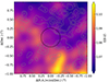 |
Fig. 1. Interstellar extinction (E(B − V)) map across the observed NGC 6362 field. The black circle represents the cluster’s Jacobi radius (0.26 deg), while the gray contours correspond to isodensity levels of the tidal tail stars selected by Kundu et al. (2019). |
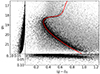 |
Fig. 2. CMD for all the measured stars in the field of NGC 6362, with their respective photometric errors. Black and gray dots represent stars located inside and outside a circle of radius equals to two times the cluster’s half-mass radius (0.11 deg), respectively. The red line is an isochrone for the cluster’s age (12 Gyr) and metallicity ([Fe/H] = −1.07 dex) (Gontcharov et al. 2023). |
The strategy chosen to uncover the spatial distribution of stars that formed within NGC 6362 and are now observed beyond its Jacobi radius consists in statistically identifying cluster’s main sequence stars located outside that radius, following the recipe outlined by Zhang et al. (2022). For that purpose, I first defined a region along the cluster’s main sequence, from g0 = 18 mag down to g0 = 21.5 mag and, second, I built a stellar density map for all the stars that fall within that CMD region. Unfortunately, this approach is not able to discern the cluster membership of these stars. For such an assessment, I need additional information, such as proper motions, radial velocities, and metallicities. As far as I am aware, because of the relative faintness of the involved stars, this information in still unavailable. Nevertheless, field stars within the cluster’s main sequence region are expected to be distributed throughout the entire field, so that cluster stars arise as particular shaped stellar overdensities forming an extended envelope, extra-tidal debris, or tidal tails (Piatti & Carballo-Bello 2020).
The cluster’s main sequence region was devised from the following two steps. I first traced the cluster’s main sequence ridge line, and then I fixed the color width of the devised region as a function of the magnitude. Both steps were carried out using the stars located within 2 × rh from the cluster center, that is, those black points in Fig. 2. The cluster’s main sequence ridge line was determined by computing the median of the color distribution for magnitude intervals of Δg0 = 0.1 mag, while their widths correspond to the derived color standard deviations. Figure 3 depicts a Hess diagram for the employed stars and the various generated curves, namely: the cluster’s main sequence ridge line (red), the lower and upper limits of the cluster’s main sequence colors (orange), and the cluster’s main sequence limits (magenta) corresponding to the mode of the color error distribution (see, also, the trend of errors in Fig. 2). As can be seen, the photometric errors are notably smaller than the adopted intrinsic width of the cluster’s main sequence.
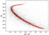 |
Fig. 3. Hess diagram for the stars located within 2 × rh from the cluster center. The traced cluster’s main sequence ridge line (red), its defined lower and upper color limits (orange), and those corresponding to the mode of the color error distribution (magenta) are superimposed, respectively. |
I made use of the scikit-learn software machine learning library (Pedregosa et al. 2011) and its Gaussian kernel density estimator (KDE) to build the stellar density map for the observed field around NGC 6362, using all the stars distributed within the cluster’s main sequence region. I employed a grid of 500 × 500 boxes onto the DECam field and used a range of values for the bandwidth from 0.01° up to 0.1° in steps of 0.01° in order to apply the KDE to each generated box. I adopted a bandwidth of 0.05° as the optimal value, as guided by scikit-learn. Figure 4 shows the resulting density map, where I used a maximum level of 2 stars arcmin−2 in order to highlight lower density levels. The observed spatial pattern of stars located in the cluster’s main sequence region shows a nearly rounded distribution inside the Jacobi radius and no obvious trail of tidal tails outside it, but a nearly smooth stellar distribution over the entire observed field, as expected for a composite star field population. With the aim of quantifying such a trend, I used three different concentric annuli around the cluster center and measured the stellar densities in angular sectors of 10 deg wide. The upper panel of Fig. 5 illustrates the behavior of the stellar density as a function of the position angle, measured from north to east. As can be seen, the three stellar density profiles around the cluster are similar, with fluctuations that mostly vary around a mean value of 0.48 stars arcmin−2 in an amount of σ = 0.11 stars arcmin−2. I then computed the deviation from the mean value in the field in units of the standard deviation, that is, η = (signal − mean value)/standard deviation. From the bottom panel of Fig. 5, I infer that there are some regions, located particularly in the outer northwestern hemisphere, with η ≳ 2, which implies a significance level larger than 95%.
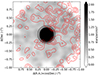 |
Fig. 4. Stellar density map of stars distributed within the cluster’s main sequence region. The black circle represents the cluster’s Jacobi radius, while the red contours correspond to the stellar density levels of the stars selected by Kundu et al. (2019) (see Fig. 6). |
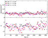 |
Fig. 5. Stellar density as a function of the position angle for three different concentric annuli centered on NGC 6362, as indicated in the top panel. The solid and dotted lines represent the mean and standard deviation of all the plotted points. The significance (η) of the stellar density over the mean background value is depicted in the bottom panel. |
4. Analysis and discussion
Kundu et al. (2019) selected cluster stars (g0 ≲ 18.0 mag) located beyond the cluster’s Jacobi radius based on astrometry-filtering criteria. They appear in the CMD distributed along the cluster subgiant and red giant branches, in addition to the horizontal branch. Particularly, Kundu et al. (2019) restricted cluster stars to have proper motions within 3σ from the mean cluster proper motion. This criterion, which is helpful for identifying cluster stars within the cluster body, could fail when applied to stars that formed in the cluster that later abandoned it. This is because of tidal tail stars have sped up their pace in order to escape the cluster. There are, additionally, other reasons that can contribute to make the proper motion of tidal tail stars different from the mean cluster proper motion, among them are the projection effects of the tidal tails, the Milky Way tidal interaction, and the intrinsic kinematic agitation of a stellar stream (Wan et al. 2023). Likewise, it is possible to find field stars projected along the cluster line of sight that share proper motions similar to cluster stars (Piatti et al. 2023).
I used the Gaia DR2 data (Gaia Collaboration 2016, 2018) from Kundu et al. (2019) for their selected 259 extra-tidal stars to build a stellar density map following the same precepts described above to construct Fig. 4. Figure 6 shows the resulting stellar density map, to which I also traced different contour levels. The stars seem to be preferentially distributed across the northwestern hemisphere, where I also unveiled a slight excess with respect to the southeastern hemisphere (Δη ∼ 2) for stars located along the cluster’s main sequence region (g0 > 18.0 mag). This means that, independently of the chosen magnitude range along the cluster CMD, stars are distributed across the observed DECam field following a similar spatial pattern. I also note that Fig. 2 reveals a large population of field stars (gray dots) superimposed onto the cluster CMD features. As for comparison purposes, I overplotted the contour levels of the stars of Kundu et al. (2019) onto the stellar density map of the cluster’s main sequence stars (see Fig. 4), and onto the reddening map (see Fig. 1). Their spatial distribution could suggest that they are confined within the lower reddening regions. Nevertheless, the variation in the reddening across the field is not so high (ΔE(B − V)≲0.05 mag) as to expect a variation in the stellar density of these relatively bright stars due to interstellar absorption.
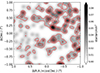 |
Fig. 6. Stellar density map for the tidal tail stars selected by Kundu et al. (2019), with contour levels corresponding to 0.02, 0.035, and 0.05 stars arcmin2. |
I addressed the issue of whether the spatial distribution of the stars selected by Kundu et al. (2019) really represent extra-tidal features of NGC 6362. If they were confirmed, then the slightly stellar excess found from stars distributed within the cluster’s main sequence region could also be evidence of the presence of such extra-tidal structures. Furthermore, they would be very low stellar density tidal tails that do not surpass η = 3. According to Piatti & Carballo-Bello (2020), Milky Way globular clusters can exhibit tidal tails and extended envelopes or they do not show any extra-tidal structures. Examining the shapes of extra-tidal structures of nearly 50 studied globular clusters (Zhang et al. 2022, and references therein) has led me to conclude that extended envelope stellar distributions are functions of the distance to the cluster center, and no angular direction arises as preferential. In turn, tidal tails are well-collimated stellar structures that emerge from the cluster body in two directions, namely, the leading and the trailing tails, respectively. Unfortunately, neither an extended envelope nor tidal tails can be recognized from the spatial distribution of stars selected by Kundu et al. (2019) and in this work (see Fig. 4).
The presence of tidal tails in some globular clusters and the absence of them in others is still a topic of debate. Piatti & Carballo-Bello (2020) explored different kinematical and structural parameter spaces, and found that globular clusters behave similarly, irrespective of the presence of extended envelopes or tidal tails, or the absence thereof. Zhang et al. (2022) showed that globular clusters with tidal tails or extended envelopes have apogalactocentric distances ≳5 kpc, a behavior previously noticed by Piatti (2021), who suggested that the lack of detection of tidal tails in bulge globular clusters could be due to the reduced diffusion time of tidal tails by the kinematically chaotic nature of the orbits of these globular clusters (Kundu et al. 2019), thus shortening the time interval during which the tidal tails can be detected. Recently, Weatherford et al. (2023) reexamined the behavior of potential escapers in globular clusters dynamically evolving along chaotic orbits and found diffusion times shorter than 100 Myr. NGC 6362 is a dynamically evolving globular cluster with a significant internal rotation (Dalessandro et al. 2021).
I investigated the possibility that the spatial distribution of the selected stars of Kundu et al. (2019) (see Fig. 6) can be due to the expected stellar density of Milky Way field stars along the cluster’s line of sight. For that purpose, I made used of TRILEGAL4 (Girardi et al. 2005), a stellar population synthesis code that allows changes in the star formation rate, age-metallicity relation, initial mass function, geometry of Milky Way components, among others. I used 81 adjacent squared regions of 0.0625 deg2 each, which cover the entire observed DECam field uniformly. I generated individual CMDs for each subfield and then counted the number of stars located within the cluster’s main sequence region, similarly to what I did to build Fig. 4.
I chose the DECam photometric system, a limiting magnitude of g, i = 23 mag, and a distance modulus resolution of the Milky Way components of 0.1 mag. I set the initial mass function according to Kroupa (2002), a binary fraction of 0.3 with a mass ratio larger than 0.7. The interstellar extinction was modeled by an exponential disk with a scale height hz = 100 pc, a scale length hR = 3200 pc, and a visual absorption variation ∂AV/∂R = 0.00015 mag pc−1 (Li et al. 2018), with the Sun position at R⊙ = 8300 pc and z⊙ = 15 pc (Monteiro et al. 2021). The Milky Way halo, thin and thick disks, and bulge were modeled as follows: the halo was represented by an oblate r1/4 spheroid with an effective radius rh = 2698.93 pc, an oblateness qh = 0.583063, and Ω = 0.0001 M⊙ pc−3. The halo star formation rate and age-metallicity relationship are those given by Ryan & Norris (1991). The thin disk is described by an exponential disk along z and R with a scale height increasing with age: hz = 94.690 × (1 + age/5.55079 × 109)1.6666, the scale length hR = 2913.36 pc, and there is an outer cutoff at 15 000 pc. I used a two-step star formation rate, the age-metallicity relationship with α enrichment given by Fuhrmann (1998), and Σ = 55.4082 M⊙ pc−2. The thick disk is also represented by an exponential disk in both z and R directions, with scale height hz = .800 pc, scale length hR = 2394.07 pc, and an outer cutoff at 15 000 pc; Ω = 0.001 M⊙ pc−3. I adopted a constant star formation rate and Z = 0.008 with σ[M/H] = 0.1 dex. Finally, I assumed a triaxial bulge with a scale length of 2500 pc and a truncation scale length of 95 pc, in addition to y/x and z/x axial ratios of 0.68 and 0.31, respectively. The angle between the direction along the bar and that from the Sun to the Milky Way center was set in 15 deg, and Ω = 406 M⊙ pc−3. Its star formation rate and age-metallicity relationship were taken from Zoccali et al. (2003).
Figure 7 illustrates the resulting synthetic CMD for the entire studied field, which compares well with that obtained from the observed DECam field (see Fig. 2), while Fig. 8 depicts the stellar density map built from TRILEGAL stars distributed within the cluster’s main sequence region. At a first glance, there is a similarity between the synthetic stellar density map and the spatial distribution of the stars selected by Kundu et al. (2019), which poses the possibility that they could belong to the composite star field population rather than being NGC 6362 tidal tail stars.
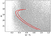 |
Fig. 7. Synthetic CMD generated using TRILEGAL for the studied Milky Way region (see text for details). The red lines represent the devised cluster’s main sequence region. |
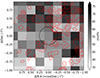 |
Fig. 8. Stellar density map built from star counts of stars distributed within the cluster’s main sequence region generated using TRILEGAL (see text for details). The red contour levels represent the spatial distribution of stars selected by Kundu et al. (2019). The black circle represents the cluster’s Jacobi radius. |
I finally built the cluster stellar density radial profile using the stars distributed within the main sequence region. I counted the number of stars distributed inside boxes of 0.01 deg up to 0.05 deg per side, increasing by steps of 0.01 deg a side, and then built the corresponding radial profiles. This procedure allowed me to extend the radial profile far from the cluster center, where the area of the observed DECam field does not entirely cover those of concentric annuli centered on the cluster. The resulting average radial profile is depicted with open circles in Fig. 9. As expected, the background level is clearly visible across an extended region. I then subtracted from the observed radial profile the mean value of the background stellar density derived above and superimposed to that background-corrected radial profile (filled circles) a King (1962) profile with the core and tidal radius taken from Baumgardt & Hilker (2018). As can be seen, the profile of King (1962) matches the cluster’s radial profile very well, which exhibits an excess of stars following a power law distribution with a slope of 4.0. The latter is remarkably different from the values obtained for Milky Way globular clusters with extended envelopes (slope ∼1; e.g., Olszewski et al. 2009; Piatti 2017). Although the deviation of the radial profile from the profile of is visible, I argue that it does not reveal an extended envelope, but a thin nonuniform low stellar density halo. This outcome is in very good agreement with the slight difference found between the northwestern and southeastern outer hemispheres from the stellar density map.
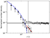 |
Fig. 9. Observed and background-corrected normalized stellar density profiles represented by open and filled circles, respectively. Error bars are also shown. The blue curve represents the King’s model for the core and tidal radius of the cluster (Baumgardt & Hilker 2018), while the red line corresponds to a power law with a slope equal to 4.0. Black horizontal and gray vertical lines represent the mean background level and the cluster’s Jacobi radius, respectively. |
5. Conclusions
The study of the outermost regions of Milky Way globular clusters is interesting on its own since it provides clues about a variety of astrophysical topics for which our understanding is far from complete (see Sect. 1). According to a recent study, NGC 6362 presents tidal tails out to ∼2 deg from its center (Kundu et al. 2019), which challenges theoretical predictions for globular clusters in chaotic orbit regimes and orbiting close to the Milky Way bulge. I recognized here a science case and embarked on the first deep search for extra tidal stars throughout an extended region around the cluster.
The collected data consist of images obtained with the 4.0m Blanco telescope (CTIO) that reach nearly 3 mag below the cluster’s main sequence turnoff across an area of ∼3 deg2, a limiting magnitude not achieved by any ground-based observation except for HST data (Dalessandro et al. 2014) for the innermost cluster region. I scrutinized the produced DECam field CMD, from which I selected stars distributed across the entire field and encompassed within the devised cluster’s main sequence region. Using those stars, I built a stellar density map, an azimuthal stellar distribution for different concentric annuli centered on the cluster, and a cluster stellar density radial profile. From the stellar density map, I detected an overall relatively smooth stellar density distribution from the cluster’s Jacobi radius out to nearly 3.8 × rJ, with a slight difference smaller than two times the background stellar density fluctuation between the mean stellar density of the southeastern hemisphere and that of the northwestern one, with the latter being higher. The same trend is observed in the plane of the stellar density as a function of the position angle, and from the stellar radial profile. I finally constructed a stellar density map from a synthetic CMD generated from a model of the stellar population distribution in the Milky Way, which also confirms the above findings.
On the other hand, I produced a stellar density map of the tidal tail stars selected by Kundu et al. (2019) and superimposed the corresponding contour levels over the present stellar density map and that obtained from the synthetic CMD. The tidal tail stars of Kundu et al. (2019) are mainly distributed throughout the northwestern hemisphere, which suggests that they likely belong to the composite star field population. I also examined their spatial distribution with that of the interstellar absorption toward the cluster, and found that they are projected onto the least reddened regions. Nevertheless, I detected a low stellar density excess around the cluster’s Jacobi radius, from which I conclude that NGC 6362 presents a thin extra tidal halo. This outcome is two-fold in very good agreement with the expected relative high cluster star mass lost by disruption (Piatti et al. 2019) and the short diffuse time of tidal tails applicable to this globular cluster.
Programs kindly provided by P.B. Stetson.
Acknowledgments
I thank the referee for the thorough reading of the manuscript and timely suggestions to improve it. This project used data obtained with the Dark Energy Camera (DECam), which was constructed by the Dark Energy Survey (DES) collaboration. Funding for the DES Projects has been provided by the US Department of Energy, the US National Science Foundation, the Ministry of Science and Education of Spain, the Science and Technology Facilities Council of the United Kingdom, the Higher Education Funding Council for England, the National Center for Supercomputing Applications at the University of Illinois at Urbana-Champaign, the Kavli Institute for Cosmological Physics at the University of Chicago, Center for Cosmology and Astro-Particle Physics at the Ohio State University, the Mitchell Institute for Fundamental Physics and Astronomy at Texas A&M University, Financiadora de Estudos e Projetos, Fundação Carlos Chagas Filho de Amparo Pesquisa do Estado do Rio de Janeiro, Conselho Nacional de Desenvolvimento Científico e Tecnológico and the Ministério da Ciência, Tecnologia e Inovação, the Deutsche Forschungsgemeinschaft and the Collaborating Institutions in the Dark Energy Survey. The Collaborating Institutions are Argonne National Laboratory, the University of California at Santa Cruz, the University of Cambridge, Centro de Investigaciones Enérgeticas, Medioambientales y Tecnológicas–Madrid, the University of Chicago, University College London, the DES-Brazil Consortium, the University of Edinburgh, the Eidgenössische Technische Hochschule (ETH) Zürich, Fermi National Accelerator Laboratory, the University of Illinois at Urbana-Champaign, the Institut de Ciències de l’Espai (IEEC/CSIC), the Institut de Física d’Altes Energies, Lawrence Berkeley National Laboratory, the Ludwig-Maximilians Universität München and the associated Excellence Cluster Universe, the University of Michigan, NSF’s NOIRLab, the University of Nottingham, the Ohio State University, the OzDES Membership Consortium, the University of Pennsylvania, the University of Portsmouth, SLAC National Accelerator Laboratory, Stanford University, the University of Sussex, and Texas A&M University. Based on observations at Cerro Tololo Inter-American Observatory, NSF’s NOIRLab (NOIRLab Prop. ID 2023A-627924; PI: A. Piatti), which is managed by the Association of Universities for Research in Astronomy (AURA) under a cooperative agreement with the National Science Foundation. Data for reproducing the figures and analysis in this work will be available upon request to the author.
References
- Baumgardt, H., & Hilker, M. 2018, MNRAS, 478, 1520 [Google Scholar]
- Baumgardt, H., & Vasiliev, E. 2021, MNRAS, 505, 5957 [NASA ADS] [CrossRef] [Google Scholar]
- Bressan, A., Marigo, P., Girardi, L., et al. 2012, MNRAS, 427, 127 [NASA ADS] [CrossRef] [Google Scholar]
- Carballo-Bello, J. A., Gieles, M., Sollima, A., et al. 2012, MNRAS, 419, 14 [Google Scholar]
- Carballo-Bello, J. A., Sollima, A., Martínez-Delgado, D., et al. 2014, MNRAS, 445, 2971 [Google Scholar]
- Carlberg, R. G., & Grillmair, C. J. 2021, ApJ, 922, 104 [NASA ADS] [CrossRef] [Google Scholar]
- Dalessandro, E., Massari, D., Bellazzini, M., et al. 2014, ApJ, 791, L4 [NASA ADS] [CrossRef] [Google Scholar]
- Dalessandro, E., Raso, S., Kamann, S., et al. 2021, MNRAS, 506, 813 [CrossRef] [Google Scholar]
- de Boer, T. J. L., Gieles, M., Balbinot, E., et al. 2019, MNRAS, 485, 4906 [Google Scholar]
- Flaugher, B., Diehl, H. T., Honscheid, K., et al. 2015, AJ, 150, 150 [Google Scholar]
- Fuhrmann, K. 1998, A&A, 338, 161 [NASA ADS] [Google Scholar]
- Gaia Collaboration (Prusti, T., et al.) 2016, A&A, 595, A1 [NASA ADS] [CrossRef] [EDP Sciences] [Google Scholar]
- Gaia Collaboration (Brown, A. G. A., et al.) 2018, A&A, 616, A1 [NASA ADS] [CrossRef] [EDP Sciences] [Google Scholar]
- Girardi, L., Groenewegen, M. A. T., Hatziminaoglou, E., & da Costa, L. 2005, A&A, 436, 895 [NASA ADS] [CrossRef] [EDP Sciences] [Google Scholar]
- Gontcharov, G. A., Khovritchev, M. Y., Mosenkov, A. V., et al. 2023, MNRAS, 518, 3036 [Google Scholar]
- Hozumi, S., & Burkert, A. 2015, MNRAS, 446, 3100 [NASA ADS] [CrossRef] [Google Scholar]
- King, I. 1962, AJ, 67, 471 [Google Scholar]
- Kroupa, P. 2002, Science, 295, 82 [Google Scholar]
- Kundu, R., Fernández-Trincado, J. G., Minniti, D., et al. 2019, MNRAS, 489, 4565 [Google Scholar]
- Li, L., Shen, S., Hou, J., et al. 2018, ApJ, 858, 75 [NASA ADS] [CrossRef] [Google Scholar]
- Mackey, A. D., Ferguson, A. M. N., Huxor, A. P., et al. 2019, MNRAS, 484, 1756 [NASA ADS] [CrossRef] [Google Scholar]
- Mestre, M., Llinares, C., & Carpintero, D. D. 2020, MNRAS, 492, 4398 [NASA ADS] [CrossRef] [Google Scholar]
- Monteiro, H., Barros, D. A., Dias, W. S., & Lépine, J. R. D. 2021, Front. Astron. Space Sci., 8, 62 [NASA ADS] [CrossRef] [Google Scholar]
- Olszewski, E. W., Saha, A., Knezek, P., et al. 2009, AJ, 138, 1570 [NASA ADS] [CrossRef] [Google Scholar]
- Pedregosa, F., Varoquaux, G., Gramfort, A., et al. 2011, J. Mach. Learn. Res., 12, 2825 [Google Scholar]
- Piatti, A. E. 2017, MNRAS, 466, 4960 [Google Scholar]
- Piatti, A. E. 2021, MNRAS, 505, 3033 [NASA ADS] [CrossRef] [Google Scholar]
- Piatti, A. E., & Carballo-Bello, J. A. 2020, A&A, 637, L2 [NASA ADS] [CrossRef] [EDP Sciences] [Google Scholar]
- Piatti, A. E., Webb, J. J., & Carlberg, R. G. 2019, MNRAS, 489, 4367 [Google Scholar]
- Piatti, A. E., Illesca, D. M. F., Massara, A. A., et al. 2023, MNRAS, 518, 6216 [Google Scholar]
- Ryan, S. G., & Norris, J. E. 1991, AJ, 101, 1865 [NASA ADS] [CrossRef] [Google Scholar]
- Schlafly, E. F., & Finkbeiner, D. P. 2011, ApJ, 737, 103 [Google Scholar]
- Starkman, N., Bovy, J., & Webb, J. J. 2020, MNRAS, 493, 4978 [NASA ADS] [CrossRef] [Google Scholar]
- Stetson, P. B., Davis, L. E., & Crabtree, D. R. 1990, in CCDs in astronomy, ed. G. H. Jacoby, ASP Conf. Ser., 8, 289 [NASA ADS] [Google Scholar]
- Wan, Z., Oliver, W. H., Baumgardt, H., et al. 2021, MNRAS, 502, 4513 [NASA ADS] [CrossRef] [Google Scholar]
- Wan, Z., Arnold, A. D., Oliver, W. H., et al. 2023, MNRAS, 519, 192 [Google Scholar]
- Wang, S., & Chen, X. 2019, ApJ, 877, 116 [Google Scholar]
- Weatherford, N. C., Rasio, F. A., Chatterjee, S., et al. 2023, arXiv e-prints [arXiv:2310.01485] [Google Scholar]
- Zhang, S., Mackey, D., & Da Costa, G. S. 2022, MNRAS, 513, 3136 [NASA ADS] [CrossRef] [Google Scholar]
- Zoccali, M., Renzini, A., Ortolani, S., et al. 2003, A&A, 399, 931 [NASA ADS] [CrossRef] [EDP Sciences] [Google Scholar]
All Figures
|
Fig. 1. Interstellar extinction (E(B − V)) map across the observed NGC 6362 field. The black circle represents the cluster’s Jacobi radius (0.26 deg), while the gray contours correspond to isodensity levels of the tidal tail stars selected by Kundu et al. (2019). |
| In the text | |
|
Fig. 2. CMD for all the measured stars in the field of NGC 6362, with their respective photometric errors. Black and gray dots represent stars located inside and outside a circle of radius equals to two times the cluster’s half-mass radius (0.11 deg), respectively. The red line is an isochrone for the cluster’s age (12 Gyr) and metallicity ([Fe/H] = −1.07 dex) (Gontcharov et al. 2023). |
| In the text | |
|
Fig. 3. Hess diagram for the stars located within 2 × rh from the cluster center. The traced cluster’s main sequence ridge line (red), its defined lower and upper color limits (orange), and those corresponding to the mode of the color error distribution (magenta) are superimposed, respectively. |
| In the text | |
|
Fig. 4. Stellar density map of stars distributed within the cluster’s main sequence region. The black circle represents the cluster’s Jacobi radius, while the red contours correspond to the stellar density levels of the stars selected by Kundu et al. (2019) (see Fig. 6). |
| In the text | |
|
Fig. 5. Stellar density as a function of the position angle for three different concentric annuli centered on NGC 6362, as indicated in the top panel. The solid and dotted lines represent the mean and standard deviation of all the plotted points. The significance (η) of the stellar density over the mean background value is depicted in the bottom panel. |
| In the text | |
|
Fig. 6. Stellar density map for the tidal tail stars selected by Kundu et al. (2019), with contour levels corresponding to 0.02, 0.035, and 0.05 stars arcmin2. |
| In the text | |
|
Fig. 7. Synthetic CMD generated using TRILEGAL for the studied Milky Way region (see text for details). The red lines represent the devised cluster’s main sequence region. |
| In the text | |
|
Fig. 8. Stellar density map built from star counts of stars distributed within the cluster’s main sequence region generated using TRILEGAL (see text for details). The red contour levels represent the spatial distribution of stars selected by Kundu et al. (2019). The black circle represents the cluster’s Jacobi radius. |
| In the text | |
|
Fig. 9. Observed and background-corrected normalized stellar density profiles represented by open and filled circles, respectively. Error bars are also shown. The blue curve represents the King’s model for the core and tidal radius of the cluster (Baumgardt & Hilker 2018), while the red line corresponds to a power law with a slope equal to 4.0. Black horizontal and gray vertical lines represent the mean background level and the cluster’s Jacobi radius, respectively. |
| In the text | |
Current usage metrics show cumulative count of Article Views (full-text article views including HTML views, PDF and ePub downloads, according to the available data) and Abstracts Views on Vision4Press platform.
Data correspond to usage on the plateform after 2015. The current usage metrics is available 48-96 hours after online publication and is updated daily on week days.
Initial download of the metrics may take a while.