| Issue |
A&A
Volume 643, November 2020
|
|
|---|---|---|
| Article Number | A22 | |
| Number of page(s) | 29 | |
| Section | Stellar atmospheres | |
| DOI | https://doi.org/10.1051/0004-6361/202038859 | |
| Published online | 27 October 2020 | |
Heavy-metal enrichment of intermediate He-sdOB stars: the pulsators Feige 46 and LS IV–14°116 revisited★
1
Institut für Physik und Astronomie, Universität Potsdam,
Haus 28, Karl-Liebknecht-Str. 24/25,
14476
Potsdam-Golm, Germany
2
Dr. Karl Remeis-Observatory & ECAP, Friedrich-Alexander University Erlangen-Nürnberg,
Sternwartstr. 7,
96049
Bamberg, Germany
e-mail: This email address is being protected from spambots. You need JavaScript enabled to view it.
3
Institute for Astrophysics, Georg-August-University,
Friedrich-Hund-Platz 1,
37077
Göttingen, Germany
4
Institut de Recherche en Astrophysique et Planétologie, CNRS, Université de Toulouse, CNES,
14 avenue Edouard Belin,
31400
Toulouse, France
5
Armagh Observatory and Planetarium, College Hill,
Armagh
BT61 9DG,
UK
Received:
6
July
2020
Accepted:
5
September
2020
Abstract
Hot subdwarf stars of spectral types O and B represent a poorly understood phase in the evolution of low-mass stars, in particular of close compact binaries. A variety of phenomena are observed, which make them important tools for several astronomical disciplines. For instance, the richness of oscillations of many subdwarfs are important for asteroseismology. Furthermore, hot subdwarfs are among the most chemically peculiar stars known. Two intermediate He-rich hot subdwarf stars, LS IV–14°116 and Feige 46, are particularly interesting, because they show extreme enrichments of heavy elements such as Ge, Sr, Y, and Zr, which are strikingly similar in both stars. In addition, both stars show light oscillations at periods incompatible with standard pulsation theory and form the class of V366 Aqr variables. We investigated whether the similar chemical compositions extend to more complete abundance patterns in both stars and validate the pulsations in Feige 46 using its recent TESS light curve. High-resolution optical and near-ultraviolet spectroscopy are combined with non-local thermodynamical-equilibrium model atmospheres and synthetic spectra calculated with TLUSTY and SYNSPEC to consistently determine detailed metal abundance patterns in both stars. Many previously unidentified lines were identified for the first time with transitions originating from Ga III, Ge III-IV, Se III, Kr III, Sr II-III, Y III, Zr III-IV, and Sn IV, most of which have not yet been observed in any star. The abundance patterns of 19 metals in both stars are almost identical, light metals being only slightly more abundant in Feige 46, while Zr, Sn, and Pb are slightly less enhanced compared to LS IV–14°116. Both abundance patterns are distinctively different from those of normal He-poor hot subdwarfs of a similar temperature. The extreme enrichment in heavy metals of more than 4 dex compared to the Sun is likely the result of strong atmospheric diffusion processes that operate similarly in both stars while their similar patterns of C, N, O, and Ne abundances might provide clues to their as yet unclear evolutionary history. Finally, we find that the periods of the pulsation modes in Feige 46 are stable to better than Ṗ ≲ 10−8 s s−1. This is not compatible with Ṗ predicted for pulsations driven by the ɛ-mechanism and excited by helium-shell flashes in a star that is evolving, for example, onto the extended horizontal branch.
Key words: stars: abundances / stars: chemically peculiar / stars: oscillations / subdwarfs / stars: individual: LS IV–14°116 / stars: individual: Feige 46
The UVES spectra are only available at the CDS via anonymous ftp to cdsarc.u-strasbg.fr (130.79.128.5) or via http://cdsarc.u-strasbg.fr/viz-bin/cat/J/A+A/643/A22
© ESO 2020
1 Introduction
Most hot subdwarf stars are compact, core He-burning objects of spectral types O (sdO) and B (sdB) with a thin hydrogen-rich envelope (see Heber 2009, 2016, for reviews). The bulk of sdB stars form the hot end of the horizontal branch (HB), the so-called extended horizontal branch (EHB). Due to their lack of an extended hydrogen envelope, hot subdwarf stars are not able to sustain a hydrogen-burning shell (Sweigart 1987). They are thought to have a He-burning lifetime of about 100 Myr, after which point they directly evolve towards the white dwarf (WD) cooling sequence (Dorman et al. 1993).
Despite their lack of a thick hydrogen envelope, the atmospheres of most sdBs are dominated by hydrogen as a result of atomic diffusion, that is, the balance between radiative levitation and gravitational settling, damped by turbulence and mass loss (Michaud et al. 2011; Hu et al. 2011). In contrast, many sdO stars are extremely He-enhanced and show almost no hydrogen in their atmospheres (Stroeer et al. 2007; Németh et al. 2012; Fontaine et al. 2014). Helium-rich sdO stars are thought to be the result of either a delayed He-flash at the top of the red giant branch (RGB, Miller Bertolami et al. 2008) or the merging of two low-mass stars: for example, two He-WDs (Zhang & Jeffery 2012). Unlike the He-poor sdB stars, these He-sdOs do not seem to be influenced by diffusion processes (due to convection caused by the ionisation of He II; Groth et al. 1985). Two questions arise: will most He-sdOs evolve to become He-poor sdBs, or do they represent a distinct population? And at which point in the stellar evolution does atmospheric diffusion become important? Both Feige 46 and LS IV–14°116 are part of the small population of intermediately He-rich sdOB (iHe-sdOB) stars that is of special interest when trying to address these questions (Jeffery et al. 2012). They share many physical properties, which make them a unique pair not only among the iHe-sdOBs.
Kinematic analyses of LS IV–14°116 (Randall et al. 2015)and Feige 46 (Latour et al. 2019a) have shown that both stars are likely to be members of the Galactichalo unlike most of the helium-rich hot subdwarfs (Martin et al. 2017). Both stars show light variations attributed to pulsations. Since its light variations were discovered by Ahmad & Jeffery (2005), LS IV–14°116 remained the sole member of its class of pulsating stars, now termed V366 Aqr variables, until Latour et al. (2019a) identified similar pulsations in Feige 46. Ahmad & Jeffery (2005) identified two periods of 1950 and 2900 s in the light variations of LS IV–14°116. These pulsations were confirmed in follow-up observations by Jeffery (2011) and Green et al. (2011), who identified four additional periods up to 5084 s. Pulsational light variations in sdB stars are well established. Both pressure (p-mode) and gravity (g-mode) oscillations have been observed in hot subdwarf stars – the former have periods of a few minutes (short periods), whereas the periods of the latter range from 30 min to a few hours (long periods; for recent compilations, see Holdsworth et al. 2017 and Reed et al. 2018).
The pulsations observed in He-poor sdB stars are thought to be driven by an opacity (κ-) mechanism that is related to an iron and nickel opacity bump in the thin stellar envelope. This mechanism can produce both short-period oscillations (Charpinet et al. 1996, 1997) at the temperature of LS IV–14°116 and Feige 46 (~35 000 K), and long-period oscillations (Green et al. 2003; Jeffery & Saio 2006) at lower temperatures. The detection of long periods in LS IV–14°116 is remarkable, because the κ-mechanism predicts that short-period pulsations should be excited at the high effective temperature and surface gravity of LS IV–14°116, which, however, are not observed. How the observed long-period pulsations are excited in LS IV–14°116 remains an open question. Battich et al. (2018) and Miller Bertolami et al. (2011, 2020) showed that gravity modes stochastically excited by He-flash driven convection are able to produce long-period pulsation similar to that observed in LS IV–14°116. This would place LS IV–14°116 in an evolutionary state immediately following one of the first He-core flashes, subsequent to either a late hot He-flash or the merging of two He-WDs. Alternatively, Saio & Jeffery (2019) showed that the pulsation of LS IV–14°116 could also be explained by carbon and oxygen opacity bumps, but would require very substantial C/O enrichment at temperatures around 106 K.
Another striking peculiarity of LS IV–14°116 and Feige 46 is their chemical composition characterised by extreme overabundances of heavy metals. Naslim et al. (2011) found LS IV–14°116 to be enriched in strontium, yttrium, and zirconium, to the order of 10 000 times the solar values. A very similar abundance pattern was found in Feige 46 by Latour et al. (2019b). Whether or not this atmospheric enrichment in heavy metals extends to the envelope, where it could influence the driving of pulsations via the κ-mechanism is not known. Other recently discovered heavy-metal subdwarfs include the lead-rich iHe-sdOBs [CW83] 0825+15 (Jeffery et al. 2017a), EC 22536-4304 (Jeffery & Miszalski 2019), PG 1559+048, and FBS 1749+373 (Naslim et al. 2020). This extreme enrichment compared to solar values is thought to be the result of strong atmospheric diffusion processes. While the population of known heavy-metal subdwarfs continues to grow, it remains too small to relate the observed differences in enrichment to specific ranges in their atmospheric parameters. In addition, theoretical diffusion calculations for iHe-sdOB stars are still lacking.
In this investigation, we focus on the determination and comparison of the detailed abundance patterns of LS IV–14°116 and Feige 46. We recently obtained high-resolution spectra for Feige 46 at the ESO VLT, while archival spectra were retrieved for LS IV–14°116. A coarse inspection of the spectra showed that they were strikingly similar. The same metal lines are detected in both stars at very similar strengths, indicating that the abundances are similar as well. It is therefore tempting to study both stars jointly.
Before addressing the main aim of the study, we start with a short account of the recent TESS light curve of Feige 46 in Sect. 2. Photometric measurements, Gaia astrometry, and the spectroscopic surface gravity and effective temperature are combined to derive the mass, radius, and luminosity of each star in Sect. 3. In Sect. 4, we give an overview of the available spectra. Our spectral analysis is described in Sect. 5. We summarise our results in Sect. 6.
2 The TESS light curve of Feige 46
Feige 46 was observed with TESS in Sector 22, from February 19 to March 17, 2020. The light curve covers a time baseline of 26.59 days sampled nearly continuously every 120 s, except for a four-day interruption mid-run, which is typical of TESS data. It is therefore shorter than the light curve used in Latour et al. (2019a), which was taken between February 26 and May 25, 2018 (for a 87.76-day time baseline) with the Mont4K CCD camera at the 1.55m Kuiper telescope of Steward Observatory on Mt Bigelow, resulting in a lower frequency resolution of 0.44 μHz compared to 0.13 μHz. However, the duty cycle is vastly improved with TESS and daily frequency aliases in Fourier transforms are no longer present. Due to the large pixels of TESS (~21 arcsec), the light curve is likely affected by a slightly fainter visual companion located 13.3 arcsec northwest of Feige 46 (GRP = 13.95 compared to 13.55 for Feige 46). According to the TESS contamination indicator (crowdsap), only 61.4% of the collected light is attributed to Feige 46. Assuming the contaminating star is not variable, this blend only affects the measured amplitudes of Feige 46 brightness variations, which have to be scaled up by a factor of 1.63. The pulsation frequencies remain unaffected.
Figure 1 illustrates the TESS observations obtained for Feige 46. A close-up view of the light curve (middle panel) suggests the presence of periodic light modulations, which become clearly apparent in the Lomb-Scargle periodogram (LSP; bottom panel), which covers the entire frequency range (in log scale) accessible to these data (i.e. up to the Nyquist frequency limit corresponding to the 120 s sampling). Significant peaks are found in the 250− 500 μHz frequency range, where the pulsations were indeed expected, while nothing above a 4-σ detection threshold emerges elsewhere in the spectrum. We extracted the periodic modulations in Feige 46 by following a similar approach to Latour et al. (2019a), using a standard Fourier analysis and pre-whitening techniques (see, e.g. Billéres et al. 2000). This was accomplished efficiently with our dedicated time-series analysis software, FELIX (Charpinet et al. 2010; Zong et al. 2016). The entire pre-whitening procedure is illustrated in Fig. 2, and the extracted mode parameters are listed in Table 1.
Most peaks, except the largest amplitude one, are easily reproduced by fitting a pure sinusoidal component to the time series, leaving no residual behind in Fourier space. For the largest peak around 453 μHz, however, a single frequency fit leaves a significant residual, and we find its structure to be better reproduced when a blend of two close, poorly resolved frequency components is instead assumed. We favour this solution considering that this peak was clearly resolved in two independent components, interpreted as a possible rotational multiplet, in Latour et al. (2019a). Due to this blend, the frequencies of these two components are less accurately measured inthe TESS data (see Table 1). Overall, we detect five of the six periods found by Latour et al. (2019a). Their peak with the lowest amplitude, at 2586 s, is not visible in the TESS run. However, we find a new period at 2750 s that is close to the already known period at 2758 s. These modes are separated by ~1 μHz and might be part of a rotation multiplet, but better data are required to reliably detect and identify rotational splitting in this star.
Since the TESS light curve and that of Latour et al. (2019a) were obtained, on average, 698 days apart, it is possible to constrain a potential period decay, as predicted by Battich et al. (2018). These authors propose that pulsators like Feige 46 are fast evolving stars experiencing helium sub-flashes before reaching the extreme horizontal branch. The pulsations would be driven by the ɛ-mechanism associated with these sub-flashes. Battich et al. (2018) predicted period changes in the 10−5 −10−7 s s−1 range for late hot flasher models, with the fastest rates corresponding to pulsations driven by the first He-flash and the slowest rates corresponding to subsequent flashes (see their Table 3). The longest periods (~2000 s) are only excited during the first one or two He-flashes, and would therefore be associated with the fastest period changes. In this context, the periods observed in Feige 46, which are all longer than 2000 s, would be expected to change rapidly, at a rate close to ~10−5 s s−1. We do find period differences between the two observing runs (see Table 1), but these are difficult to associate with certainty to secular variations, because of frequency resolution limitations and the likely presence of poorly resolved rotational splittings. The important finding, however, is that these period variations are, at most, of theorder of one second (to be conservative), which would correspond to a rate of period change of ~10−8 s s−1 or less. This is orders of magnitude slower than the rates predicted by Battich et al. (2018). In other words, if the periods were to change at 10−5 s s−1, this effect would by far dominate the period differences between the two epochs of observation, but this is clearly not observed in Feige 46.
It would be interesting to check for period decay in LS IV–14°116 as well. We are aware of three photometric observation runs, performed in 2004 (Ahmad & Jeffery 2005), 2005 (Jeffery 2011), and 2010 (Green et al. 2011). Comparing the periods found by Ahmad & Jeffery (2005) and Jeffery (2011) with those stated in Green et al. (2011) suggests an upper limit on the rate of period change of ~10−6 s s−1 or less, which is less than what was predicted by Battich et al. (2018). A future consistent analysis of all data sets might improve on this upper limit, especially since LS IV–14°116 is scheduled tobe observed with the CHEOPS satellite.
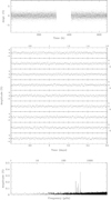 |
Fig. 1 Photometry obtained for Feige 46 (TIC 371813244) with TESS. Top panel: light curve from Sector 22 (amplitude is in percentof the mean brightness of the star) spanning 26.59 d (638.16 h) sampled every 120 s. Gaps in this time series are caused by the mid-sector interruption during data download and measurements removed from the light curve because of a non-optimal quality warning. Middle panel: close-up view of the light curve covering the first nine days, where modulationsare visible. Bottom panel: Lomb-Scargle Periodogram of the light curve up to the Nyquist frequency limit (~ 4167μHz). Significant periodic signal is clearly detected in the 250−500 μHz range. |
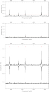 |
Fig. 2 Pre-whitening sequence of detected pulsation modes. Top panel: Lomb-Scargle Periodogram of the TESS time series in the relevant 270−420 μHz frequency range. The horizontal dotted line indicates four times the median noise level and corresponds to the chosen detection limit. Middle panel: residual periodogram after pre-whitening the four dominant peaks identified in the top panel. Two additional low-amplitude peaks are identified. Bottom panel: from top to bottom are the original, reconstructed (from the frequencies, amplitudes, and phases of the six fitted sine waves; plotted upside down) and residual periodograms after completing the pre-whitening process. |
Modes detected in the TESS time series of Feige 46.
3 Parallax, spectral energy distribution, and stellar parameters
The Gaia mission recently provided parallaxes for a large number of hot subdwarf stars. This allows atmospheric parameters to be converted to the fundamental stellar parameters: mass, radius, and luminosity, without relying on predictions from evolutionary models. The parallax measurements for LS IV–14°116 and Feige 46 are of excellent quality, with uncertainties of less than 5%. In addition, photometry is required to derive the angular diameters (θ) of the stars. We combined apparent magnitudes from the ultraviolet to the infrared to construct the observed spectral energy distribution (SED) of LS IV–14°116 (see Fig. 3). Our final synthetic spectrum of LS IV–14°116 was then scaled to fit this SED using χ2 minimisation based on the method described by Heber et al. (2018). Interstellar reddening is considered after Fitzpatrick et al. (2019), assuming an extinction parameter R (55) = 3.02. Fit parameters are the angular diameter θ and E(44−55), which is the monochromatic analogon of the colour excess E(B–V). To derive the stellar radius R, the Gaia parallax ϖ is combined with the resulting angular diameter θ = 2Rϖ. The stellar mass M is then derived using the spectroscopic surface gravity g = GM∕R2, where G is the gravitational constant (log g = 5.85 for LS IV–14°116). The stellar luminosity L is based on the spectroscopic effective temperature (Teff = 35 500 K). We repeated the SED fit for Feige 46 using log g = 5.93 and Teff = 36 100 K (see Fig. E.1). The atmospheric parameters used are the same as those used for the spectroscopic analysis andare described in Sect. 5.1. For both stars, we assume systematic errors of 0.1 dex in log g and 1000 K in Teff. The results of this analysis are listed in Table 2. The derived stellar mass for LS IV–14°116 (0.38 ± 0.10M⊙) is somewhat less than the value obtained for Feige 46 (0.53 ± 0.14M⊙). Given the uncertainties both masses are consistent with the canonical mass suggested by evolution models (~0.46 M⊙, Dorman et al. 1993; Han et al. 2003).
Parallax and parameters derived from the SED fitting.
4 Spectroscopic observations
We obtained four VLT/UVES spectra of Feige 46 in February 2020 with a total exposure time of 5920 s (ID 0104.D-0206(A)). These spectra have a resolution of R ≈ 41 000 and cover the spectral range from 3305 to 6645 Å, with gaps at 4525–4620 Å and 5599–5678 Å. The individual spectra were stacked after cross-correlation to obtain a single spectrum with an increased signal-to-noise ratio (S/N) of about 80. The radial velocity obtained, vrad = 89 km s−1, is fully consistent with the value found by Drilling & Heber (1987): 90 ± 4 km s−1. For the spectral analysis, the observed spectrum was shifted to the stellar rest frame. We refer the reader to Latour et al. (2019b) for the description and analysis of older spectra of Feige 46, including ultraviolet (UV) observations.
LS IV–14°116 has been observed extensively with the UVES spectrograph. A total of 788 spectra are available in the ESO archive (corresponding to 394 exposures). Spectra were taken as part of two programmes: on 7 September, 2011 (ID 087.D-0950(A)) and between 23 and 27 August, 2015 (ID 095.D-0733(A)). These programs used time-resolved spectroscopy in order to relate the observed photometric variability to radial velocity variations (Jeffery et al. 2015; Martin & Jeffery 2017). We combined spectra from both runs to create a high-S/N spectrum that is suitable for a detailed abundance analysis. For each resolution, spectra with the highest S/N (typically 16 to 25) were cross-correlated and stacked. These stacked spectra were convolved to the lowest common resolutions (R = 40 970 for the blue range, and R = 42 310 for the red range) and were then co-added. We then shifted the spectrum to the stellar rest frame, correcting for the high radial velocity of about vrad = −154 km s−1. The final spectrum has a mean effective S/N of about 200, which is limited by small-scale artefacts. Details of the UVES spectra used in the present analysis are given in Table 3.
Randall et al. (2015) carried out spectropolarimetry of LS IV–14°116 with VLT/FORS2 to search for a magnetic field. While no polarisation could be detected, their observations produced a flux spectrum of excellent quality (spectral resolution Δλ ≈ 1.8Å, S∕N ≈ 700). In contrast to the UVES spectra, this long-slit spectrum is not affected by the normalisation issues that frequently occur in the reduction procedure of Echelle spectra. The FORS2 spectrum is therefore useful for determining atmospheric parameters based on broad hydrogen and helium lines.
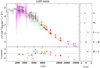 |
Fig. 3 Comparison of smoothed final synthetic spectrum of LS IV–14°116 (grey line) with photometric data. The two black data points labelled “box” are binned fluxes from an IUE spectrum (LWP10814LL, magenta line, Wamsteker et al. 2000). Filter-averaged fluxes are shown as coloured data points that were converted from observed magnitudes (the dashed horizontal lines indicate filter widths). The residual panels at the bottom andon the right sides, respectively, show the differences between synthetic and observed magnitudes/colours. The following colour codes are used to identify the photometric systems: SDSS (yellow, Henden et al. 2015; Alam et al. 2015), SkyMapper (dark yellow, Wolf et al. 2018), Pan-STARRS1 (red, Chambers et al. 2016), Johnson-Cousins (blue, Henden et al. 2015; O’Donoghue et al. 2013), Strömgren (green, Hauck & Mermilliod 1998), Gaia (cyan, Gaia Collaboration 2018), VISTA (dark red, McMahon et al. 2013), DENIS (orange, DENIS Consortium 2005), 2MASS (bright red, Cutri et al. 2003), and WISE (magenta, Schlafly et al. 2019). |
UVES spectra used in the present analysis.
5 Spectroscopic analysis
The excellent UVES spectra enable a detailed abundance analysis, as well as a consistent comparison of abundances between LS IV–14°116 and Feige 46, which is described in the following section.
5.1 Methods
To minimise systematic errors, we analysed the spectra of both Feige 46 and LS IV–14°116 using the same fitting method and the same type of model atmospheres, following the procedure described in Latour et al. (2019b) and Dorsch et al. (2019). This analysis is based on model atmospheres and synthetic spectra computed using the hydrostatic, homogeneous, plane-parallel, non-local thermodynamic equilibrium (NLTE) codes TLUSTY and SYNSPEC (Hubeny 1988; Lanz & Hubeny 2003; Hubeny & Lanz 2011). We used the most recent public versions as described in Hubeny & Lanz (2017a,b,c).
Our line list is based on atomic data provided by R. Kurucz1. We extended this line list to include lines from additional heavy ions. The atomic data previously collected are described in Dorsch et al. (2019) and Latour et al. (2019b). This list was further extended to model the rich spectrum of Feige 46. The main sources for detected lines of heavy ions are listed in Table 4. Heavy elements (here Z > 30) in ionisation stages I-III are included in LTE using the treatment of Proffitt et al. (2001), who added ionisation energies and partition functions from R. Kurucz’s ATLAS9 code (Kurucz 1993) to SYNSPEC. Partition functions for higher ionisation stages are calculated as described in Latour et al. (2019b).
As in our previous analysis of Feige 46, all model atmospheres were calculated using the atmospheric parameters derived by Latour et al. (2019a) (Teff = 36 100 K, log g = 5.93, and a helium abundance of log ɛHe∕ɛH = −0.32). Atmospheric parameters for LS IV–14°116 were derived by Randall et al. (2015) based on a high S/N FORS2 spectrum (Teff = 35 150 K, log g = 5.88, log ɛHe∕ɛH = −0.62). We used a grid of line-blanketed NLTE models to re-fit the same FORS2 spectrum, and we obtained Teff = 35 500 K, log g = 5.85, log ɛHe∕ɛH = −0.60, which is fully compatible with the results of Randall et al. (2015). The model grid used for this fit includes H, He, C, N, O, Ne, Mg, Al, Si, and Fe in NLTE with abundances appropriate for LS IV–14°116.
Using the atmospheric parameters reported above for each star, we then constructed series of models, varying the abundance of one element at a time. These models also include nickel in NLTE. Based on these grids, we determined metal abundances using the χ2 -fitting program SPAS developed by Hirsch (2009).
Both Feige 46 and LS IV–14°116 show slightly broadened lines that are best reproduced at a projected rotational velocity of vrot sini = 9 km s−1. This broadening might not be caused solely by rotation, but instead likely results from unresolved (high-order)pulsations. Indeed, Jeffery et al. (2015) found that the principal pulsation mode in LS IV–14°116 (1950 s) leads to radial velocity variations with a semi-amplitude of about 5.5 km s−1. They also came to the conclusion that other pulsation periods lead to additional unresolved motion. Similar variability could be present in Feige 46, which would explain the observed broadening given that the UVES exposure times (1480 s) cover a significant fraction of the shortest period observed in Feige 46 (2295 s). However, the exposure times of the UVES spectra of LS IV–14°116 were much shorter (200 or 300 s). The remaining broadening (despite cross-correlating individual exposures before co-adding) may be explained by a combination of uncertainties in the cross-correlation, high-order pulsations, unresolved motion due to multiple periods, and actual rotation. Jeffery et al. (2015) also find evidence for differential pulsation: line strength and pulsation amplitude might be correlated. Therefore, correlating single spectra using specific strong lines would not perfectly mitigate the broadening in the stacked spectrum for weak lines. However, differential pulsation was not confirmed in the radial velocity study of Martin & Jeffery (2017). Additional broadening may be caused by microturbulence (vtb). However, as shown by Latour et al. (2019b), a microturbulence of 5 km−1 is too high to simultaneously reproduce UV and optical lines in Feige 46. We therefore adopted vtb = 2 km s−1 for both stars, which leads to negligible broadening.
Sources of oscillator strengths for detected lines of heavy metals in Feige 46 and LS IV–14°116.
5.2 Individual abundances
In the following section, we present, in detail, the result of our abundance analysis for each element. A summary of the abundances derived for Feige 46 and LS IV–14°116 is given in Tables 5 and 6, respectively. Abundances stated in the text are always relative to solar values. The full UVES spectra along with the final models for both stars are shown in Appendix D.
Abundance results for Feige 46 by number relative to hydrogen (log ɛ/ɛH), by number fraction (log ɛ), and number fraction relative to solar (log ɛ/ɛ⊙).
5.2.1 Light elements and the iron group: carbon to zinc
Examples of the strongest lines from light elements for both stars along with the final models are shown in the top panels of Fig. 4. The following paragraphs summarise the derivation of abundances for light metals and the iron group.
Carbon, nitrogen, and oxygen
Plenty of carbon, nitrogen, and oxygen lines are available to determine abundances, including the lines shown in Fig. 4. Both stars have a carbon abundance close to the solar number fraction that is slightly enhanced for Feige 46 (+0.25 dex) and somewhat depleted for LS IV–14°116 (− 0.19 dex). Nitrogen is overabundant in both stars by 0.46 and 0.28 dex, respectively, while oxygen is significantly underabundant by − 1.03 and − 1.23 dex. On average, the CNO content of LS IV–14°116 is lower than that of Feige 46 by about 0.2 dex. Although the general fit for carbon lines is good, there is some discrepancy between the strongest C II and C III lines. We attribute this mostly to NLTE effects that are not perfectly modelled. For instance, the C II 4267.3 Å doublet is too strong in our synthetic spectra, while the C III triplet 4152.5, 4156.5, 4162.9 Å is slightly too weak (see Figs. D.1 and D.2). C II 5661.9 Å is predicted to be in emission although no line is observed at this position in the UVES spectrum of LS IV–14°116. Some nitrogen lines display similar behaviour: N II 4630.5, 4643.1, 4803.3, 5005.2, 5179.5, and 5710.8 Å are too weak in our models and were not considered for determining the nitrogen abundance. These lines also appeared in emission in the synthetic spectra of the iHe-sdO HD 127493 (Dorsch et al. 2019), who used the same model atoms. Resolving these issues is a complex task because almost all optical lines of C II-III and N II originate from high-lying levels. The population of these levels is very sensitive to the photo-ionisation (radiative bound-free) cross-sections used. The development of new TLUSTY model atoms would be required for at least C II-III and N II, which is an elaborate process and beyond of the scope of the present investigation. For the time being, the best fit to lines of C, N, and O can be considered satisfactory. The derived abundances of C, N, and O for Feige 46 do not differ significantly from the values given by Latour et al. (2019b) (see Fig. B.1).
Neon
The slightly sub-solar neon abundance for both stars is based on several Ne II lines in the blue range, for example Ne II 3334.8, 3664.1, and 3694.2 Å.
Magnesium
The Mg II 4481 Å doublet is observed in both stars and best reproduced at abundances of − 0.79 dex for Feige 46, and − 1.07 dex for LS IV–14°116.
Aluminium
The strongest predicted aluminium lines, Al III 4479.9, 4512.6, and 5696.6 Å, are not detected in Feige 46 or LS IV–14°116. The upper limit derived from these lines is slightly sub-solar.
Silicon
Sub-solar silicon abundances are based mainly on the Si IV 4088.9, 4116.1 Å doublet.
Phosphorus
The only phosphorus line observed in Feige 46, P III 4222.2 Å, is very weak but present in LS IV–14°116 as well. The derived abundance based on this line is solar for Feige 46 and slightly sub-solar for LS IV–14°116.
Sulphur
No sulphur lines are detected in either star. The upper limit derived for Feige 46 is consistent with the value found by Latour et al. (2019b) from the UV spectrum.
Argon
The argon abundance for Feige 46 is based on the weak Ar III 3311.6 and 3503.6 Å lines. The same lines could not be used for LS IV–14°116, where the Ar abundance (about solar) is instead based on Ar III 3336.1 and 3511.2 Å. Significant uncertainty (~0.2 dex) is introduced by the continuum placement since all Ar lines are very weak.
Calcium
The upper limits derived for calcium are based on the non-detection of the Ca II 3933.7 Å resonance line, which is well separated from interstellar lines in both stars. These upper limits indicate severe underabundances (by about 0.7 dex) for both stars, which is consistent with the non-detection of the Ca III 4233.7 and 4240.7 Å lines that are usually observed in He-poor sdOB stars.
Titanium
Weak titanium lines are observed in both stars. We used Ti III 3354.7, 4215.5, 4285.6 Å and Ti IV 3541.4, 3576.5, 4971.2, and 5398.9 Å to derive super-solar abundances.
Chromium, manganese, iron, and cobalt
No lines from the iron-peak elements chromium, manganese, iron, and cobalt are observed in UVES spectra of either star. For completeness, we list the abundances derived from UV lines for Feige 46 by Latour et al. (2019b) in Table 5. The absence of high-resolution UV spectra of LS IV–14°116 means that no information on the abundance of these elements can be obtained for that star, except for iron. The iron upper limit for LS IV–14°116 (0.35 times solar) is based on the non-detection of Fe III 5243.3 and 5891.9 Å, which are too strong in the final model. Fe III 4137.8 and 4164.7 Å are well reproduced at this abundance.
Nickel
Several weak nickel lines (Ni III) could be used to derive abundances for both stars, for example Ni III 5332.2, 5436.9, 5481.3 and 5482.3 Å. The Ni abundance derived from the optical lines for Feige 46 is the same as that obtained from the UV lines: overabundant by about 1 dex with respect to solar.
Zinc
The zinc abundances for Feige 46 and LS IV–14°116 (about 300 times solar) are based on 13 and 16 strong lines, respectively (e.g. Zn III 3683.4, 4818.9, 4970.8, 5075.2, 5249.7, and 5563.7 Å; see Fig. 4).
5.2.2 Heavy metals
From a spectroscopic perspective, the prevalence of strong lines of heavy elements (here Z > 30) is the most striking feature of LSIV–14°116 and Feige 46. Nevertheless, many lines of heavy metals remained either undetected in the previous analyses (Naslim et al. 2011; Latour et al. 2019b), owing to the limited S/N and wavelength coverage of the spectra available, or unidentified due to the scarcity of atomic data. Therefore, we set out to identify these lines that are present both in LS IV–14°116 and Feige 46.
Oscillator strengths are available for many ions that are expected to show spectral lines in the programme stars. However, several of these lines have remained unidentified so far because their rest wavelengths are not known with sufficient precision. The large wavelength coverage and good S/N of our spectra allowed us to identify lines of such ions from predicted relative intensities by adjusting the theoretical wavelengths to match the position of observed lines. These empirical wavelengths may also be useful in future atomic structure calculations.
The 102 detected heavy-metal lines with available oscillator strengths are listed in Table C.1. This includes strong previously unidentified lines noted by Naslim et al. (2011) at 4007 and 4216 Å, that now appear to be Sr III and Sn IV. Lines that required significant shifts to match observed lines are additionally listed in Table 7. The 21 newly identified lines that lack oscillator strengths are listed in Table C.2; some are shown in Fig. 5. The 51 remaining unidentified lines are listed in Table C.3. In the following paragraphs, we briefly describe the analysis for each heavy element detected. The strongest modelled lines for each heavy element are shown in Fig. 4 (Ga, Y, Sn, Pb), Fig. 6 (Ge, Kr, Sr), and Fig. 7 (Zr) for both stars.
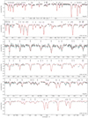 |
Fig. 4 Representative regions in the UVES spectra of Feige 46 and LS IV–14°116. The best fit models are shown in red. |
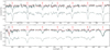 |
Fig. 5 Additional regions in the UVES spectrum of Feige 46 showing newly identified lines that are lacking oscillator strengths and the strongest unidentified line observed. The UVES spectrum of LS IV–14°116 is shown for comparison, offset by − 0.1. |
Gallium
We identified several Ga III lines in the spectra of Feige 46 and LS IV–14°116. Oscillator strengths for optical Ga III lines were derived by O’Reilly & Dunne (1998). In particular, Ga III 3517.4, 3577.3, 3806.7, 4380.6, 4381.8, 4993.9, 5337.2, 5358.2, 5844.9, and 5993.9 Å could be used to derive an abundance of about 2000 times solar for both stars. To our knowledge, they have never been observed in any star.
Germanium
Naslim et al. (2011) identified and provide oscillator strengths for three Ge III lines in the optical spectrum of LS IV–14°116. Oscillator strengths for optical lines of Ge IV were provided by O’Reilly & Dunne (1998). However, these Ge IV lines have never been used to derive abundances, and their wavelengths had to be shifted to match the observed ones as listed in Table 7. We used these three Ge III lines as well as four Ge IV lines to derive a germanium abundance of 2000 times solar for both stars. There is a mismatch between Ge III and Ge IV lines, which systematically appear too weak in our synthetic spectra. This may be due to NLTE effects or systematic differences between the atomic data used for Ge III and Ge IV.
An effective temperature of 35 920 K would be required for LS IV–14°116 to simultaneously reproduce both ionisation stages. However, this temperature is too high by about 400 K to be able to reproduce the ionisation balance of most other elements.
Updated line positions.
Arsenic
Two weak, unidentified lines at 3922.5 and 4037 Å are observed close to experimental wavelengths of the As III lines provided by Lang (1928), as listed in NIST2. We are not aware of oscillator strengths for optical As III lines, and, therefore, cannot derive the abundance.
Selenium
Fifteen previously unidentified lines were identified with Se III using the experimental wavelengths provided by Badami & Rao (1933) as listed in NIST (see Fig. 5). This is the first time these lines have been observed in any star, and they are visible in both Feige 46 and LS IV–14°116. A list of identifications is given in Table C.2. Unfortunately, no oscillator strengths are available for optical Se III lines.
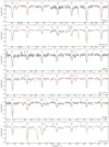 |
Fig. 6 Strongest lines identified in the UVES spectra of Feige 46 and LS IV–14°116 for elements Ge, Kr, and Sr. |
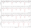 |
Fig. 7 Zr IV lines and one Zr III line identified in UVES spectra of Feige 46 and LS IV–14°116 at the best fit abundances. |
Krypton
Kr III shows many lines in the UVES spectra of Feige 46 and LS IV–14°116 that have never been identified in any star as far as we know3. Fortunately,oscillator strengths are provided by Raineri et al. (1998) allowing us to determine the krypton abundance. Some lines were shifted to match the observed position; they are listed in Table 7. We have used Kr III 3325.76, 3342.48, 3351.94, 3474.65, 3488.55, 3564.24, 3641.35, 3690.66, and 4067.40 Å to derive an abundance of about 5500 times solar for both stars. The predicted Kr III 3308.22, 3396.72 Å lines do not match observed lines. The alternative oscillator strengths for these two lines provided by Eser & Özdemir (2018) are even larger. These lines might require large shifts or have inaccurate oscillator strengths.
Strontium
In total, 35 previously unidentified lines can clearly be attributed to Sr III: for example, the strong 3430.8, 3936.4 Å lines. To our knowledge, these lines have never before been reported in stellar spectra. Wavelengths and oscillator strengths for Sr II-III were provided by R. Kurucz, allowing us to determine the strontium abundance. The resonance lines Sr II 4077.7, 4215.5 Å used by Naslim et al. (2011) to derive the strontium abundance in LS IV–14°116 are also observed in Feige 46. To model these lines, we used oscillator strengths from Fernández-Menchero et al. (2020), who recently investigated Sr II in detail (along with Y III and Zr IV). Both stars also show Sr II lines at 3380.7, 3464.5, and 4305.4 Å. Fitting four Sr II lines (three for Feige 46) as well as 21 Sr III lines (19 for Feige 46) results in an abundance of 43 000 times solar for LS IV–14°116 and 31 000 times solar for Feige 46.
Yttrium
Naslim et al. (2011) identified two strong yttrium lines in the spectrum of LS IV–14°116: Y III 4039.602 and 4040.112 Å. Fitting these lines (Y III 4039.6 Å at a slightly revised position) results in abundances of 27 000 times solar for Feige 46 and 40 000 times solar for LS IV–14°116. Oscillator strengths for additional Y III lines observed at 5102.9, 5238.1, and 5602.2 Å are provided by Fernández-Menchero et al. (2020). However, these lines are not consistent with Y III 4039.6, 4040.1 Å and were therefore not considered for the abundance determination.
 |
Fig. 8 Abundance patterns of LS IV–14°116 and Feige 46 relative to that of the Sun (by number fraction). Only elements with an abundance measurement are shown. Upper limits are marked with an arrow and less saturated colours. For comparison, abundance measurements for He-poor sdOB stars (33000 K < Teff < 36500 K) are shown as grey open circles (Geier 2013, based on optical data), diamonds (Chayer et al. 2006, based on far-UV data), and squares (O’Toole & Heber 2006, based on UV data). |
Zirconium
By far the strongest lines from heavy metals in the optical spectrum of both stars originate from zirconium IV transitions (see Fig. 7). Oscillator strengths for four Zr IV lines were provided by Naslim et al. (2011) and for two additional lines by Naslim et al. (2013). Rauch et al. (2017) also provide oscillator strengths for a large number of UV and optical Zr IV lines, while Fernández-Menchero et al. (2020) have recently computed oscillator strengths for eight Zr IV lines that are observed in the UVES spectra of both stars. We exclusively rely on data from Rauch et al. (2017), as they provide the most extensive list. A single strong Zr III line is observed at 3497.9 Å and is somewhat too weak in our models. We used this line as well as several Zr IV lines to determine the abundance in both stars, including the four Zr IV lines used by Naslim et al. (2011). The best fit Zr abundance for LS IV–14°116, 40 000 times solar, is significantly higher than that for Feige 46 (20 000 times solar). As shown in Fig. 7, Zr IV lines are very well reproduced in both stars (with the exception of Zr IV 3919.3 and 5462.3 Å, which are too strong in our models). In addition, we slightly revised the position of two Zr IV lines: Zr IV 5462.38 and 5779.88 Å.
Tin
Strong spectral lines of Sn IV at 3862.1 and 4217.2 Å are visible in the UVES spectra of Feige 46 and LS IV–14°116. These lines have not been previously identified in any star. To model these lines, we used oscillator strengths provided by Kaur et al. (2020), but the rest wavelengths had to be adjusted (see Table 7). The abundance of tin derived from the two newly identified lines turns out to be 22 000 times solar for LS IV–14°116 and 3700 times solar for Feige 46, which is consistent with the value derived from UV lines by Latour et al. (2019b).
Lead
The lead abundance of LS IV–14°116, 2800 times solar, is based on a very weak Pb IV 4049.8 Å line. No other lead lines are detected, thus the abundance has a large uncertainty. Latour et al. (2019b) determined an upper limit for lead in Feige 46, 680 times solar. It is based on the Pb IV 1313 Å resonance line and is likely close to the actual abundance. Although this upper limit is consistent with the non-detection of Pb lines in the optical spectrum of Feige 46, it should be confirmed by UV observations of higher quality than the low S/N IUE spectrum that is currently available.
Undetected elements
We searched unsuccessfully for lines of fluorine, sodium, chlorine, potassium, scandium, vanadium, rubidium, and xenon. Details can be found in Appendix A.
5.3 The emerging abundance pattern
Both stars show almost the same abundance pattern, as illustrated in Fig. 8. When compared to solar values, nitrogen is enhanced and oxygen depleted. Carbon is slightly super-solar in Feige 46 and slightly sub-solar in LS IV–14°116. The light metals C, N, O, Ne, Mg, Si, and P are all slightly more abundant in Feige 46, but otherwise follow the same pattern as in LS IV–14°116. The abundances of elements from argon to krypton (when known) are almost identical, and calcium is depleted in both stars. Heavy elements are enriched to very high values, from zinc at about 300 times solar, to zirconium well above 20 000 times solar. While being highly enriched when compared to solar values, the concentration of Sr, Y, Zr, Sn, and Pb in the line-forming region of Feige 46 is progressively less extreme when compared to that of LS IV–14°116. This enrichment is nevertheless notable when compared to He-poor sdOB stars, which have been observed to be enhanced inZn, Ga, Ge, Zr, and Sn to about 10 to 200 times the solar value (O’Toole & Heber 2006; Chayer et al. 2006; Blanchette et al. 2008). The extreme enrichment in heavy metals and the abundances of lighter metals are different to those observed in He-poor sdOB stars. In particular, the argon and calcium abundances in LS IV–14°116 and Feige 46 aresignificantly lower than the super-solar values Geier (2013) obtained for He-poor sdOBs of similar temperatures.
Such strong deficiency when compared to He-poor sdOB stars (2 dex for calcuium) cannot be explained by a lower initial metallicity that might be expected for LS IV–14°116 and Feige 46 due to their halo kinematics. It is worth mentioning that this calcium deficiency is not observed in lead-rich iHe-sdOB stars such as [CW83] 0825+15 (Jeffery et al. 2017a), FBS 1749+373, and PG 1559+048 (Naslim et al. 2020). These stars show calcium abundances in line with those observed in He-poor sdOB stars. In contrast to this, the carbon and nitrogen abundances in LS IV–14°116 and Feige 46 are higher than in the average He-poor sdOB star. Such enrichment could be caused by an excess of material processed by H-burning (CNO-cycle) and He-burning (3α) in the atmospheres of LS IV–14°116 and Feige 46 when compared to He-poor sdOB stars, as predicted for both hot flasher (Miller Bertolami et al. 2008) and merger scenarios (Zhang & Jeffery 2012). This is consistent with the positive correlation between the helium and carbon abundances of sdOB stars in the globular cluster ω Cen, as found by Latour et al. (2014). In addition, the abundances of C, N, and O might still be affected by diffusion processes to some degree (in both He-poor and iHe-sdOB stars).
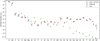 |
Fig. 9 Atmospheric abundances for LS IV–14°116 and Feige 46 by number fraction (with solar values from Asplund et al. 2009). |
6 Discussion and conclusions
We performed a detailed spectral analysis of Feige 46 and LS IV–14°116. This consistent analysis of both stars enables an accurate and direct comparison of their abundance patterns, which would be hampered by the use of different analysis methods.
The abundance patterns of both stars, as well as their differences, can likely be explained with atmospheric diffusion processes. In terms of diffusion, it is convenient to consider the abundance pattern as number fraction without the comparison to solar values (Fig. 9). It is easy to recognise that, overall, the abundance of light metals from carbon to phosphor drops by three orders of magnitude from log ɛ ≈−3.5 to about −6.5 dex. Unlike in the Sun, the abundances of heavier elements (except calcium) do not continue to drop further, but follow a more constant pattern. A comparison of detailed diffusion calculations with these observed abundance patterns is required to resolve the question of whether diffusion alone is enough to produce such high enrichment of heavy metals. In addition, atmospheric models that consider atmospheric stratification are required to determine whether the observed heavy-metal enrichment can be explained by thin layers of enriched material in the line-forming region.
Thanks to the excellent quality and wavelength coverage, we were able to identify many previously unidentified lines in the UVES spectra of Feige 46 and LS IV–14°116 with transitions of heavy ions. Strong lines with available oscillator strengths originate from ions such as Ge IV, Kr III, Sr III, Zr III, and Sn IV. Their identification will enable the determination of abundances in future analyses of other heavy-metal stars, even with spectra of lower quality. Atomic data are still lacking for some heavy elements and ionisation stages III-IV, including several newly identified lines of Ge III, Se III, and Y III. We also provide observed wavelengths for these lines that may be useful in future atomic structure calculations. About 50, mostly weak, lines detected in the spectra of LS IV–14°116 and Feige 46 remain unidentified and could belong to elements not yet identified in either star.
We also analysed the TESS light curve of Feige 46 and detected five of the six modes found by Latour et al. (2019a). The period stability of these five pulsation modes (Ṗ ≲ 10−8 s s−1) is not compatible with the stronger period decay predicted by Battich et al. (2018) for a star quickly evolving through a series of late helium flashes. This questions the idea that Feige 46 may be a pre-EHB object with pulsations driven by the ɛ-mechanism generated by late helium flashes.
Stellar parameters (mass, radius, and luminosity) were derived from the high-quality Gaia parallax by combining it with the atmospheric parameters and the spectral energy distribution. The results for both stars are limited by the uncertainty of the surface gravity, but consistent with the canonical subdwarf mass predicted by hot flasher models (0.46 M⊙, Dorman et al. 1993; Han et al. 2003).
The similarity of LS IV–14°116 and Feige 46 in terms of atmospheric parameters, abundances, pulsation, and kinematics remains puzzling. A larger sample of intermediately He-rich sdOB stars with detailed observed abundance patterns is required to draw conclusions regarding the causal relation between these features. Such a sample would also be required in order to answer the questions:
-
What makes the heavy-metal stars different from the normal sdOB stars? Other chemically peculiar stars such as helium-rich main-sequence B stars and Ap stars have strong magnetic fields, and so it has been suggested that the heavy-metal stars are magnetic too, but no magnetic field has been detected in LS IV-14 116 (down to 300 G, Randall et al. 2015).
-
Are most iHe-sdOB stars an intermediate stage in the evolution of He-sdOs towards the He-poor sdBs?
-
At which point in their evolution will atmospheric diffusion become important?
Fortunately, recent surveys such as the LAMOST survey (e.g. Lei et al. 2020) and the SALT/HRS survey (e.g. Jeffery et al. 2017b) are discovering many new He-rich subdwarf stars. Future analyses of a larger sample of stars that share the atmospheric parameters of LS IV–14°116 and Feige 46 (intermediate He-enrichment and Teff around 35 000 K), but also of their possible progenitors, the extreme He-sdOs, might give important clues towards the evolution of He-rich subdwarf stars.
Acknowledgements
We thank Simon Kreuzer for the development of the photometry query tool and Ingrid Pelisoli for very helpful comments on TESS. We thank the referee, Suzanna Randall, for useful suggestions that improved this paper. M.L. acknowledges funding from the Deutsche Forschungsgemeinschaft (grant DR 281/35-1). S.C. acknowledges financial support from the Centre National d’Études Spatiales (CNES, France) and from the Agence Nationale de la Recherche (ANR, France) under grant ANR-17-CE31-0018. Based on observations collected at the European Southern Observatory under ESO programmes 0104.D-0206(A), 087.D-0950(A), and 095.D-0733(A). This paper includes data collected by the TESS mission, which are publicly available from the Mikulski Archive for Space Telescopes (MAST). Funding for the TESS mission is provided by NASA’s Science Mission directorate. Based on INES data from the IUE satellite. This work has made use of data from the European Space Agency (ESA) mission Gaia (https://www.cosmos.esa.int/gaia), processed by the Gaia Data Processing and Analysis Consortium (DPAC, https://www.cosmos.esa.int/web/gaia/dpac/consortium). Funding for the DPAC has been provided by national institutions, in particular the institutions participating in the Gaia Multilateral Agreement. Based on observations obtained as part of the VISTA Hemisphere Survey, ESO Progam, 179.A-2010 (PI: McMahon). The TOSS service (http://dc.g-vo.org/TOSS) used for this paper was constructed as part of the activities of the German Astrophysical Virtual Observatory. We acknowledge the use of the Atomic Line List (http://www.pa.uky.edu/ peter/newpage/). This research has made use of NASA’s Astrophysics Data System.
Appendix A Additional elements investigated
In the following, we describe additional elements that could not be detected in Feige 46 and LS IV–14°116. Upper limits are listed in Table A.1. As in Tables 5 and 6, upper limits are given as best fit values, while their uncertainties represent values that can clearly be excluded.
Upper limits for elements that could not be detected.
F II 3505.6, 3847.1, 3850.0, and 4246.2 Å exclude abundances higher than about 100 times solar in LS IV–14°116. The very weak photospheric resonance lines Na I 5889.94 and 5889.96 Å are well separated from the interstellar lines, but unfortunately blended with the stronger C II 5889.78 Å. These lines, as well as Na II 3533.1 Å, seem to exclude abundances higher than about five times solar in LS IV–14°116, while no sensible upper limit can be derived for Feige 46. Chlorine abundances higher than six times solar for Feige 46 and about four times solar for LS IV–14°116 can be excluded based on the non-detection of Cl III 3530.0, 3601.9 Å.
The upper limits derived for the following elements are either too high to be of use, or uncertain because of poorly known line positions. We therefore refrain from stating even an upper limit.
K II 4186.2 Å seems to fit a weak line in LS IV–14°116 at an abundance of about 30 times solar. However, this abundance seems to be excluded by K III 3322.4, 3358.4, and 3364.3 Å, which suggest an upper limit of about ten times solar. The upper limit derived from the non-detection of very weak predicted Sc III and V III lines are next to meaningless for both stars. Zhang et al. (2014) provided atomic data for Rb III. However, because these lines have never been observed, their positions are likely not accurate. They do not match observed lines in Feige 46 or LS IV–14°116. The same is true for optical Xe IV lines as predicted by Rauch et al. (2017).
Appendix B Comparison with abundances from Latour et al. (2019b)
Our results for Feige 46 are in good agreement with the abundances derived by Latour et al. (2019b). The excellent agreement for Ti, Ni, Zn, Ga, Sr, and Sn is remarkable because these abundances were previously solely based on UV data. The slight disagreement for Si and Ge may be explained with the low S/N of the CASPEC and IUE spectra used by Latour et al. (2019b).
 |
Fig. B.1 Comparison with results from Latour et al. (2019b). |
Appendix C Observed wavelengths
Table C.1 lists all detected lines from heavy elements for which oscillator strengths are available. Since observed wavelengths are useful in the calculation of oscillator strengths, we also list in Table C.2 observed positions forlines that could be identified but do not have oscillator strengths available.
Several, mostly weak, lines are visible in the UVES spectra of both Feige 46 and LS IV–14°116, but they remain unidentified. They are listed in Table C.3. These lines are visible in both stars and therefore likely to be real. They might be due to transitions in heavy ions.
Identified lines of heavy metals (Z > 30) in the UVES spectra of LS IV–14°116 and Feige 46 for which oscillator strengths are available.
Observed wavelengths for newly identified lines that lack oscillator strengths in the spectra of LS IV–14°116 and Feige 46.
Remaining unidentified lines in the spectra of LS IV–14°116 and Feige 46.
Appendix D Full spectral comparisons
This section presents the full spectral comparison between the co-added UVES spectra of LS IV–14°116 and Feige 46 and our final synthetic spectra. The observations have been shifted to laboratory wavelengths and normalised to match the continuum levels of our synthetic spectra. The synthetic spectra are convolved with a variable Gaussian kernel for a resolution of R = 40 970. Rotational broadening was considered at vrot sini = 9 km s−1 using the auxiliary program, ROTIN3, delivered with SYNSPEC and a limb-darkening coefficient of 0.3 (which is more appropriate for compact stars than the default of 0.6). The strongest photospheric metal lines are labelled in black, while identified lines for which no oscillator strengths are available are labelled in red.
 |
Fig. D.1 UVES spectrum of Feige 46 (grey) and final model (red). |
 |
Fig. D.1 continued. |
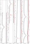 |
Fig. D.1 continued. |
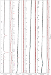 |
Fig. D.1 continued. |
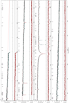 |
Fig. D.1 continued. |
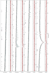 |
Fig. D.1 continued. |
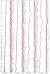 |
Fig. D.2 UVES spectrum of LS IV–14°116 (grey) and final model (red). |
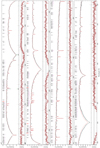 |
Fig. D.2 continued. |
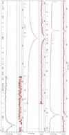 |
Fig. D.2 continued. |
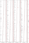 |
Fig. D.2 continued. |
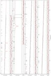 |
Fig. D.2 continued. |
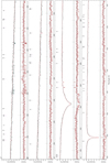 |
Fig. D.2 continued. |
Appendix E SED of Feige 46
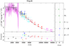 |
Fig. E.1 Same as Fig. 3 but for Feige 46. The following colour codes are used to identify the photometric systems: SDSS (yellow, Henden et al. 2015), Pan-STARRS1 (red, Chambers et al. 2016), Johnson-Cousins (blue, Mermilliod 1994; Henden et al. 2015), Strömgren (green, Hauck & Mermilliod 1998), Gaia (cyan, Gaia Collaboration 2018), UKIDSS (rose, Lawrence et al. 2007), 2MASS (bright red, Cutri et al. 2003), and WISE (magenta, Schlafly et al. 2019). Three IUE spectra were used to construct the box filters (SWP17466RL, SWP20342L, LWR16264LL). |
References
- Ahmad, A., & Jeffery, C. S. 2005, A&A, 437, L51 [NASA ADS] [CrossRef] [EDP Sciences] [Google Scholar]
- Alam, S., Albareti, F. D., Allende Prieto, C., et al. 2015, ApJS, 219, 12 [NASA ADS] [CrossRef] [Google Scholar]
- Asplund, M., Grevesse, N., Sauval, A. J., & Scott, P. 2009, ARA&A, 47, 481 [NASA ADS] [CrossRef] [Google Scholar]
- Badami, J. S., & Rao, K. R. 1933, Proc. R. Soc. London Ser. A, 140, 387 [CrossRef] [Google Scholar]
- Battich, T., Bertolami, M. M. M., Córsico, A. H., & Althaus, L. G. 2018, A&A, 614, A136 [NASA ADS] [CrossRef] [EDP Sciences] [Google Scholar]
- Billéres, M., Fontaine, G., Brassard, P., et al. 2000, ApJ, 530, 441 [NASA ADS] [CrossRef] [Google Scholar]
- Blanchette, J.-P., Chayer, P., Wesemael, F., et al. 2008, ApJ, 678, 1329 [NASA ADS] [CrossRef] [Google Scholar]
- Chambers, K. C., Magnier, E. A., Metcalfe, N., et al. 2016, ArXiv e-prints [arXiv:1612.05560] [Google Scholar]
- Charpinet, S., Fontaine, G., Brassard, P., & Dorman, B. 1996, ApJ, 471, L103 [NASA ADS] [CrossRef] [PubMed] [Google Scholar]
- Charpinet, S., Fontaine, G., Brassard, P., et al. 1997, ApJ, 483, L123 [NASA ADS] [CrossRef] [PubMed] [Google Scholar]
- Charpinet, S., Green, E. M., Baglin, A., et al. 2010, A&A, 516, L6 [NASA ADS] [CrossRef] [EDP Sciences] [Google Scholar]
- Chayer, P., Fontaine, M., Fontaine, G., Wesemael, F., & Dupuis, J. 2006, Balt. Astron., 15, 131 [NASA ADS] [Google Scholar]
- Cutri, R. M., Skrutskie, M. F., van Dyk, S., et al. 2003, VizieR Online Data Catalog: II/246 [Google Scholar]
- DENIS Consortium 2005, VizieR Online Data Catalog: The DENIS database [Google Scholar]
- Dorman, B., Rood, R. T., & O’Connell, R. W. 1993, ApJ, 419, 596 [CrossRef] [Google Scholar]
- Dorsch, M., Latour, M., & Heber, U. 2019, A&A, 630, A130 [NASA ADS] [CrossRef] [EDP Sciences] [Google Scholar]
- Drilling, J. S., & Heber, U. 1987, Second Conference on Faint Blue Stars, eds. A. G. D. Philip, D. S. Hayes, & J. W. Liebert, IAU Colloq., 95, 603 [Google Scholar]
- Eser, S., & Özdemir, L. 2018, Can. J. Phys., 96, 664 [CrossRef] [Google Scholar]
- Fernández-Menchero, L., Jeffery, C. S., Ramsbottom, C. A., & Ballance, C. P. 2020, MNRAS, 496, 2558 [CrossRef] [Google Scholar]
- Fitzpatrick, E. L., Massa, D., Gordon, K. D., Bohlin, R., & Clayton, G. C. 2019, ApJ, 886, 108 [NASA ADS] [CrossRef] [Google Scholar]
- Fontaine, G., Green, E., Brassard, P., Latour, M., & Chayer, P. 2014, ASP Conf. Ser., 481, 83 [Google Scholar]
- Gaia Collaboration 2018, VizieR Online Data Catalog: I/345 [Google Scholar]
- Geier, S. 2013, A&A, 549, A110 [NASA ADS] [CrossRef] [EDP Sciences] [Google Scholar]
- Green, E. M., Fontaine, G., Reed, M. D., et al. 2003, ApJ, 583, L31 [NASA ADS] [CrossRef] [Google Scholar]
- Green, E. M., Guvenen, B., O’Malley, C. J., et al. 2011, ApJ, 734, 59 [NASA ADS] [CrossRef] [Google Scholar]
- Groth, H. G., Kudritzki, R. P., & Heber, U. 1985, A&A, 152, 107 [NASA ADS] [Google Scholar]
- Han, Z., Podsiadlowski, P., Maxted, P. F. L., & Marsh, T. R. 2003, MNRAS, 341, 669 [NASA ADS] [CrossRef] [Google Scholar]
- Hauck, B., & Mermilliod, M. 1998, A&AS, 129, 431 [NASA ADS] [CrossRef] [EDP Sciences] [Google Scholar]
- Heber, U. 2009, ARA&A, 47, 211 [NASA ADS] [CrossRef] [Google Scholar]
- Heber, U. 2016, PASP, 128, 082001 [NASA ADS] [CrossRef] [Google Scholar]
- Heber, U., Irrgang, A., & Schaffenroth, J. 2018, Open Astron., 27, 35 [Google Scholar]
- Henden, A. A., Levine, S., Terrell, D., & Welch, D. L. 2015, AAS Meeting Abstracts, 225, 336.16 [Google Scholar]
- Hirsch, H. A. 2009, PhD thesis, Friedrich-Alexander University Erlangen-Nürnberg [Google Scholar]
- Holdsworth, D. L., Østensen, R. H., Smalley, B., & Telting, J. H. 2017, MNRAS, 466, 5020 [Google Scholar]
- Hu, H., Tout, C. A., Glebbeek, E., & Dupret, M.-A. 2011, MNRAS, 418, 195 [NASA ADS] [CrossRef] [Google Scholar]
- Hubeny, I. 1988, Comput. Phys. Commun., 52, 103 [NASA ADS] [CrossRef] [Google Scholar]
- Hubeny, I., & Lanz, T. 2011, Astrophysics Source Code Library [record ascl:1109.021] [Google Scholar]
- Hubeny, I., & Lanz, T. 2017a, ArXiv e-prints [arXiv:1706.01859] [Google Scholar]
- Hubeny, I., & Lanz, T. 2017b, ArXiv e-prints [arXiv:1706.01935] [Google Scholar]
- Hubeny, I., & Lanz, T. 2017c, ArXiv e-prints [arXiv:1706.01937] [Google Scholar]
- Jeffery, C. S. 2011, Inf. Bull. Variable Stars, 5964, 1 [Google Scholar]
- Jeffery, C. S., & Miszalski, B. 2019, MNRAS, 489, 1481 [Google Scholar]
- Jeffery, C. S., & Saio, H. 2006, MNRAS, 372, L48 [NASA ADS] [CrossRef] [Google Scholar]
- Jeffery, C. S., Pereira, C., Naslim, N., & Behara, N. 2012, ASP Conf. Ser., 452, 41 [Google Scholar]
- Jeffery, C. S., Ahmad, A., Naslim, N., & Kerzendorf, W. 2015, MNRAS, 446, 1889 [NASA ADS] [CrossRef] [Google Scholar]
- Jeffery, C. S., Baran, A. S., Behara, N. T., et al. 2017a, MNRAS, 465, 3101 [NASA ADS] [CrossRef] [Google Scholar]
- Jeffery, C. S., Neelamkodan, N., Woolf, V. M., Crawford, S. M., & Østensen, R. H. 2017b, Open Astron., 26, 202 [CrossRef] [Google Scholar]
- Kaur, M., Nakra, R., Arora, B., Li, C.-B., & Sahoo, B. K. 2020, J. Phys. B At. Mol. Phys., 53, 065002 [CrossRef] [Google Scholar]
- Kramida, A., Yu, R., Reader, J., & NIST ASD Team 2019, NIST Atomic Spectra Database (ver. 5.7.1), Available: http://physics.nist.gov/asd [2020, May 28], National Institute of Standards and Technology, Gaithersburg, MD [Google Scholar]
- Kurucz, R. 1993, ATLAS9 Stellar Atmosphere Programs and 2 km/s grid, Kurucz CD-ROM No. 13. Cambridge, 13 [Google Scholar]
- Kurucz, R. L. 2018, ASP Conf. Ser., 515, 47 [NASA ADS] [Google Scholar]
- Lang, R. J. 1928, Phys. Rev., 32, 737 [CrossRef] [Google Scholar]
- Lanz, T., & Hubeny, I. 2003, ApJS, 146, 417 [NASA ADS] [CrossRef] [Google Scholar]
- Latour, M., Randall, S. K., Fontaine, G., et al. 2014, ApJ, 795, 106 [NASA ADS] [CrossRef] [Google Scholar]
- Latour, M., Green, E. M., & Fontaine, G. 2019a, A&A, 623, L12 [NASA ADS] [CrossRef] [EDP Sciences] [Google Scholar]
- Latour, M., Dorsch, M., & Heber, U. 2019b, A&A, 629, A148 [NASA ADS] [CrossRef] [EDP Sciences] [Google Scholar]
- Lawrence, A., Warren, S. J., Almaini, O., et al. 2007, MNRAS, 379, 1599 [NASA ADS] [CrossRef] [MathSciNet] [Google Scholar]
- Lei, Z., Zhao, J., Németh, P., & Zhao, G. 2020, ApJ, 889, 117 [NASA ADS] [CrossRef] [Google Scholar]
- Martin, P., & Jeffery, C. S. 2017, Open Astron., 26, 240 [NASA ADS] [CrossRef] [Google Scholar]
- Martin, P., Jeffery, C. S., Naslim, N., & Woolf, V. M. 2017, MNRAS, 467, 68 [NASA ADS] [Google Scholar]
- McMahon, R. G., Banerji, M., Gonzalez, E., et al. 2013, The Messenger, 154, 35 [NASA ADS] [Google Scholar]
- Mermilliod, J. C. 1994, VizieR Online Data Catalog: II/193 [Google Scholar]
- Michaud, G., Richer, J., & Richard, O. 2011, A&A, 529, A60 [NASA ADS] [CrossRef] [EDP Sciences] [Google Scholar]
- Miller Bertolami, M. M., Althaus, L. G., Unglaub, K., & Weiss, A. 2008, A&A, 491, 253 [NASA ADS] [CrossRef] [EDP Sciences] [Google Scholar]
- Miller Bertolami, M. M., Córsico, A. H., & Althaus, L. G. 2011, ApJ, 741, L3 [NASA ADS] [CrossRef] [Google Scholar]
- Miller Bertolami, M. M., Battich, T., Corsico, A. H., Christensen-Dalsgaard, J., & Althaus, L. G. 2020, Nat. Astron. 4, 67 [CrossRef] [Google Scholar]
- Naslim, N., Jeffery, C. S., Behara, N. T., & Hibbert, A. 2011, MNRAS, 412, 363 [NASA ADS] [CrossRef] [Google Scholar]
- Naslim, N., Jeffery, C. S., Hibbert, A., & Behara, N. T. 2013, MNRAS, 434, 1920 [NASA ADS] [CrossRef] [Google Scholar]
- Naslim, N., Jeffery, C. S., & Woolf, V. M. 2020, MNRAS, 491, 874 [Google Scholar]
- Németh, P., Kawka, A., & Vennes, S. 2012, MNRAS, 427, 2180 [NASA ADS] [CrossRef] [Google Scholar]
- O’Donoghue, D., Kilkenny, D., Koen, C., et al. 2013, MNRAS, 431, 240 [NASA ADS] [CrossRef] [Google Scholar]
- O’Reilly, F., & Dunne, P. 1998, J. Phys. B At. Mol. Phys., 31, 1059 [NASA ADS] [CrossRef] [Google Scholar]
- O’Toole, S. J., & Heber, U. 2006, A&A, 452, 579 [NASA ADS] [CrossRef] [EDP Sciences] [Google Scholar]
- Proffitt, C. R., Sansonetti, C. J., & Reader, J. 2001, ApJ, 557, 320 [NASA ADS] [CrossRef] [Google Scholar]
- Raineri, M., Reyna Almandos, J. G., Bredice, F., et al. 1998, J. Quant. Spectr. Rad. Transf., 60, 25 [CrossRef] [Google Scholar]
- Randall, S. K., Bagnulo, S., Ziegerer, E., Geier, S., & Fontaine, G. 2015, A&A, 576, A65 [NASA ADS] [CrossRef] [EDP Sciences] [Google Scholar]
- Rauch, T., Gamrath, S., Quinet, P., et al. 2017, A&A, 599, A142 [NASA ADS] [CrossRef] [EDP Sciences] [Google Scholar]
- Reed, M. D., Baran, A. S., Telting, J. H., et al. 2018, Open Astron., 27, 157 [NASA ADS] [CrossRef] [Google Scholar]
- Safronova, U. I., & Johnson, W. R. 2004, Phys. Rev. A, 69, 052511 [NASA ADS] [CrossRef] [Google Scholar]
- Saio, H., & Jeffery, C. S. 2019, MNRAS, 482, 758 [NASA ADS] [CrossRef] [Google Scholar]
- Schlafly, E. F., Meisner, A. M., & Green, G. M. 2019, ApJS, 240, 30 [Google Scholar]
- Stroeer, A., Heber, U., Lisker, T., et al. 2007, A&A, 462, 269 [NASA ADS] [CrossRef] [EDP Sciences] [Google Scholar]
- Sweigart, A. V. 1987, ApJS, 65, 95 [NASA ADS] [CrossRef] [Google Scholar]
- Wamsteker, W., Skillen, I., Ponz, J., et al. 2000, Astrophys. Space Sci., 273, 155 [NASA ADS] [CrossRef] [Google Scholar]
- Wolf, C., Onken, C. A., Luvaul, L. C., et al. 2018, PASA, 35, e010 [Google Scholar]
- Zhang, X., & Jeffery, C. S. 2012, MNRAS, 419, 452 [NASA ADS] [CrossRef] [Google Scholar]
- Zhang, W., Palmeri, P., & Quinet, P. 2014, Eur. Phys. J. D, 68, 104 [CrossRef] [EDP Sciences] [Google Scholar]
- Zong, W., Charpinet, S., & Vauclair, G. 2016, A&A, 594, A46 [NASA ADS] [CrossRef] [EDP Sciences] [Google Scholar]
National Institute of Standards and Technology, https://physics.nist.gov/PhysRefData/ASD/lines_form.html; see also Kramida et al. (2019).
Around 2012, N. Naslim reported the possible presence of krypton lines to one of us (C.S.J.); this could not be confirmed at the time.
All Tables
Sources of oscillator strengths for detected lines of heavy metals in Feige 46 and LS IV–14°116.
Abundance results for Feige 46 by number relative to hydrogen (log ɛ/ɛH), by number fraction (log ɛ), and number fraction relative to solar (log ɛ/ɛ⊙).
Identified lines of heavy metals (Z > 30) in the UVES spectra of LS IV–14°116 and Feige 46 for which oscillator strengths are available.
Observed wavelengths for newly identified lines that lack oscillator strengths in the spectra of LS IV–14°116 and Feige 46.
All Figures
|
Fig. 1 Photometry obtained for Feige 46 (TIC 371813244) with TESS. Top panel: light curve from Sector 22 (amplitude is in percentof the mean brightness of the star) spanning 26.59 d (638.16 h) sampled every 120 s. Gaps in this time series are caused by the mid-sector interruption during data download and measurements removed from the light curve because of a non-optimal quality warning. Middle panel: close-up view of the light curve covering the first nine days, where modulationsare visible. Bottom panel: Lomb-Scargle Periodogram of the light curve up to the Nyquist frequency limit (~ 4167μHz). Significant periodic signal is clearly detected in the 250−500 μHz range. |
| In the text | |
|
Fig. 2 Pre-whitening sequence of detected pulsation modes. Top panel: Lomb-Scargle Periodogram of the TESS time series in the relevant 270−420 μHz frequency range. The horizontal dotted line indicates four times the median noise level and corresponds to the chosen detection limit. Middle panel: residual periodogram after pre-whitening the four dominant peaks identified in the top panel. Two additional low-amplitude peaks are identified. Bottom panel: from top to bottom are the original, reconstructed (from the frequencies, amplitudes, and phases of the six fitted sine waves; plotted upside down) and residual periodograms after completing the pre-whitening process. |
| In the text | |
|
Fig. 3 Comparison of smoothed final synthetic spectrum of LS IV–14°116 (grey line) with photometric data. The two black data points labelled “box” are binned fluxes from an IUE spectrum (LWP10814LL, magenta line, Wamsteker et al. 2000). Filter-averaged fluxes are shown as coloured data points that were converted from observed magnitudes (the dashed horizontal lines indicate filter widths). The residual panels at the bottom andon the right sides, respectively, show the differences between synthetic and observed magnitudes/colours. The following colour codes are used to identify the photometric systems: SDSS (yellow, Henden et al. 2015; Alam et al. 2015), SkyMapper (dark yellow, Wolf et al. 2018), Pan-STARRS1 (red, Chambers et al. 2016), Johnson-Cousins (blue, Henden et al. 2015; O’Donoghue et al. 2013), Strömgren (green, Hauck & Mermilliod 1998), Gaia (cyan, Gaia Collaboration 2018), VISTA (dark red, McMahon et al. 2013), DENIS (orange, DENIS Consortium 2005), 2MASS (bright red, Cutri et al. 2003), and WISE (magenta, Schlafly et al. 2019). |
| In the text | |
|
Fig. 4 Representative regions in the UVES spectra of Feige 46 and LS IV–14°116. The best fit models are shown in red. |
| In the text | |
|
Fig. 5 Additional regions in the UVES spectrum of Feige 46 showing newly identified lines that are lacking oscillator strengths and the strongest unidentified line observed. The UVES spectrum of LS IV–14°116 is shown for comparison, offset by − 0.1. |
| In the text | |
|
Fig. 6 Strongest lines identified in the UVES spectra of Feige 46 and LS IV–14°116 for elements Ge, Kr, and Sr. |
| In the text | |
|
Fig. 7 Zr IV lines and one Zr III line identified in UVES spectra of Feige 46 and LS IV–14°116 at the best fit abundances. |
| In the text | |
|
Fig. 8 Abundance patterns of LS IV–14°116 and Feige 46 relative to that of the Sun (by number fraction). Only elements with an abundance measurement are shown. Upper limits are marked with an arrow and less saturated colours. For comparison, abundance measurements for He-poor sdOB stars (33000 K < Teff < 36500 K) are shown as grey open circles (Geier 2013, based on optical data), diamonds (Chayer et al. 2006, based on far-UV data), and squares (O’Toole & Heber 2006, based on UV data). |
| In the text | |
|
Fig. 9 Atmospheric abundances for LS IV–14°116 and Feige 46 by number fraction (with solar values from Asplund et al. 2009). |
| In the text | |
|
Fig. B.1 Comparison with results from Latour et al. (2019b). |
| In the text | |
|
Fig. D.1 UVES spectrum of Feige 46 (grey) and final model (red). |
| In the text | |
|
Fig. D.1 continued. |
| In the text | |
|
Fig. D.1 continued. |
| In the text | |
|
Fig. D.1 continued. |
| In the text | |
|
Fig. D.1 continued. |
| In the text | |
|
Fig. D.1 continued. |
| In the text | |
|
Fig. D.2 UVES spectrum of LS IV–14°116 (grey) and final model (red). |
| In the text | |
|
Fig. D.2 continued. |
| In the text | |
|
Fig. D.2 continued. |
| In the text | |
|
Fig. D.2 continued. |
| In the text | |
|
Fig. D.2 continued. |
| In the text | |
|
Fig. D.2 continued. |
| In the text | |
|
Fig. E.1 Same as Fig. 3 but for Feige 46. The following colour codes are used to identify the photometric systems: SDSS (yellow, Henden et al. 2015), Pan-STARRS1 (red, Chambers et al. 2016), Johnson-Cousins (blue, Mermilliod 1994; Henden et al. 2015), Strömgren (green, Hauck & Mermilliod 1998), Gaia (cyan, Gaia Collaboration 2018), UKIDSS (rose, Lawrence et al. 2007), 2MASS (bright red, Cutri et al. 2003), and WISE (magenta, Schlafly et al. 2019). Three IUE spectra were used to construct the box filters (SWP17466RL, SWP20342L, LWR16264LL). |
| In the text | |
Current usage metrics show cumulative count of Article Views (full-text article views including HTML views, PDF and ePub downloads, according to the available data) and Abstracts Views on Vision4Press platform.
Data correspond to usage on the plateform after 2015. The current usage metrics is available 48-96 hours after online publication and is updated daily on week days.
Initial download of the metrics may take a while.