| Issue |
A&A
Volume 643, November 2020
|
|
|---|---|---|
| Article Number | A83 | |
| Number of page(s) | 32 | |
| Section | Catalogs and data | |
| DOI | https://doi.org/10.1051/0004-6361/201936726 | |
| Published online | 06 November 2020 | |
The Gaia-ESO Survey: Spectroscopic-asteroseismic analysis of K2 stars in Gaia-ESO⋆,⋆⋆
The K2 Galactic Caps Project
1
Institute of Astronomy, University of Cambridge, Madingley Road, Cambridge CB3 0HA, UK
e-mail: This email address is being protected from spambots. You need JavaScript enabled to view it.
2
Núcleo de Astronomía, Universidad Diego Portales, Av. Ejército 441, Santiago de Chile, Chile
e-mail: This email address is being protected from spambots. You need JavaScript enabled to view it.
3
School of Physics and Astronomy, University of Birmingham, Birmingham B15 2TT, UK
4
INAF – Osservatorio Astrofisico di Arcetri, Largo E. Fermi 5, 50125 Florence, Italy
5
Max-Planck Institut für Astronomie, Königstuhl 17, 69117 Heidelberg, Germany
6
Observational Astrophysics, Division of Astronomy and Space Physics, Department of Physics and Astronomy, Uppsala University, Box 516, 751 20 Uppsala, Sweden
7
Nicolaus Copernicus Astronomical Center, Polish Academy of Sciences, ul. Bartycka 18, 00-716 Warsaw, Poland
8
GEPI, Observatoire de Paris, CNRS, Université Paris Diderot, 5 Place Jules Janssen, 92190 Meudon, France
9
INAF – Padova Observatory, Vicolo dell’Osservatorio 5, 35122 Padova, Italy
10
Dipartimento di Fisica e Astronomia, Sezione Astrofisica, Universitá di Catania, Via S. Sofia 78, 95123 Catania, Italy
11
INAF – Osservatorio di Astrofisica e Scienza dello Spazio di Bologna, Via Gobetti 93/3, 40129 Bologna, Italy
12
Lund Observatory, Department of Astronomy and Theoretical Physics, Box 43, 221 00 Lund, Sweden
13
Instituto de Astrofísica de Andalucía-CSIC, Apdo. 3004, 18080 Granada, Spain
14
Instituto de Astrofísica e Ciências do Espaço, Universidade do Porto, CAUP, Rua das Estrelas, 4150-762 Porto, Portugal
15
Departamento de Ciencias Fisicas, Universidad Andres Bello, Fernandez Concha 700, Las Condes, Santiago, Chile
16
Dipartimento di Fisica e Astronomia, Università di Padova, Vicolo dell’Osservatorio 3, 35122 Padova, Italy
17
European Southern Observatory, Alonso de Cordova, 3107 Vitacura, Santiago de Chile, Chile
18
Faculty of Mathematics and Physics, University of Ljubljana, Jadranska 19, 1000 Ljubljana, Slovenia
19
Instituto de Física y Astronomía, Facultad de Ciencias, Universidad de Valparaíso, Av. Gran Bretaña 1111, 5030 Casilla, Valparaíso, Chile
20
Laboratoire d’astrophysique, Ecole Polytechnique Fédérale de Lausanne (EPFL), Observatoire de Sauverny, 1290 Versoix, Switzerland
21
Department of Astronomy, Stockholm University, AlbaNova, Roslagstullbacken 21, 10691 Stockholm, Sweden
22
Núcleo Milenio de Formación Planetaria – NPF, Universidad de Valparaíso, Av. Gran Bretaña 1111, Valparaíso, Chile
Received:
18
September
2019
Accepted:
18
June
2020
Abstract
Context. The extensive stellar spectroscopic datasets that are available for studies in Galactic Archeaology thanks to, for example, the Gaia-ESO Survey, now benefit from having a significant number of targets that overlap with asteroseismology projects such as Kepler, K2, and CoRoT. Combining the measurements from spectroscopy and asteroseismology allows us to attain greater accuracy with regard to the stellar parameters needed to characterise the stellar populations of the Milky Way.
Aims. The aim of this Gaia-ESO Survey special project is to produce a catalogue of self-consistent stellar parameters by combining measurements from high-resolution spectroscopy and precision asteroseismology.
Methods. We carried out an iterative analysis of 90 K2@Gaia-ESO red giants. The spectroscopic values of Teff were used as input in the seismic analysis to obtain log g values. The seismic estimates of log g were then used to re-determine the spectroscopic values of Teff and [Fe/H]. Only one iteration was required to obtain parameters that are in good agreement for both methods and, thus, to obtain the final stellar parameters. A detailed analysis of outliers was carried out to ensure a robust determination of the parameters. The results were then combined with Gaia DR2 data to compare the seismic log g with a parallax-based log g and to investigate instances of variations in the velocity and possible binaries within the dataset.
Results. This analysis produced a high-quality catalogue of stellar parameters for 90 red giant stars from K2@Gaia-ESO that were determined through iterations between spectroscopy and asteroseismology. We compared the seismic gravities with those based on Gaia parallaxes to find an offset which is similar to other studies that have used asteroseismology. Our catalogue also includes spectroscopic chemical abundances and radial velocities, as well as indicators for possible binary detections.
Key words: catalogs / stars: fundamental parameters / stars: abundances / techniques: spectroscopic / asteroseismology
Full Tables B.1 and B.2 are only available at the CDS via anonymous ftp to cdsarc.u-strasbg.fr (130.79.128.5) or via http://cdsarc.u-strasbg.fr/viz-bin/cat/J/A+A/643/A83
Based on observations collected at the European Southern Observatory under ESO programme 188.B-3002.
© ESO 2020
1. Introduction
The characterisation of the Milky Way stellar populations in studies of Galactic Archaeology has been greatly advanced with the recently acquired wealth of high-quality spectroscopic data that are now available for hundreds of thousands of stars in our Galaxy. The recent Data Release 2 for the European Space Agency (ESA) space mission, Gaia, has led to the publication of highly accurate astrometry for over a billion stars in the Milky Way (Gaia Collaboration 2018).
In anticipation of this astrometric mecca, a suite of stellar spectroscopic surveys of high-resolution, such as Gaia-ESO (Gilmore et al. 2012), APOGEE (Majewski et al. 2017), and GALAH (De Silva et al. 2015) were created, initiating a new era of large databases containing the spectra and scientific measurements for hundreds of thousands of stars. The next wave of surveys, such as WEAVE (Dalton et al. 2012), 4MOST (de Jong et al. 2019), MOONS (Cirasuolo & MOONS Consortium 2016), and MSE (Szeto et al. 2018) will expand the coverage of these databases into the millions.
However, the robustness of the stellar parameters determined for these large spectroscopic datasets depends, in particular, on the accuracy of the parameters of just a few small samples of reference stars (see discussion in e.g. Jofré et al. 2019). A stellar reference set commonly used for the validation and verification of automated stellar parameterisation pipelines is the Gaia FGK Benchmark Stars (Jofré et al. 2014; Heiter et al. 2015). These are very bright stars but they number only 36 (Jofré et al. 2018, for the latest list) and so, they sparsely sample the FGK stellar parameter space. Reference sets are also drawn from stellar spectral libraries, in particular the ELODIE library (Prugniel & Soubiran 2001), compilations of high quality (but inhomogeneous) literature values such as PASTEL (Soubiran et al. 2016), and stars that are well-known members of open clusters or globular clusters.
These relatively small reference sets are being used to define the parameter scale zero-point upon which the large scale analyses are then based (e.g., Pancino et al. 2017; Kunder et al. 2017). They are therefore crucial for determining the accurate absolute values of the reported stellar parameters (effective temperature Teff, surface gravity log g, metallicity [Fe/H], microturbulence ξ) for these large-scale surveys. They are also essential for effective comparison of the survey datasets with stellar and galactic evolution models as this is key to making a straightforward comparison and combination of data from multiple surveys analysed by different pipelines. In the future, parameters for these reference sets derived within Gaia-ESO and other surveys can be compared to results drawn from more sophisticated models of stellar atmospheres that may include advances in non-LTE, 3D, and dynamical atmospheres, for example.
However, the relatively small number of reference stars stands as a problem given the required stellar parameter space is not well-sampled for a comprehensive analysis by the automated pipelines. Greater coverage is needed all the way from cool pre-main sequence stars to hot OB stars. New stellar reference sets of independently determined stellar parameters are required to keep up with the demands of upcoming large scale surveys. The work presented here seeks to define a new sample of reference stars generated by combining the stellar parameters of Teff and [Fe/H] from spectroscopy with log g from asteroseismology.
Today, the availability of datasets with a wide sky coverage has resulted in many overlapping targets between research fields and presents, thus, an opportunity to make simultaneous use of the collective strengths of multiple types of analyses. This is the case here, among the thousands of targets with high-resolution and high-quality stellar spectra, where there is also asteroseismic information for some thanks to the dedicated monitoring of their oscillations by Kepler (Borucki et al. 2010), CoRoT (Baglin et al. 2006) and, recently, by K2 (Howell et al. 2014). These asteroseismic measurements of the interior of stars combined with the spectroscopic “exterior” measurements of the same stars and the direct measurement of the parallax of each star, are part of the unfolding revolution in Galactic Archaeology (Miglio et al. 2017). To take advantage of and further develop this multi-analysis approach, the Gaia-ESO Survey observed several hundreds of stars in the K2 Campaign 3 (C3) field, located towards the South Galactic pole.
The Gaia-ESO Survey is an ESO Large Public Spectroscopic survey designed to target over 100 000 in the key stellar populations of the Milky Way (Gilmore et al. 2012). It has made use of a large range of analysis methods and thus developed key homogenisation procedures to bring all the results together in a robust single star catalogue, the final data release of which is currently underway. Gaia-ESO observed stars using the medium-resolution spectrograph GIRAFFE (R ∼ 20 000) and the high-resolution spectrograph UVES (R ∼ 47 000) on the VLT.
K2 is a re-purposing of the Kepler satellite for which the science goals are focussed on the detection of the variations in the light curves of stars in 19 fields along the ecliptic to look for transiting exo-planets. At the time this special project began, 90 giant stars with oscillations detected by K2 were identified within the sample of Gaia-ESO stars observed in C3 with medium- and high- resolution spectroscopy. This sample is referred to hereafter as K2@Gaia-ESO.
In this paper, which is part of the series of the K2 Galactic Caps Project (see also Rendle et al. 2019, hereafter Paper I) and is, in particular, a collaboration with Gaia-ESO, we describe the process of obtaining accurate atmospheric parameters that are consistent with the results of asteroseismology. We use our results to explore age dependencies with abundance ratios and examine potential binary stars in our sample. This sample will further provide a good opportunity for the study of any possible offsets between standard spectroscopic parameters and future sets of parameters derived from more sophisticated models of stellar atmospheres (e.g. non-LTE, 3D, dynamical atmospheres).
In Sect. 2, we describe in more detail the data we use for this work. In Sect. 3, we describe the process we used to determine atmospheric parameters iteratively between spectroscopy and asteroseismology. In Sect. 4, we present our chemical abundance results. The comparison to log g based on Gaia parallaxes is presented in Sect. 5. Our findings regarding binary stars are described in Sect. 6 and the final discussion and conclusions are presented in Sect. 7.
2. The Gaia-ESO Survey sample of K2 stars
Targets within the K2 C3 field were prepared as part of the Gaia-ESO observing programme. This resulted in 496 observations that were available for analysis. The initial set of targets were observed in May and June 2016 and, thus, added into the internal Data Release (iDR) 5 data analysis cycle of Gaia-ESO that had begun at the start of May 2016. The rest of the fields were observed in October 2016 and are part of iDR6.
In total there were 231 targets observed using UVES 580 (blue and red arms) and 265 targets observed using the HR10 and HR21 setups of GIRAFFE. Of these, 182 UVES targets and 133 GIRAFFE targets had been included as part of the iDR5 analysis.
2.1. Cross-match to K2
The K2 C3 stars that are part of the Gaia-ESO survey were observed by K2 after they were observed by Gaia-ESO. Therefore, it was not known at the time when Gaia-ESO was observing them how many would ultimately have asteroseismic detections. At the start of this spectroscopic analysis, 90 of the 496 targets were identified as having K2 asteroseismic detections; 28 of these were observed with GIRAFFE, 62 were observed with UVES. It is possible that more of the full sample will have asteroseismic detections as the K2 analysis advances, but we leave this consideration to future works.
Figure 1a shows the HR diagram of the Gaia-ESO iDR5 FGK stars (S/N > 30) and the 224 K2 targets (out of 496) observed by Gaia-ESO that were analysed in iDR5 with this signal-to-noise ratio (S/N) cut. A PARSEC stellar track of Solar metallicity and age is also shown (Bressan et al. 2012). Figure 1b shows the final stellar parameters of the 90 K2@Gaia-ESO sample analysed in this work with the [Fe/H] colourmap. Details of the seismic analysis for these targets can be found in Paper I.
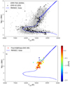 |
Fig. 1. a: HR Diagram of iDR5 FGK stars (grey points), K2 C3 stars analysed in Gaia-ESO iDR5 (black stars) and PARSEC Solar track. b: Kiel diagram of the final set of K2@Gaia-ESO stars for which we obtained spectroscopic parameters as analysed in this paper, with PARSEC Solar track. |
2.2. Preliminary spectroscopic parameters
It was important to initiate the iterations between the spectroscopic and seismic analyses from the best starting point possible in Teff. As not all of the K2@Gaia-ESO targets were observed in time to be included in iDR5, it was necessary to compile the rest of the preliminary stellar parameter set from a variety of other sources including: a photometric Teff; parameters associated with the synthetic template used in the radial velocity determination in the reduction pipelines; and parameters derived using an available Gaia-ESO node analysis. These values are provided for just the 90 K2@Gaia-ESO stars with asteroseismic detections in Table C.1 along with the Gaia-ESO CNAME, EPIC identifier and the instrument with which the spectrum was observed for Gaia-ESO.
For both samples, the infrared flux method (IRFM) calibrations of Ramírez & Meléndez (2005) were used to estimate a photometric Teff using the APASS V magnitude and the 2MASS Ks magnitude. The [Fe/H] from the iDR5 recommended parameters were used as input to the IRFM calibration equations where possible. Otherwise the [Fe/H] from the GIRAFFE radial velocity determination (Gilmore et al., in prep.) were used for GIRAFFE, and the [Fe/H] from the Gaia-ESO Nice Node iDR5 analysis (see Smiljanic et al. 2014; Worley et al. 2016, for description) were used for UVES.
2.3. Outliers
The sample was then investigated for outliers and discrepancies within this range of parameters, which are discussed below.
2.3.1. Signal-to-noise
The signal-to-noise ratio (S/N) is a good indicator of the quality of the observed spectra. The distribution of the S/N for the UVES and GIRAFFE samples for the 90 K2 stars are shown in Fig. 2. The majority of the spectra have S/N above 50. Those spectra with the lowest S/N may potentially suffer from insufficient signal causing deviations in the derived stellar parameters. This is considered in Sect. 3.4 in light of the stellar parameters determined by the two analysis teams.
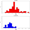 |
Fig. 2. S/N distribution for the K2 stars observed with (a) UVES and (b) GIRAFFE. |
2.3.2. IRFM not applicable
There were three cases for which the magnitudes of the stars did not lie within the range of acceptable values to which the IRFM calibration relations can be applied. They are CNAMEs: 22072768−1440392, 22092416−0610474, and 22105015−1119135. The preliminary parameters were, however, complete for each and were thus used without an assessment against an IRFM Teff. Otherwise the median difference between the IRFM and preliminary Teff is 20 ± 75 K, showing good agreement in general.
2.3.3. No iDR5 [Fe/H]
For the target with CNAME 22034179−0815421 and EPIC ID K2_206298620, no recommended [Fe/H] was reported for iDR5, although Teff and log g were provided. The radial velocity determination provided an associated [Fe/H] of −2.55, however the Teff associated with the radial velocity determination was greater than the iDR5 Teff by ∼300 K and the log g was lower by ∼0.3. The IRFM Teff was in better agreement with the iDR5 Teff. An inspection of the spectrum using iSpec (Blanco-Cuaresma et al. 2014) was carried out, based on a comparison with synthetic spectra generated at both the iDR5 parameters and at the radial velocity determination parameters. In both cases, the [Fe/H] was re-derived, obtaining −2.08 and −1.80, respectively. Based on this and the agreement with the IRFM Teff, the preliminary parameter estimate for this star was supplemented by [Fe/H] = −2.08 derived from the iDR5 parameters using iSpec.
Based on the preliminary set being complete in Teff and in reasonable agreement with the available photometric Teff, the preliminary Teff from spectroscopy were used to derive the preliminary log g from seismology using the seismic analysis described in Paper I carried out by the Birmingham team (hereafter referred to as BHAM).
2.4. Initial spectroscopic parameters
The set of preliminary Teff and [Fe/H] compiled in Table C.1 are comprehensive but were unavoidably inconsistent in their source because not all of them were processed previously by the Gaia-ESO Survey. Thus, for the 90 stars found to have asteroseismic detections an initial analysis using just iSpec was carried out solely on these stars. For this analysis, the surface gravity was fixed to the preliminary seismic log g that was based on the preliminary Teff. This now homogeneous set from iSpec was used to explore any further inconsistencies between the iSpec spectroscopic and preliminary seismic results and fill in missing values as in Sect. 2.3. The iSpec spectroscopic, Teff, was used to determine an associated seismic log g. These comprise the initial set of parameters used as the starting point for the following iterative process between the two Gaia-ESO spectroscopic analyses and the seismic analysis. These initial parameters are listed in Table C.1.
3. Iterative determination of parameters
The goal of this process was to iterate between the spectroscopic effective temperature (Teff,Spec) and the seismic surface gravity (log gSeis) to converge on a final set of independently-confirmed stellar parameters. The seismic log g was determined considering the parameters determined from seismology, namely the frequency of maximum power (νmax) from the p-mode pulsation analysis and the spectroscopic parameter, Teff. We follow the scaling relation of:
 (1)
(1)
as in Morel & Miglio (2012). Details of how this analysis works can be further found in Morel et al. (2014) for a sample of CoRoT targets and in Pinsonneault et al. (2018) for stars observed with Kepler and APOGEE. As discussed there, the seismic analysis of the p-modes is model-independent and so, the main source of uncertainty stems from the input temperature. Therefore, as the Teff,Spec determination improves, the log gSeis determination also improves.
We point to the discussion of Morel et al. (2014) that a change of 100 K in Teff only affects log g by about 0.005. Therefore, significant improvement in log g by, say, a change of the order of 0.1, requires a change in Teff that is much larger than typical uncertainties of Teff. Nonetheless, by fixing log g to a value that is primarily only affected by νmax allows us to set a spectroscopic Teff scale that is consistent with the seismic log(g) and leads to improvement in other stellar quantities such as chemical composition, masses and ultimately ages (see also discussion in Paper I).
Two Gaia-ESO analysis nodes, EPINARBO and Lumba (see Smiljanic et al. 2014, for further details of these and other nodes), carried out the spectroscopic analysis of the GIRAFFE and UVES spectra of the K2 stars in the iterative procedure. The analysis methods are based on equivalent widths for EPINARBO and spectrum synthesis for Lumba (see Sects. 3.2 and 3.3). Following the requirements of the Gaia-ESO Survey, both methods use MARCS stellar atmosphere models (Gustafsson et al. 2008) and the Gaia-ESO linelist (Heiter et al. 2020). These two nodes were selected because they represent two of the most widely used methods for parameter determination in stellar spectroscopy (equivalent widths and syntheses, see Jofré et al. 2019). Figure 3 illustrates the iterative process between spectroscopic and seismic parameter determinations that was followed in this analysis.
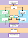 |
Fig. 3. Flow diagram of iterations between spectroscopic and seismic parameter determination. |
In summary, the initial spectroscopic parameters (Teff, iniSpec, [Fe/H]iniSpec) were used to determine the initial seismic log giniSeis. This set of Teff, iniSpec, [Fe/H]iniSpec and log giniSeis were given to both spectroscopic nodes. EPINARBO and Lumba were asked to fix the log g of their analysis to log giniSeis and could otherwise use Teff, iniSpec and [Fe/H]iniSpec as priors in the re-determination of those values if needed.
EPINARBO and Lumba each then returned a new set of parameters, Teff, Spec1 and [Fe/H]Spec1. Based on the Teff, Spec1 values, BHAM then calculated new log gSeis1 values for each node. With their respective sets of log gSeis1 values EPINARBO and Lumba once again determined the parameters based on the fixed log gSeis1 to each provide Teff, Spec2 and [Fe/H]Spec2.
The two sets of Teff, Spec2 and [Fe/H]Spec2 were then combined to define the final set of spectroscopic parameters Teff, finSpec and [Fe/H]finSpec. Based on Teff, finSpec BHAM calculated the final seismic log gfinSeis.
These three values: Teff, finSpec, [Fe/H]finSpec, and log gfinSeis comprise the final stellar parameters of the K2@Gaia-ESO sample. In the final phase EPINARBO and Lumba were then asked to derive chemical abundances for each star based on these stellar parameters.
This was the defined procedure and goal of the K2@Gaia-ESO special project. However the homogenisation and combination of the results into a single final set of parameters per star required a detailed investigation of individual results. This was to ensure that each result was well-understood in an informed manner, which allows for reproducibility. We note that a careful homogenisation of the different node results has been a crucial focus of the Gaia-ESO Survey (Hourihane et al., in prep.; Worley et al., in prep.).
3.1. Homogenisation strategy
There were six sets of Teff, six sets of [Fe/H] and four sets of log g produced in the iterative process. Within these sets are the high-resolution (UVES: 62 targets) and medium-resolution (GIRAFFE: 28 targets) subsamples. The high- and medium-resolution results were homogenised separately, as the lower resolution and smaller wavelength range of the GIRAFFE observations required more detailed quality assessment. The individual node results and the analysis undertaken to homogenise them are explained in the subsequent sections.
3.2. EPINARBO analysis
The EPINARBO analysis measures the equivalent widths (EW) with the DOOp code (Cantat-Gaudin et al. 2014), which automatically measures equivalent widths with DAOSPEC (Stetson & Pancino 2008). It then derives the stellar parameters and abundances with FAMA (Magrini et al. 2014), which calls spectrum synthesis code MOOG (Sneden et al. 2012). The initial microturbulence parameter (ξ) was computed with the Gaia-ESO relation for stars with different Teff and log g (Smiljanic et al. 2014).
For the K2@Gaia-ESO analysis, the surface gravity was fixed to the provided seismic value and EPINARBO iterated to converge on the equilibrium Teff, [Fe/H] and ξ. The stars for which the analysis found a lack of sufficient Fe I and Fe II lines were flagged by EPINARBO and, in particular, it was noted that the blended lines in the medium-resolution GIRAFFE spectra were not ideal for EW methods.
Figure 4 shows the progression of the EPINARBO results iteration. Figures 4a–c compare the initial parameters (Teff, iniSpec, log giniSeis, [Fe/H]iniSpec) to each iterated set of parameters (red: Teff, Spec1, log gSeis1, [Fe/H]Spec1; blue: Teff, Spec2, log gSeis2, [Fe/H]Spec2) for the UVES analysis. Figures 4d–f are the same but for GIRAFFE.
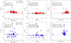 |
Fig. 4. Stellar parameter iterations for EPINARBO (a–c) UVES sample; (d–f) GIRAFFE sample. For Teff, log g and [Fe/H], comparison of initial parameters against Spec1 and Spec2. The median of differences and MAD values are specified. |
The median and median absolute difference (MAD) of the difference between iteration sets for each parameter and each iteration are also shown. There is little variation from Spec1 to Spec2 for both UVES and GIRAFFE. GIRAFFE shows more scatter in the results while the UVES results seem more stable. The plots of seismic log g are included for completeness showing that any large variation in Teff between iterations does not result in much variation in the log g. This agrees with the findings of Morel et al. (2014). See Sect. 3.4 for more discussion on this.
3.3. Lumba analysis
The Lumba analysis (Gavel et al. 2020) performs spectrum synthesis using Spectroscopy Made Easy (SME: Valenti & Piskunov 1996; Piskunov & Valenti 2017). For the K2@Gaia-ESO analysis, the surface gravity was fixed to the provided seismic value and Lumba iterated to converge on the equilibrium Teff, [Fe/H], and ξ (Smiljanic et al. 2014).
Figure 5 shows the iterative process for the Lumba UVES and GIRAFFE analyses as for Fig. 4. There are some distinct outliers for each instrument set, however, the Lumba results are generally very stable between iterations as expected (Morel et al. 2014).
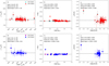 |
Fig. 5. Stellar parameter iterations for Lumba (a–c) UVES sample; (d–f) GIRAFFE sample. For Teff, log g and [Fe/H], comparison of initial parameters against Spec1 and Spec2. The median of differences and MAD values are specified. |
3.4. Comparison of node parameters
Within the Gaia-ESO Survey, all of the nodes perform a fully spectroscopic analysis of the Gaia-ESO spectra. While the determination of unconstrained spectroscopic Teff, log g, and [Fe/H] was not the goal of this study, it is interesting to compare the unconstrained spectroscopic parameters to those determined by iteration between spectroscopy and astereoseismology. For the purposes of this paper, the unconstrained spectroscopic Teff, log g, and [Fe/H] determined by each node are referred to as Spec0.
Figure 6 directly compares the EPINARBO and Lumba parameters derived for Spec0 (top row) and for the final iteration, Spec2 (bottom row), for GIRAFFE (blue), and UVES (red), respectively. Based on Figs. 4 and 5, there was little movement between iterations for each node. Therefore inspecting the final parameters (Spec2) from each node was deemed sufficient. The median and MAD for each parameter between the two nodes are also given. The greater spread of the difference in the GIRAFFE parameters compared to the UVES parameters is clearly seen. The UVES results are in good agreement between the nodes for both Spec0 and Spec2.
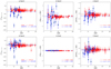 |
Fig. 6. Comparison between the EPINARBO and Lumba parameters against signal-to-noise (S/N) determined for Spec0 in the top row and Spec2 in the bottom row. Left to right: the panels compare spectroscopic Teff, spectrocopic/seismic log g, and spectroscopic [Fe/H], in turn, for UVES (red) and GIRAFFE (blue) spectra. Yellow circles are stars rejected by EPINARBO for inconsistent Fe I and Fe II abundances in Spec0. Central white circles (GIRAFFE) or white triangle (UVES) are stars rejected by EPINARBO for inconsistent Fe I and Fe II abundances in Spec2. The median and MAD of the difference is given for each. |
As stated in Sect. 3.2, EPINARBO reported that the EW method found inconsistencies in Fe I and Fe II abundances for the GIRAFFE spectra due to the blending of spectral features at that resolution and, indeed, a total of nine stars are not included at all for GIRAFFE Spec0 as the EW method did not converge on a result. The particular stars with converged results but that were flagged by EPINARBO are highlighted in all panels in Fig. 6 as data points with a yellow circle as those rejected by EPINARBO in Spec0, and data points with central white dots (GIRAFFE), or white triangles (UVES) as those rejected by EPINARBO in Spec2. The use of the EPINARBO flagged stars for assessing the quality of the results is explained in detail in Sect. 3.4.2.
For Spec0 even those that are not rejected have a wide spread, while for Spec2 the stars that are not rejected are tightly distributed and in good agreement with the Lumba results. Certainly this comparison shows that for the GIRAFFE spectra (lower resolution and smaller wavelength range that UVES) fixing the log g using astereoseismology has allowed the spectroscopic Teff to be better constrained and, thus, there is better agreement between the methods and more of the sample is available for abundance analysis. The high-resolution and greater wavelength range of the UVES sample produces good agreement between the nodes results for both Spec0 and Spec2.
The differences in node parameters in Fig. 6 are shown against S/N. There is no obvious indication that as the S/N decreases, the differences between the node parameters increase. Indeed, for the UVES sample, the spread in the differences is fairly consistent and minimal across the S/N range for both Spec0 and Spec2. For the GIRAFFE sample, there is a large scatter generally for this smaller sample of 28 stars. As there was no obvious trend with S/N, the differences between the node parameters were used directly in the assessment of the quality of the results.
Considering the Spec2 results in particular, which are the set from which the final stellar parameters will be determined, there is, overall, an offset in [Fe/H] between the nodes for both the UVES and GIRAFFE analyses (Δ[Fe/H] ≃ −0.15). There is an offset in Teff (ΔTeff ≃ −80 K). This is discussed further in Sect. 3.4.7.
The log g in all cases are those from the seismic analysis, based on the respective spectroscopic Teff. There are some high discrepancies found between the nodes (ΔTeff > 500 K, Δ[Fe/H] > 0.5) for certain stars, most particularly in the GIRAFFE analysis reflected in the high value of the MAD (MADTeff > 308 K, MAD[Fe/H] > 0.15) compared to the tighter agreement for the UVES analyses (MADTeff > 60 K, MAD[Fe/H] > 0.07). The largest disagreement in Teff equates to a very small shift in seismic log g (ΔTeff ≈ −2200 K corresponds to Δlog g ≈ −0.09).
Figure 7 shows the difference between the two sets of node results for the final seismic log g against the difference in final spectroscopic Teff upon which the final seismic log g values are based. In cyan we show the typical uncertainties for Teff and log g when determined spectroscopically. Differences in spectroscopic Teff greater than 500 K equate to less than a 0.1 difference in seismic log g, which agrees with the discussion in Sect. 3. While asteroseismology pinpoints the log g, it does so from a large potential range in Teff. Therefore, complementary methods are needed, such as spectroscopy, to accurately converge on all stellar parameters.
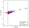 |
Fig. 7. Node difference in final seismic log g against the difference in final Teff for the high (red) and medium (blue) resolution data. Typical spectroscopic uncertainties are shown in cyan. |
The goal at this point was to combine the EPINARBO and Lumba Spec2 results to produce a final spectroscopic Teff (and [Fe/H]) from which a final seismic log g could be calculated. However, prior to this, it was important to understand the differences between the node analyses, particularly with regard to stars for which there was large disagreement, as we did not want to blindly assume that a mean of the parameters from the two nodes was sufficient as a best final value. To assess the goodness of the results, ancillary information was compared to the differences in the parameters to ensure that the results that were selected were of the best quality possible.
Information that was considered was: (1) Node uncertainties on parameters; (2) Quality assessment reported by Nodes; (3) Microturbulence (ξ); (4) Normalised χ2 between observed and synthetic spectra; and (5) Comparison to photometric Teff.
As stated above, there was no obvious trend with S/N so it was not considered in the following quality assessment. The IRFM and Node final parameters are given in Table C.2 for the UVES and GIRAFFE samples.
3.4.1. Uncertainties on parameters
Figure 8 shows the uncertainty distributions for the spectroscopic parameters Teff and [Fe/H] for both EPINARBO and Lumba for the GIRAFFE and UVES analyses. There is a systematic offset between the node distributions and EPINARBO reports a tighter distribution (with strict upper limit for Teff) than Lumba for both the UVES and GIRAFFE samples.
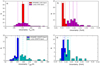 |
Fig. 8. Uncertainty distribution for Teff and [Fe/H] for EPINARBO and Lumba for UVES (a and b), and GIRAFFE (c and d). The median for each distribution is shown as a dashed line with the respective colour, ±σ is shown as dotted lines. |
Each node has reported the uncertainties as best suits their analysis pipelines and, thus, they are internally consistent. However, the uncertainties are not calculated in the same way between the nodes. Due to this difference, they cannot be used to compare the node results (i.e. as a weight) to determine the best value for individual stars.
The difficulty of making comparisons between node results based on the respective uncertainty distributions, when the uncertainties are not defined in a standard way, has been a challenge throughout the lifetime of the Gaia-ESO Survey and for studies in Galactic Archeaology in general. Further discussions on uncertainty analyses can be found in Jofré et al. (2019).
3.4.2. Quality assessment
EPINARBO provided a list of stars for which the sample of Fe I and Fe II lines was inadequate for a robust analysis. These are indicated with a “*” in the CNAME column of Table C.2. There are eight of these stars within the GIRAFFE analysis and 1 star within the UVES analysis.
The uncertainty distribution of the Lumba results shows high tails inferring less confidence in the parameter determination for those stars. Objects with Teff uncertainty > 294 K (244 K; median Teff uncertainty + 3σ) and [Fe/H] uncertainty > 0.28 (0.28; the median [Fe/H] uncertainty + 3σ) were assumed to indicate lower confidence by Lumba in the parameters for the GIRAFFE (UVES) samples.
3.4.3. Microturbulence (ξ)
The ξ was provided by the nodes for both the GIRAFFE and UVES analyses. The ξ relation derived based on iDR1 was used often as a starting point for iterations or as a derived value depending on the respective node procedures. The difference between node ξ values were in some cases very high, particularly for the GIRAFFE analysis.
Figure 9 compares the node ξ values for both the (a) UVES and (b) GIRAFFE analyses directly with a colourmap of ΔTeff, LM − EP. For UVES, there was one star with a large difference in ξ, but otherwise there was no strong evidence of Δξ correlating with ΔTeff. For GIRAFFE the extreme differences in ξ typically were accompanied by other extremes in parameters which are described below. A difference of ξ > 1 km s−1 was used as a threshold when considered alongside the other indicators of goodness of fit.
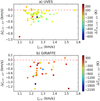 |
Fig. 9. ΔξLM − EP against ξLM with a colourmap of ΔTeff, LM − EP for (a) UVES; (b) GIRAFFE. |
This comparison of the ξ values between the two nodes and the two resolutions for the K2@Gaia-ESO sample revealed an error in the microturbulence relation made available for iDR1. Thanks to this work, the relation was re-derived based on iDR5 values for the iDR6 analysis (see Worley et al., in prep.).
3.4.4. Normalised χ2
It was necessary to independently assess the goodness of fit of the node solutions for the GIRAFFE analyses due to large differences between the reported node parameters. To this end, synthetic spectra for both HR10 and HR21 wavelength ranges were generated for each star using Turbospectrum (Plez 2012) and the MARCS stellar atmosphere models (Gustafsson et al. 2008). Interpolating between the models (Masseron 2006), the spectra were generated at the parameters derived by each node and then a normalised χ2 was calculated between the synthetic spectrum and the observed spectrum. The observed spectrum was normalised to the synthetic spectrum in each case. In this way, the fit was optimised to the solution of each node. The goal was to look for obvious discrepancies in χ2 to discard extreme outliers.
Two measures were used for assessing the goodness indication of the χ2: (a) absolute difference between the EPINARBO χ2 and the Lumba χ2 (|Δχ2|); (b) absolute values of each node χ2.
The set of parameters that represent the best-fit by  between EPINARBO and Lumba was used as the comparison set to avoid assuming that either EPINARBO or Lumba parameters were the best. Figure 10a compares |Δχ2| with
  also showing log|Δχ2| as a colourmap. This log|Δχ2| colourmap is used in Figs. 10b–d to explore the trend with other goodness of fit indicators. When considered in combination with other indicators of goodness of fit, typically all |Δχ2| > 1.0 indicated poor agreement between the nodes and so, in these cases, the node parameter set with the highest χ2 value was rejected. This threshold is shown as a dashed line in Fig. 10a and the rejected points have a white dot at the centre.
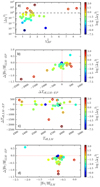 |
Fig. 10. Assessment of rejection criteria based on absolute difference of χ2 between EPINARBO and Lumba. In each case the colourmap is log|Δχ2|: (a) |Δχ2| in a log scale against the best fit (BF) χ2. Rejection limit at 1.0 is shown as a dashed line; (b) Δ[Fe/H]LM − EP against ΔTeffLM − EP; (c) ΔTeff,LM−EP against Teff,LM; (d) Δ[Fe/H]LM − EP against [Fe/H]LM. The data points with a white centre are those rejected when |Δχ2| > 1.0. |
Figure 10b compares the difference in [Fe/H] between the nodes with the difference in Teff between the nodes. Typically, when one is large, the other is large, and the log|Δχ2| is also large, as expected. Figures 10c and d explore whether there is any trend of log|Δχ2| and ΔTeff,LM−EP with Teff,LM−EP, and any trend of log|Δχ2| and Δ[Fe/H]LM − EP with [Fe/H]LM, in case a particular part of the parameter space was particularly susceptible. The Lumba Teff and [Fe/H] were used as reference. There were no obvious trends in either case.
3.4.5. Photometric Teff
The GIRAFFE sample showed, in particular, large disagreements between the two sets of node results. A comparison to the photometric Teff provided another useful indicator as the photometric and spectroscopic Teff should be in relatively good agreement. Interstellar extinction is not expected to play a significant role in the photometric colours as these stars are towards the Galactic pole. When considered in combination with the other indicators, a difference of Teff > 250 K between the photometric and spectroscopic Teff was empirically defined as being too great.
3.4.6. Final GIRAFFE spectroscopic parameters
The final spectroscopic stellar parameters (Teff, [Fe/H], ξ) of the 28 stars in the GIRAFFE sample were defined by first inspecting the node results using the criteria as described above to reject any poor parameter determinations (see Table C.2 for the photometric and node parameters, and the outlier assessment, as well as Table C.3 for the final spectroscopic parameters). In these cases, the remaining node parameter set was used as indicated in Col. 4 of Table C.3. There were 12 cases where only one of the node parameter sets was used. For eight of these cases, EPINARBO had reported large discrepancies between the Fe I and Fe II abundances, or a lack of suitable Fe II lines, for these stars. The χ2 test confirms these as poor fits to the data, with the Lumba node providing significantly better fitting results.
The remaining four cases were considered as follows:
-
CNAME 22082566−1532383: The large discrepancies between the EPINARBO Teff and the IRFM Teff (−288 K), and also the Lumba Teff (−360 K), considered with the large discrepancy between the EPINARBO ξ and the Lumba ξ (−1.29 km s−1) indicated that there were issues with the EPINARBO result and so the Lumba result was taken as the final parameter set.
-
CNAME 22114679−1126477: Similarly, the large discrepancies between the EPINARBO Teff and the IRFM Teff (−455 K), and also the Lumba Teff (−497 K), considered with the large discrepancy between the EPINARBO [Fe/H] and the Lumba [Fe/H] (−0.55) indicated that there were issues with the EPINARBO result and so, the Lumba result was taken as the final parameter set.
-
CNAME 22032304−0754111: The large discrepancy between the EPINARBO χ2 and the Lumba χ2 (−1.81) indicated an issue with the fit to the data; in this case, EPINARBO had the worst fit. This was borne out by inspecting the individual HR10 and HR21 χ2 values, for which the HR21 χ2 values were comparable between the nodes, but the EPINARBO χ2 for HR10 was significantly worse. The difference in Teff reflected this. The Lumba result was taken as the final parameter set.
-
CNAME 22154067−0627110: The discrepancy above the threshold of 1.0 between the EPINARBO χ2 and the Lumba χ2 (−1.06) indicated an issue with the fit to the data; also in this case EPINARBO had the worst fit. Inspection of the individual HR10 and HR21 χ2 values also showed that the HR21 χ2 values were comparable between the nodes, but the EPINARBO χ2 for HR10 was significantly worse. The difference in Teff reflected this. The Lumba result was therefore taken as the final parameter set.
3.4.7. Final UVES spectroscopic parameters
The final spectroscopic stellar parameters (Teff, [Fe/H], ξ) of the 62 stars in the UVES sample were defined also by first inspecting the node results using the criteria as described above to reject any poor parameter determinations. Overall, there was much better agreement between Lumba and EPINARBO for the UVES sample than for the GIRAFFE sample and so, it was not necessary to derive the independent χ2 as an additional measure of goodness of fit. The difference in Teff and [Fe/H] between nodes is seen in Fig. 6. While there is a mean difference that is comparable to the scatter, we are not in a position to favour one node over the other since we do not have reference values for stars of this sample. For Gaia-ESO, both nodes have been independently calibrated with the common set of reference parameters of the Gaia FGK benchmark stars. Therefore, it is not a straightforward task to decide which of the nodes in this particular case, where the pipelines were adapted to iterate with seismology, might be less accurate. In this light, the average of the node results were taken as the final spectroscopic parameters. See Table C.2 for the photometric and node parameters and the outlier assessment, as well as Table C.3 for the final spectroscopic parameters.
There are two remaining cases where the differences are significantly larger and are considered as follows:
-
CNAME 22000793−1203412: The large discrepancies between the Lumba Teff and the IRFM Teff (−263 K) considered with the large discrepancy between the EPINARBO ξ and the Lumba ξ (−0.90 km s−1) and the very large uncertainty on the Lumba Teff (512 K) and [Fe/H] (0.50) indicated that there were issues with the Lumba result and so the EPINARBO result was taken as the final parameter set.
-
CNAME 22032202−0829154: EPINARBO flagged this star as the only UVES star that they found to have a large discrepancy between the abundances derived from the Fe I and Fe II lines. The EPINARBO and Lumba Teff disagree by ΔTeff, LM − EP = −679 K. Both do not agree well with the IRFM Teff with differences of −296 K and 383 K respectively. The initial spectroscopic Teff derived from iSpec was 4643 K, which also does not agree with the IRFM Teff nor EPINARBO. There is, however, no substantial difference between the seismic log g derived for each node (0.03). As EPINARBO flags an issue between the Fe I and Fe II, the Lumba parameters were taken as the final set. In the subsequent chemical analysis, the final Fe I and Fe II are in good agreement (Fe I−Fe II = 0.1), confirming this choice of parameters.
3.5. Final K2@Gaia-ESO stellar parameters
The homogenisation process carried out above resulted in the final catalogue of stellar parameters for the 90 K2@Gaia-ESO red giant stars. These are shown in Fig. 1, with the [Fe/H] as a colourmap. The final stellar parameters are list in Table C.3 and are provided in the final K2@Gaia-ESO catalogue of parameters and abundances which is available at the CDS. The columns of the full catalogue are listed in Table B.1.
4. K2@Gaia-ESO chemical abundances
The final phase of the analysis was the measurement of chemical abundances for those elements typically measured for Gaia-ESO by each node. Based on the final set of stellar parameters (Teff, log g, [Fe/H], and ξ), each node determined their typical chemical abundances for the GIRAFFE and UVES spectra. The nodes provided abundances per star and also abundances per spectral line.
The homogenisation was undertaken using the line-by-line abundances in order for the results to be combined in a more informed way such that the effect of each spectral feature is considered separately. Even with the detailed work required to produce a refined, high-quality line list (Heiter et al. 2020), some of the spectral features used here are less well-modelled than others, which can be due to less robust line information or a strong influence coming from surrounding features, or less robust normalisation of the continuum about that feature. The larger pool of values for each spectral feature across the two nodes compared to a single global value from each node allows for the outlying spectral features to be identified and discarded, if needed, and for features that are in good agreement between the nodes to be more highly weighted.
This was carried out only for those elements for which at least one of the nodes measured more that 50% of the sample, that is, more than 14 stars for GIRAFFE and more than 31 stars for UVES. The threshold of 50% was chosen to meet the requirement for a reference set to be as complete as possible in the reported measurements across all the stars in the set. The node results for any element with less than these thresholds were discarded. The remaining elements and number of K2 stars that were measured by each node and the median number of spectral lines each node measured per element are listed in Table 1.
Elements measured for each element by EPINARBO and Lumba for the GIRAFFE and UVES K2 stars.
The compilation of spectral lines used for Gaia-ESO is described in Heiter et al. (2020) and the individual sources for the spectral lines for each element, summarised in Heiter et al. (2020), are as follows: Na I – Ralchenko et al. (2010); Mg I – Ralchenko et al. (2010); Al I – Wiese et al. (1969); Si I – Garz (1973), Kurucz (2007); Si II – Kurucz (2012); Ca I – Drozdowski et al. (1997), Kurucz (2007), Smith (1981), Smith & O’Neill (1975), Smith (1988), Smith & Raggett (1981); Ca II – Seaton et al. (1994); Sc I – Lawler & Dakin (1989); Sc II – Kurucz (2009), Lawler & Dakin (1989); Ti I – Kurucz (2010), Nitz et al. (1998), Lawler et al. (2013); Ti II – Wood et al. (2013), Kurucz (2010), Ryabchikova et al. (1994); V I – Kurucz (2009); Cr I – Wallace & Hinkle (2009), Kurucz (2010), Sobeck et al. (2007); Cr II – Sigut & Landstreet (1990), Kurucz (2010), Pinnington et al. (1993); Mn I – Kurucz (2007), Den Hartog et al. (2011); Fe I – Kurucz (2007), Fuhr et al. (1988), Bard et al. (1991), O’Brian et al. (1991), Bard & Kock (1994); Fe II – Blackwell et al. (1980), Kurucz (2013); Co I – Kurucz (2008); Ni I – Kurucz (2008), Wickliffe & Lawler (1997); Cu I – Kurucz (2012); Zn I – Lambert et al. (1969), Warner (1968); Y II – Biémont et al. (2011), Kurucz (2011), Pitts & Newsom (1986), Hannaford et al. (1982); Zr I – Biemont et al. (1981); Zr II – Ljung et al. (2006), Cowley & Corliss (1983); Ba II – Miles & Wiese (1969); La II – Lawler et al. (2001a); Ce II – Lawler et al. (2009); Nd II – Meggers et al. (1975), Den Hartog et al. (2003); Eu II – Lawler et al. (2001b).
4.1. Line-by-line cleaning
Lines were accepted or rejected following the rules outlined in Smiljanic et al. (2014), but with appropriate modifications as this project has results from only two nodes, rather than upward of three nodes for the full Gaia-ESO WG11 homogenisation. This meant Rules 1, 2, and 3 of the full Gaia-ESO WG11 homogenisation process were not applicable here. Also, we did not apply the weights based on the parameters used in Smiljanic et al. (2014) so Rule 7 was also not applicable. The remaining rules (4, 5, 6, 8) were applied as follows:
-
Rule 4: When information of the EWs was available, only lines with 5 ≤ EW(mÅ) ≤ 120 were used. Exceptions were sodium (5 ≤ EW(mÅ) ≤ 140) and barium (5 ≤ EW(mÅ) ≤ 250). This could only be applied for the EW node EPINARBO and no cases outside the limits were found for these stars.
-
Rule 5: If, for a given species at a given star, abundances from 20 or more different spectral lines were available, we removed the ones that are flagged as blended in the Gaia-ESO line list (U). This was applied as specified.
-
Rule 6: If […] the total number of spectral lines with abundances (for a given species of a given star) is more than 20, a 2σ clipping from the mean value was applied. (The total number of lines is counted across all nodes, therefore if eight nodes provide abundances for five lines each, it counts as 40 lines for the clipping). This was adapted to the total lines from the two nodes.
-
Rule 8: The median value of multiple lines is adopted as the recommended abundance. This was adapted to be the median of all lines from both nodes.
The reported spectral lines from each node were “cleaned” so to include only those lines flagged as Y or U in the two Gaia-ESO line list flags gf_flag and synflag, except in the case of Rule 4 above. The definition of the Gaia-ESO line list flags are taken from Heiter et al. (2020) and are as follows:
-
gf_flag
-
Y: data which are considered highly accurate, or which were the most accurate ones available for the element under consideration at the time of compilation.
-
U: Data for which the quality is not decided
-
N: Data which are considered to have low accuracy.
-
-
synthflag
-
Y: Line is unblended or only blended with line of same species in both stars (Sun and Arcturus).
-
U: Line may be inappropriate in at least one of the stars.
-
N: Line is strongly blended with line(s) of different species in both stars.
-
The reported abundances are thus the median of the remaining line-by-line abundances once the above rules and cleaning were applied. The associated uncertainty was then the MAD converted to a standard deviation by the scale factor of 1.48 (σ = MAD × 1.48).
In the cases of Cr II and Zr II for UVES, and Ca I, Cr I and Y II for GIRAFFE, only one node provided results for a sufficient number of stars and these were based on one spectral line only. This resulted in an associated uncertainty of zero by the above prescription. In these cases, the uncertainty reported by the node on the spectral line was taken as the uncertainty.
Also, in some cases, the associated uncertainty for a particular star for an element was calculated to be zero while the remaining stars for that element had a non-zero associated uncertainty by the above prescription. In those cases, the median non-zero uncertainty and the MAD converted to sigma on the non-zero uncertainty was calculated from the rest of the sample. A lower threshold was set as the median non-zero uncertainty minus twice the sigma. All associated uncertainties lower than this were set instead to this threshold.
4.2. Intra-node corrections
There were seven elements (Mg I, Al I, Si I, Ca I, Ti II, Ni I, Y II), for which combining the results proved difficult due to systematic offsets between the GIRAFFE and UVES datasets of each node. The seven sets of per instrument and per node results are shown in Fig. A.1.
As there were no stars in common between the GIRAFFE and UVES datasets the way to assess an offset was to look at the overlapping region in [Fe/H] [−0.8 to −0.4] between the two datasets per node. Two assumptions were made to assess the magnitude and direction of the corrections: (1) results from a single node should be continuous in [Fe/H] between the UVES and GIRAFFE results; (2) the Node abundance values around solar metallicity should be similar to the solar abundance.
These allowed the assessment of an offset (difference of the medians across the [Fe/H] range) and the direction of the correction. For instance, for Mg I the EPINARBO GIRAFFE and UVES medians disagree by 0.3 in the overlapping [Fe/H] region. However, we expect solar Mg I at solar [Fe/H], hence the correction was applied to the EPINARBO UVES results. This assessment was carried out resulting in the offsets in Table 2 which were then applied at the per-line level.
Node systematic offsets calculated between GIRAFFE and UVES medians across the [Fe/H] range for seven elements and the node-instrument dataset to which they were applied.
4.3. Comparison of chemical species
Seven of the elements considered here have measurements for both the neutral and ionised species: Ca, Cr, Fe, Sc, Si, Ti, and Zr. A comparison between species is shown in Figs. 11 and 12. GIRAFFE values (blue points) were only available for Ti and Fe.
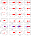 |
Fig. 11. Comparing neutral and ionised species of Ca, Cr, Sc, Si, Ti, and Zr as [X I/Fe] against [X II/Fe], and X I−X II against [Fe/H], Teff, and log g. Median and MAD of the difference between species of the same element are shown. Red displays the UVES sample, blue displays the GIRAFFE sample. |
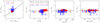 |
Fig. 12. Comparing neutral and ionised species of Fe as [Fe I/Fe] against [Fe II/Fe], and Fe I−Fe II against [Fe/H], Teff, and log g. Median and MAD of the difference between species of the same element are shown. Red displays the UVES sample, blue displays the GIRAFFE sample. Stars flagged by EPINARBO in the parameter round as having inconsistent Fe I and Fe II are indicated as white dots for GIRAFFE and a yellow triangle for UVES. |
In most cases, there is an offset between species on the order of the scatter on the difference. For Zr, for which the median offset is 0.31 ± 0.11, the largest uncertainties correspond to the stars with the greatest disagreement. Typically for all elements the individual stars with largest difference have a large uncertainty on one of the species measurements. There are no obvious trends with any of the parameters.
Figure 12 compares Fe I with Fe II, then the difference of these against [Fe/H], Teff and log g. These are the abundances derived for each species of Fe using the final set of stellar parameters. They are distinct from, but based on, the stellar parameter [Fe/H] which is the global metallicity determined in the parameter round. There is excellent agreement between Fe I and [Fe/H] for both the UVES (−0.03 ± 0.02) and GIRAFFE (0.03 ± 0.05) samples. The agreement for Fe II is less good, showing a larger offset with [Fe/H] for UVES (−0.11 ± 0.04), as well as a large offset and much larger scatter for GIRAFFE (0.13 ± 0.14).
In particular, for GIRAFFE, 10 of the 28 stars have a Fe I−Fe II > 0.2, which is the median combined error on the abundance differences of the species for the GIRAFFE spectra. Two of these have a difference greater than 0.5.
At the parameter determination stage, EPINARBO flagged stars for which the Fe I and Fe II abundances were inconsistent. These are indicated with white dots for GIRAFFE and as a yellow triangle for the single UVES spectrum in Fig. 12. While some of these are still outliers, some have been reclaimed as now being consistent between Fe I and Fe II.
Of the two with Fe I and Fe II abundance differences greater than 0.5, only CNAME 22063424−1530038 was flagged by EPINARBO in the parameter round as having inconsistent Fe I and Fe II abundances. There was also a difference in Spec2 Teff between the nodes of 504 K. Consequently only the Lumba parameters were used for the final parameters (see Table C.3). This star has an outlying rotational velocity which is discussed further in Sect. 6.2.
CNAME 22071427−1431390, also with Fe I−Fe II > 0.5, was not flagged as an outlier during the parameter stage, although there is a difference in the Spec2 [Fe/H] values between Lumba and EPINARBO of −0.24. It has, however, been flagged as a potential binary (see Sect. 6). Two other spectra with Fe I−Fe II > 0.5 were also flagged as potential binaries: CNAMEs 22003290−0808595, 22031541−0753433.
To further understand the possible source of inconsistencies for the remaining seven GIRAFFE stars, for GIRAFFE, the Fe II value is based on a maximum of two spectral lines and only comes from the EPINARBO analysis, compared to at least nine lines for the Fe I value from both EPINARBO and Lumba (see Table 1). Additionally, the Fe II lines are also typically weaker and thus more difficult to measure in medium- compared to high-resolution spectra, resulting in less certain values as indicated by the larger uncertainty bars.
For UVES, 3 of the 62 stars have a Fe I−Fe II > 0.16, which is the median combined error on the abundance differences of the species for the UVES spectra, although none of these have a difference greater than 0.3. None of these three (CNAMEs 22065112−1504580, 22195215−1234594, 22021848−1139147) were identified as an outlier in the parameter homogenisation. CNAME 22065112−1504580 has the largest difference between Fe I and Fe II of −0.28 and it is the only one of these three to be flagged as a potential binary (see Sect. 6).
We note that the ionisation equilibrium (consistent abundance values between neutral and ionised species) may not have been achieved in these cases because the log g value was constrained by non-spectroscopic data, which may reflect shortcomings of the atmospheric models used in the spectroscopic analysis, such as the LTE and 1D prescriptions.
4.4. K2@Gaia-ESO final chemical abundances
The final chemical abundances for the K2@Gaia-ESO stars with the above corrections applied are shown in full in Fig. C.1. The full catalogue table is available at the CDS but the columns are provided in Table B.1. The UVES (high-resolution) and GIRAFFE (medium-resolution) measurements are shown separately. In general the two resolutions track each other for each element distribution, with the improvements due to the corrections applied above. Overall, there appears to be greater scatter in the GIRAFFE datasets, which is not unexpected, particularly for those elements where the measured spectral lines are weak or more blended at lower resolutions (see figures in e.g. Jofré et al. 2019).
The final stage of this work is focussed on the derivation of ages and masses within the greater K2 Galactic Caps Project (see Paper I). Specifically for this paper, the ages of the K2@Gaia-ESO sample were derived, shown as a colour map on the chemical distribution of key elements in Fig. 13.
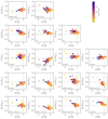 |
Fig. 13. Chemical abundances of [X/Fe] against [Fe/H] for the K2@Gaia-ESO stars with a colourmap of Age. [Fe/H] = 0 and [X/Fe] = 0 are indicated as dashed lines. |
This set of elements is arranged in five key nucleosynthetic channels: Light odd-Z, α, Fe-Peak, s-process and r-process. Each of these channels reflect different nucleosynthetic origins in stellar evolution. Elements created in the same channel show similar behaviour in chemical distribution morphology. These are interpreted in consideration of the recent release of the GALAH DR2 abundances presented in Buder et al. (2019) which used a pipeline which was developed based on the experience with the Lumba pipelines. We note that this is a qualitative comparison only. On the one hand, there are no stars in common between this sample and GALAH DR2. In fact, Gaia-ESO and GALAH only have a small overlap in observed targets (the Gaia benchmark stars, some targets in M67 and the CoRoT fields). On the other hand, our methodology differs from the standard Gaia-ESO parameters so direct comparison between surveys is not the aim here.
Considering the two Light odd-Z elements, Na I shows the expected trend of depleted Na at low metallicity increasing to ∼0.15 at super-solar metallicity. Its distribution is similar to Ni I and Cu I as expected from previous studies (Buder et al. 2019). On the other hand, Al I shows enhanced Al at low metallicity, although no non-LTE corrections have been applied contrary to Buder et al. (2019). Al behaves similarly to Mg and the other α elements, also noted in Buder et al. (2019). The α elements presented here (Mg I, Ca I, Ti I1) all bear the same morphology of showing enhancement at low metallicity decreasing to solar at solar metallicity, which is the typical chemical distribution of α elements (Buder et al. 2019).
The Fe-peak elements (V I, Mn I, Co I, Ni I, Cu I) show at least four types of morphology. V I is unique in that it stays generally constant with a large scatter over the presented metallicity range, which is consistent with other studies. Mn I also is consistent with other studies showing a clear trend of increasing Mn I with metallicity. Co I, Ni I and Cu I can be grouped with similar if not the same morphology of slightly increasing at the metal-poor end, then slightly decreasing then slightly increasing again at solar. This is also not dissimilar to Na I as noted above. The overall increasing trend with metallicity follows that presented in other studies (Buder et al. 2019) although the behaviour around solar begs further investigation.
The s-process is separated into the light (Y II and Zr II) and Heavy (Ba II, La II, Nd II) s-process peaks. Y II shows a large scatter with there being enhancements and depletions for both old and young stars. This was similarly found in Buder et al. (2019). There are fewer measurements for Zr II, particularly at the metal-poor end, but a similarly large spread is indicated.
For the heavy s-process, there are only few measurements at the metal-poor end but these mostly indicate enhanced levels for metal-poor stars for Ba II, La II and Na II. Despite showing a larger scatter for Ba II, all are fairly constant around solar. Finally, the single r-process element, Eu II, shows enhancements at low metallicity, decreasing to a constant solar values at solar and super-solar metallicities, not unlike the α distributions. Although the sample is small compared to other samples where spectroscopy and seismology is available (e.g. Pinsonneault et al. 2018), even for this sample of 90 stars, the morphology of the different nucleosynthetic channels can be seen.
The key outliers in this sample are the two most metal-poor stars which appear to be quite young (∼2 Gyr). This is discussed further in Sect. 6.
5. K2@Gaia-ESO@Gaia: Parallaxes
The iterative determination of the seismic log g and spectroscopic Teff and [Fe/H] was completed prior to the release of Gaia DR2 in April 2018. However, the parallaxes from Gaia DR2 provide a useful check on the robustness of the final K2@Gaia-ESO surface gravities.
The log g based on the Gaia parallax was calculated using the following additional inputs: the final K2@Gaia-ESO Teff and [Fe/H]; the reddening, E(B − V), assigned to each target as part of the Gaia-ESO dataset was taken from Schlegel et al. (1998); and the 2MASS K band photometry (Skrutskie et al. 2006). Of the 90 stars, only 58 are compared here due to the Gaia parallax either not being available or not good enough (parallax uncertainty was greater than 15%).
An iterative procedure using isochrones to determine the optimal stellar mass and surface gravity based on the Gaia parallaxes was carried out (log giso). Further details on the calculation are provided in Appendix D. For comparison, the surface gravity based on the Gaia parallax assuming only solar mass was also calculated (log gM⊙).
Figure 14a compares log gM⊙ with the final K2@Gaia-ESO log g and Fig. 14b compares log giso with the final K2@Gaia-ESO log g. The mean offset for each are Δlog gM⊙−K2 − 0.20 ± 0.14 and Δlog giso−K2 − 0.08 ± 0.08 respectively. Overall log giso are in better agreement with the K2@Gaia-ESO log g than log gM⊙. The typical reported log g uncertainties of K2 are 0.02 and for the Gaia analysis are 0.13. Spectroscopic log g typical uncertainties are 0.10 to 0.25 for the Gaia-ESO high-resolution UVES spectra (Smiljanic et al. 2014) and 0.15 to 0.40 for the Gaia-ESO medium-resolution GIRAFFE spectra (Worley et al., in prep.).
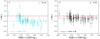 |
Fig. 14. Comparison of log g determined using Gaia parallax with the final K2@Gaia-ESO seismic log g. Cyan points are derived from an initial mass equal to solar, black points are derived from masses based on isochrones. The dashed red line shows the zero difference and the dotted black and cyan lines shows the mean of the differences respectively. |
It is known that the parallaxes provided by Gaia DR2 are affected by systematics (Lindegren et al. 2018; Zinn et al. 2019). A comparison of Gaia parallaxes and K2 seismic parallaxes for stars in the C3 field in Khan et al. (2019) found an offset ranging between −45 and −55 μas. The authors found that the correction in the parallax between Gaia and seismic values seems to depend, to varying degrees, on the position on the sky, the magnitude, and, potentially, the colour. Also, specifically for the K2, C3 and C6 fields, the correction seems to be smaller than in the Kepler field. Following the recommendation in Khan et al. (2019), no ad hoc correction was attempted here but the possible systematics are noted as follows.
Using the equations in Appendix D, the possible range in offsets in parallax corresponds to a range in offsets in log gGaia−K2 of −0.05 to −0.07. This is in the same direction and of similar magnitude to that measured here, showing the offset between parallaxes from Gaia DR2 and asteroseismology found in this study is in agreement with the previous studies (Zinn et al. 2019; Khan et al. 2019).
The main outlier is CNAME 22235003−1422417 with Δlog gGaia−K2 = −0.30 ± 0.16. This star was observed with UVES and had not been flagged as particularly peculiar otherwise. The seismic log g values for each node were in good agreement which is not unexpected as shown above. The difference between the node Teff values is LM-EP = −130 K and [Fe/H] values is LM-EP = −0.39. These are within the acceptable limits imposed in this study for classifying outliers. Three other stars have |Δlog gGaia−K2| > 0.20.
6. K2@Gaia-ESO@Gaia: binary stars
Both the spectra of Gaia-ESO and the astrometric measurements of Gaia offer important information about a star’s movement. These can be combined to study potential binary stars in the sample. This information is given in Table C.4.
We compared the radial velocities (RV) of Gaia-ESO with those from Gaia (Sartoretti et al. 2018; Katz et al. 2019) from the Gaia Radial Velocity Spectrometer (RVS: Cropper et al. 2018). We generally find a very good agreement, with a zero point offset of −0.44 km s−1 for UVES and of −0.95 km s−1 for GIRAFFE, based on which we infer that Gaia-ESO provides systematically lower velocities. The offset is determined from the mean of the RV differences between Gaia and Gaia-ESO. We note the relatively large offset for the GIRAFFE case is based on very few measurements. Indeed, the faint magnitudes of the GIRAFFE sample make the overlap with Gaia RVS very small.
Individual comparisons are shown in Fig. 15, in which we plot the difference of the reported velocities from Gaia-ESO and Gaia as a function of the Gaia uncertainty for all stars that are contained in both datasets. While the majority of the stars have uncertainties in Gaia that are below 1 km s−1, there are a few stars that are more uncertain. There is, however, no relation between Gaia RV uncertainty and apparent magnitude. The values used for the figure can be found in Table C.4.
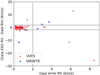 |
Fig. 15. Comparison of radial velocities of Gaia-DR2 and Gaia-ESO as a function of the uncertainty reported by Gaia. Stars that have larger uncertainties than the vertical line at 2 km s−1, or a larger RV difference than the horizontal lines at 2 km s−1, are classified as binaries in this work. |
In addition, by taking a conservative cut of (1) an uncertainty reported by Gaia larger than 1.8 km s−1 or (2) a difference in radial velocities between Gaia and Gaia-ESO larger than 1.8 km s−1, we can select potential binaries. In Fig. 15, lines marking an uncertainty or difference of 1.8 km s−1 are shown vertically and horizontally. It is clear that some stars do not agree that well, falling outside the box marked by the lines within 1.8 km s−1. These measurements might be attributed to binary stars. We note that the reported Gaia RV corresponds to the median of each of various RV measurements at different epochs and its uncertainty may be attributed as the variability in RV for each target. The number of transits varies a lot between each Gaia target, as indicated in Table C.4. A large uncertainty might be related to a large variability, which can be an indication of binary systems (see e.g. recent paper on comparisons of RV of Gaia and RAVE by Birko et al. 2019).
We selected our binaries as those with differences in RV of at least 1.8 km s−1 to account for the intrinsic variation in RV due to jitter, time-variable winds, spot visibility, and so forth, which can have a notable effect in evolved giant stars (see e.g. Carney et al. 2003, for a reference about jitter on metal-poor giants), and for differences of zero point between Gaia-ESO and Gaia, which in our case is for both datasets below 1 km s−1. This gives a total of 14 potential binaries in our sample, corresponding to 15%. This value agrees with the estimate of 17% for metal-poor giants found by Carney et al. (2003) but the comparison should be taken as a reference only since both samples are selected entirely differently. Indeed, the fact that we have been able to provide parameters for the stars implies that no peculiarity in the spectra has been found. It is important to remark that this comparison is also not fully representative as Gaia-DR2 delivered RVs only for stars that are not double-lined spectroscopic binaries. Gaia-ESO, on the other hand, determines RVs for every star, regardless of their binary status. Indeed, a special working group within Gaia-ESO (WG14) analyses double-line spectroscopic binaries and peculiar stars, flagging every target prior to the spectral analysis (Merle et al. 2017, 2020). None of the stars in this sample have been flagged as a double-line spectroscopic binary or as a peculiar star by WG14.
It is worth commenting here that we aimed to identify and investigate the potential binaries that this sample might contain. Yet, variable RV is not the only indication that the star may be a binary. If stars have relatively small RV variation and are binaries at the same time, the companion is likely to be less massive and, so, it exhibits larger RV excursions. As a result, the lines from the companion fall in the wings of the lines of the primary star so that the spectrum appears to be that of a fast rotator, even though in reality it is a set of blended lines. This is seen also in RAVE where the spectrum of a cool dwarf appeared to be a fast rotator, but was ultimately found to be a binary. A similar effect might exist for giants.
In Fig. 16, we plot the ages and metallicities of the stars, coloured according to the respective instrument and indicating in grey the stars that are binaries according to our classification. In general, the expected age-metallicity relation is found, in which metal-poor stars are old and metal-rich stars, can have a wide range of ages. We note that the oldest stars in our sample show ages older than the Universe. As discussed in Paper I, this reflects that the prior used for the age determination was set to a maximum of 20 Gyr. When uncertainties of the results are taken into account, the oldest stars in our sample have ages within the age of the Universe. Here we plot the absolute values with the intention to study their distribution but full details can be found in Paper I.
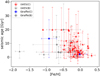 |
Fig. 16. Age-metallicity relation of the stars in our sample. Grey indicates the stars that are binaries (B) and coloured symbols indicate stars that are constant (C) according to our classification (see text). Error bars in age represent the mean between upper and lower age uncertainty estimate (see Paper I). |
We see that two metal-poor stars show notably young ages. For one of them, we have further RV information from Gaia and we note that this star is classified as a possible binary. This star, along with other binary candidates that stand out, are discussed further below.
6.1. EPIC 206101493: potentially an evolved blue straggler
As in several other recent works, some metal-poor (and alpha-enhanced) stars show unexpectedly young ages. The case of EPIC 206101493 is one example found in this K2@Gaia-ESO sample. Its CNAME is 22000793−1203412 and has been observed with UVES.
Such apparently young stars have been reported by Chiappini et al. (2015), and were called “young alpha-rich stars” (YAR). The observation that their high masses might imply they are young (Martig et al. 2015) and their chemical composition is more consistent with that of thick disk stars (Matsuno et al. 2018) challenges our belief that the thick disk formed a long time ago and very rapidly. It is thus very important to first test if they are (or were) binaries, as this determines whether we can or can not apply stellar models of isolated objects to constrain the age of YAR stars. This is discussed in Jofré et al. (2016) with the help of RV monitoring of the YAR stars listed by Martig et al. (2015), and then studied in Izzard et al. (2018) with the help of stellar synthesis models which include the interaction of binary stars. It is thus interesting to see that in our K2@Gaia-ESO sample, EPIC 206101493, as another identified YAR star, is flagged as a binary due to its RV inconsistencies between Gaia-ESO and Gaia.
EPIC 206101493 has a UVES spectrum but since it is one of the faintest stars in our sample, its spectrum has a very low S/N (∼29), this does not allow us to perform a very detailed chemical analysis to investigate its properties further, like Matsuno et al. (2018) did for a sample of these stars. In any case, at a first glance, its parameters are well-determined and its abundances are consistent with a thick disk star. It presents no evident enhancements of s-process or Li. This means that EPIC 206101493 is as typical a thick disk star as the other YAR stars studied in Matsuno et al. (2018), and its high mass agrees with what has been postulated by Jofré et al. (2016), namely, that it is likely a product of mass transfer.
6.2. EPIC 206322094 and EPIC 205977363: induced rotation
In Fig. 17, we show the mass and the projected rotational velocity (v sin i) for our stars, following the same symbols as in previous figures. The projected rotational velocity is determined by Gaia-ESO alongside the radial velocity through the cross-correlation with templates. This is similar to the procedure reported by Carney et al. (2008) for their study of line broadening and rotation of metal-poor giants.
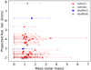 |
Fig. 17. Mass and projected rotational velocity (v sin i) for those stars which have Gaia RV measurements. Error bars in mass represent the mean between upper and lower mass uncertainty estimate (see Paper I). |
We can see that the giants in our sample have typical v sin i of 2−4 km s−1, regardless of their binary status or stellar mass. There are however two stars that stand out, with v sin i > 6 km s−1 (EPIC 206322094 v sin i = 7.85 km s−1; EPIC 205977363 v sin i = 6.25 km s−1). We note there are other stars in our sample with even higher v sin i but they are excluded from this discussion since they do not have RVs from Gaia DR2. While this value is higher than the rest of the stars in the sample, an abundance analysis is still possible and could be done safely.
Giants with these values of rotation have been classified as “anomalous rotators” by Tayar et al. (2015) in the APOKASC sample. They are attributed to be the cause of a recent interaction. As extensively discussed by Carney et al. (2008), the higher broadening of these stars is not likely to be due to macroturbulence. There is a trend for macroturbulence with stellar parameters which is not followed for the outlier cases. This suggests that something else might be causing the broadening. Carney et al. (2003) offer other interesting explanations for outstanding line broadening which are worthy of note.
EPIC 206322094 (CNAME 22031541−0753433) is marked as a binary, and its line broadening might be reflecting an induced rotation due to tidal interactions. Gaia reports an uncertainty in RV of 2.5 km s−1. If the star is tidally interacting with a companion, then its orbit must be circular, which can be tested with individual RV measurements. Unfortunately, this information is still not available from Gaia, but a follow-up campaign on this star is ongoing and will be reported on in a separate paper.
The other star with outlying rotational velocity is EPIC 205977363 (CNAME 22063424−1530038), however, this star does not show indication of having a binary companion from its radial velocity behavior. The star could be the result of a merger (Tayar et al. 2015). Another interesting possibility for its increase in vrot is the capture of a giant planet of few Jupiter masses due to which the star grew in size and became a red giant. It has been shown in the literature that this process can spin up giants a few km s−1 depending on the planet mass and the stellar radius (Privitera et al. 2016).
Siess & Livio (1999) have studied this scenario extensively, discussing possible effects that can be observed. One effect of planet capture is mass loss, which can be detected by the presence of an emission feature or asymmetry in the Hα line. Alternatively, recent discussion in the literature connects Li-rich giants to planet engulfment, where the Li abundance now unexpectedly present in the star was initially material from the planet (see e.g. discussions in Casey et al. 2016, using Gaia ESO data, and references therein). Although it is not entirely clear that engulfment might explain all Li-rich stars (see e.g. Aguilera-Gómez et al. 2016). Since this star is observed with the GIRAFFE setup, we do not have information about the Li abundance or the Hα profile unless a spectrum covering this wavelength domain is undertaken in the future.
6.3. EPIC 206070270 and its unseen companion
In our sample, we have one star (EPIC 206070270 – CNAME 22182719−1252466) with a notably large uncertainty in RV as determined by Gaia (above 8 km s−1). The radial velocities measured by Gaia-ESO and Gaia differ by 25 km s−1, which is consistent with the large RV uncertainty. While this is probably due to it being a binary system, without single RV measurements it is difficult to know for sure. However it is possible that this star is similar to the binaries identified in APOGEE by Price-Whelan et al. (2018). In their catalogue, they use the RV variation (and single epoch RV visit) of APOGEE giants to find the properties of possible binaries. The spectrum is further used to determine the stellar parameters and hence the mass of the giant. The stellar masses they determined cover a range that encompasses the mass of EPIC 206070270 as determined by seismology. Furthermore, they show examples of giants with high variations in RV, in some cases reaching the 25 km s−1 we find here. This value is also a typical value for giants found by the study of mutiplicity of giants in APOGEE by Badenes et al. (2018). If we consider that this difference is the maximum amplitude of the RV variation, and that the giant has a mass of 1.2 M⊙ (see Paper I), we can use the information in Table 5 of Price-Whelan et al. (2018) to estimate that the companion of EPIC 206070270 must be a star with approximately half a solar mass.
The fact that we can constrain the mass and age of the primary with asteroseismology makes this system a potentially interesting target for follow-up studies of RV to constrain the orbits and masses of the secondary. This campaign is taking place already with the HERMES telescope in La Palma and the results will be presented elsewhere once enough RV measurements and a sufficient time span has been achieved to robustly determine the parameters of the binary system.
7. Discussion and conclusion
This work presents a detailed study to determine the stellar parameters of 90 red giant stars by combining results from spectroscopy and asteroseismology. The spectroscopy comes from data taken as part of the Gaia-ESO Survey in a project designed to expand the available set of calibration samples. The asteroseismology comes from data taken by K2 in the C3 field. The parameters could therefore be determined with higher accuracy due to the iterative procedure of deriving Teff from the spectra to be used as input for deriving log g from oscillation frequencies which is then used to re-derive Teff. A substantial change in Teff results in just a small change in the seismic log g and so both methods are required to ensure the required accuracy in parameters.
Understanding the origin of the Galactic disks is based on a fundamental question and the answer is sought in the exploitation of stellar surveys. However, there are underlying challenges due to the inaccuracy of the stellar parameters and abundances derived for metal-poor and ancient stars. Having as many reference stars as possible in this regime is key to finding the answer.
The C3 field was chosen as it points towards the South Galactic Pole, thus favouring the inclusion of thick disk and metal-poor stars. These stars are under-represented in other seismic fields, notably the Kepler field (see Rendle et al. 2019 for the space distribution of the stars of K2C3 and Kepler). In addition, a study of chemical abundance evolution and binary detection was performed given the additional information pertaining to the masses and ages from K2, as well as the information of Gaia DR2.
The spectroscopic analysis was based on the combination of two distinct methods, both of which are part of the analysis procedure of the Gaia-ESO data. One method was based on spectrum synthesis and the other one was based on equivalent widths. Together, they allowed us to assess systematic uncertainties and reliability of results, thus providing a catalogue of spectral parameters and abundances that is accurate and not biased towards a given methodology. However, based on the intra-node abundance assessment and the corrections that were needed for seven of the elements, some possible systematic offsets in individual element abundances may remain.
The combination of seismology and spectroscopy allows us to analyse trends of abundances as a function of age, finding, as expected, that more metal-poor and α-capture element-enhanced stars are older. The addition of the Gaia DR2 data also allows us to identify possible binary stars: the ones that are suspiciously more massive for their metal-content, those rotating unusually faster, or those having differences in radial velocities that are larger than expected.
Catalogues of parameters and abundances for which both seismology and spectroscopy are available are few. Pioneering works in this direction are the APOKASC sample (Pinsonneault et al. 2014, 2018) and the CoRoGEE sample (Anders et al. 2017). Hawkins et al. (2016) published a catalogue with abundances for this sample considering the infrared APOGEE spectra based on temperatures determined photometrically and surface gravities from scaling relations of Kepler.
Another group at the forefront of this work is led by Valentini et al. (2017), who published a study similar to the one presented here (i.e. iterating between spectroscopy and seismology to reach to consistent parameters). They analysed 87 giants observed by RAVE. The spectra are of intermediate resolution (R ∼ 7000) and cover a short wavelength range around the Ca II triplet, equivalent to Gaia RVS. In Valentini et al. (2017) it is possible to see how the overall stellar parameters improve when seismology is available. The group further performed a follow-up, detailed, high-resolution study of four metal-poor stars of their sample, which is presented in Valentini et al. (2019). The full RAVE catalogue will soon become public (Steinmetz et al. 2020). Targets with seismology have proven to be fundamental for the calibration of surface gravities of RAVE (Kunder et al. 2017). Similarly, Gaia-ESO is in the process of using CoRoT data as part of the calibration plan (Pancino et al. 2017), with the intention to publish the CoRoT@Gaia-ESO catalogue (Masseron et al., in prep.). In Valentini et al. (2016), the UVES and GIRAFFE stars were analysed following the same procedure as for the RAVE study.
Recently, Sharma et al. (2019) presented a study of the age and metallicity gradient of a large sample of K2 stars observed in GALAH. The study includes the same fields we analyse here, but GALAH spectra are currently not public to the entire community. The parameters and abundances are part of GALAH DR2 (Buder et al. 2018), although they were not derived using the seismic parameters as a prior.
In addition, Nissen et al. (2017) published a catalogue of parameters and abundances derived self consistently with seismology using high-resolution optical spectra of HARPS-N for a sample of solar twins in Kepler. Finally, Morel et al. (2014) presents the study of high resolution optical spectra of 20 red giants that were targeted by CoRoT.
Our work is a novel contribution as the largest high-resolution optical catalogue with parameters and abundances derived homogeneously. We have taken advantage of forefront spectroscopic and astereoseismic methodologies, along with the sample targets of the outer regions of the disk to capture sought-after old and metal-poor stars. Our catalogue of parameters and abundances is available at the CDS, including the results at a line-by-line and method-by-method level to ensure reproducibility (see Tables B.1 and B.2 for list of columns). The spectra are public via the ESO archives. In addition, the chosen field of K2 was selected so that our catalogue would include more thick disk stars than other samples for which spectroscopy and astereoseismology are available.
While the interior of stars gives us clues as to their evolutionary phase (based on mass and age), the exterior of stars tell us about their formation site (chemistry), and stellar motion (radial velocities). Individually, these latter two types of data can provide the means to calibrate the analysis of large samples of stars, however, the combination of both provides an even more powerful basis upon which to make a more effective and robust analysis that is key to constraining models of galactic formation and evolution.
Ti behaves observationally like the rest of the α elements.
Acknowledgments
The authors thank the International Space Science Institute in Bern (ISSI) and Beijing (ISSI-BJ) for supporting and hosting the meetings of the International Team on “AsteroStep” and “Libraries of 2020”, respectively, during which the discussions leading and contributing to this publication were initiated and held. PJ acknowledges support of FONDECYT Iniciación Grant Number 11170174. RS acknowledges support from the National Science Centre (2014/15/B/ST9/03981). A.G., A.K. and U.H. acknowledge support from the Swedish National Space Agency (SNSA/Rymdstyrelsen). T.B. was funded by the project grant “The New Milky Way” from the Knut and Alice Wallenberg Foundation. This work is based on data products from observations made with ESO Telescopes at the La Silla Paranal Observatory under programme ID 188.B-3002. These data products have been processed by the Cambridge Astronomy Survey Unit (CASU) at the Institute of Astronomy, University of Cambridge, and by the FLAMES/UVES reduction team at INAF/Osservatorio Astrofisico di Arcetri. These data have been obtained from the Gaia-ESO Survey Data Archive, prepared and hosted by the Wide Field Astronomy Unit, Institute for Astronomy, University of Edinburgh, which is funded by the UK Science and Technology Facilities Council. This work was partly supported by the European Union FP7 programme through ERC grant number 320360 and by the Leverhulme Trust through grant RPG-2012-541. We acknowledge the support from INAF and Ministero dell’ Istruzione, dell’ Università’ e della Ricerca (MIUR) in the form of the grant “Premiale VLT 2012”. The results presented here benefit from discussions held during the Gaia-ESO workshops and conferences supported by the ESF (European Science Foundation) through the GREAT Research Network Programme. The authors thank the anonymous referee for the useful comments that improved the manuscript.
References
- Aguilera-Gómez, C., Chanamé, J., Pinsonneault, M. H., & Carlberg, J. K. 2016, ApJ, 829, 127 [NASA ADS] [CrossRef] [Google Scholar]
- Anders, F., Chiappini, C., Rodrigues, T. S., et al. 2017, A&A, 597, A30 [NASA ADS] [CrossRef] [EDP Sciences] [Google Scholar]
- Badenes, C., Mazzola, C., Thompson, T. A., et al. 2018, ApJ, 854, 147 [NASA ADS] [CrossRef] [Google Scholar]
- Baglin, A., Auvergne, M., Barge, P., et al. 2006, in The CoRoT Mission Pre-Launch Status – Stellar Seismology and Planet Finding, eds. M. Fridlund, A. Baglin, J. Lochard, & L. Conroy, ESA Spec. Publ., 1306, 33 [Google Scholar]
- Bard, A., & Kock, M. 1994, A&A, 282, 1014 [NASA ADS] [Google Scholar]
- Bard, A., Kock, A., & Kock, M. 1991, A&A, 248, 315 [NASA ADS] [Google Scholar]
- Biemont, E., Grevesse, N., Hannaford, P., & Lowe, R. M. 1981, ApJ, 248, 867 [NASA ADS] [CrossRef] [Google Scholar]
- Biémont, É., Blagoev, K., Engström, L., et al. 2011, MNRAS, 414, 3350 [NASA ADS] [CrossRef] [Google Scholar]
- Birko, D., Zwitter, T., Grebel, E. K., et al. 2019, AJ, 158, 155 [CrossRef] [Google Scholar]
- Blackwell, D. E., Shallis, M. J., & Simmons, G. J. 1980, A&A, 81, 340 [NASA ADS] [Google Scholar]
- Blanco-Cuaresma, S., Soubiran, C., Heiter, U., & Jofré, P. 2014, A&A, 569, A111 [NASA ADS] [CrossRef] [EDP Sciences] [Google Scholar]
- Borucki, W. J., Koch, D., Basri, G., et al. 2010, Science, 327, 977 [NASA ADS] [CrossRef] [PubMed] [Google Scholar]
- Bressan, A., Marigo, P., Girardi, L., et al. 2012, MNRAS, 427, 127 [NASA ADS] [CrossRef] [Google Scholar]
- Buder, S., Asplund, M., Duong, L., et al. 2018, MNRAS, 478, 4513 [NASA ADS] [CrossRef] [Google Scholar]
- Buder, S., Lind, K., Ness, M. K., et al. 2019, A&A, 624, A19 [NASA ADS] [CrossRef] [EDP Sciences] [Google Scholar]
- Cantat-Gaudin, T., Donati, P., Pancino, E., et al. 2014, A&A, 562, A10 [NASA ADS] [CrossRef] [EDP Sciences] [Google Scholar]
- Carney, B. W., Latham, D. W., Stefanik, R. P., Laird, J. B., & Morse, J. A. 2003, AJ, 125, 293 [NASA ADS] [CrossRef] [Google Scholar]
- Carney, B. W., Latham, D. W., Stefanik, R. P., & Laird, J. B. 2008, AJ, 135, 196 [NASA ADS] [CrossRef] [Google Scholar]
- Carpenter, J. M. 2001, AJ, 121, 2851 [NASA ADS] [CrossRef] [Google Scholar]
- Casey, A. R., Ruchti, G., Masseron, T., et al. 2016, MNRAS, 461, 3336 [NASA ADS] [CrossRef] [Google Scholar]
- Chiappini, C., Anders, F., Rodrigues, T. S., et al. 2015, A&A, 576, L12 [NASA ADS] [CrossRef] [EDP Sciences] [Google Scholar]
- Cirasuolo, M., & MOONS Consortium 2016, in Multi-Object Spectroscopy in the Next Decade: Big Questions, Large Surveys, and Wide Fields, eds. I. Skillen, M. Balcells, & S. Trager, ASP Conf. Ser., 507, 109 [Google Scholar]
- Cowley, C. R., & Corliss, C. H. 1983, MNRAS, 203, 651 [NASA ADS] [CrossRef] [Google Scholar]
- Cropper, M., Katz, D., Sartoretti, P., et al. 2018, A&A, 616, A5 [NASA ADS] [CrossRef] [EDP Sciences] [Google Scholar]
- Dalton, G., Trager, S. C., Abrams, D. C., et al. 2012, in Ground-based and Airborne Instrumentation for Astronomy IV, Proc. SPIE, 8446, 84460P [CrossRef] [Google Scholar]
- de Jong, R. S., Agertz, O., Berbel, A. A., et al. 2019, The Messenger, 175, 3 [NASA ADS] [Google Scholar]
- Den Hartog, E. A., Lawler, J. E., Sneden, C., & Cowan, J. J. 2003, ApJS, 148, 543 [Google Scholar]
- Den Hartog, E. A., Lawler, J. E., Sobeck, J. S., Sneden, C., & Cowan, J. J. 2011, ApJS, 194, 35 [NASA ADS] [CrossRef] [Google Scholar]
- De Silva, G. M., Freeman, K. C., Bland-Hawthorn, J., et al. 2015, MNRAS, 449, 2604 [NASA ADS] [CrossRef] [MathSciNet] [Google Scholar]
- Drozdowski, R., Ignaciuk, M., Kwela, J., & Heldt, J. 1997, Z. Phys. D At. Mol. Clust., 41, 125 [CrossRef] [Google Scholar]
- Elias, J. H., Frogel, J. A., Matthews, K., & Neugebauer, G. 1982, AJ, 87, 1029 [NASA ADS] [CrossRef] [Google Scholar]
- Fuhr, J. R., Martin, G. A., & Wiese, W. L. 1988, Journal of Physical and Chemical Reference Data (New York: American Institute of Physics (AIP) and American Chemical Society), 17 [Google Scholar]
- Gaia Collaboration (Brown, A. G. A., et al.) 2018, A&A, 616, A1 [NASA ADS] [CrossRef] [EDP Sciences] [Google Scholar]
- Garz, T. 1973, A&A, 26, 471 [NASA ADS] [Google Scholar]
- Gavel, A., Gruyters, P., Korn, A., Lind, K., & Nordlander, T. 2020, A&A, 629, A74 [Google Scholar]
- Gilmore, G., Randich, S., Asplund, M., et al. 2012, The Messenger, 147, 25 [NASA ADS] [Google Scholar]
- Gustafsson, B., Edvardsson, B., Eriksson, K., et al. 2008, A&A, 486, 951 [NASA ADS] [CrossRef] [EDP Sciences] [Google Scholar]
- Hannaford, P., Lowe, R. M., Grevesse, N., Biemont, E., & Whaling, W. 1982, ApJ, 261, 736 [NASA ADS] [CrossRef] [Google Scholar]
- Hawkins, K., Masseron, T., Jofré, P., et al. 2016, A&A, 594, A43 [NASA ADS] [CrossRef] [EDP Sciences] [Google Scholar]
- Heiter, U., Jofré, P., Gustafsson, B., et al. 2015, A&A, 582, A49 [NASA ADS] [CrossRef] [EDP Sciences] [PubMed] [Google Scholar]
- Heiter, U., Lind, K., Bergemann, M., et al. 2020, A&A, submitted [Google Scholar]
- Houdashelt, M. L., Bell, R. A., & Sweigart, A. V. 2000, AJ, 119, 1448 [Google Scholar]
- Howell, S. B., Sobeck, C., Haas, M., et al. 2014, PASP, 126, 398 [NASA ADS] [CrossRef] [Google Scholar]
- Izzard, R. G., Preece, H., Jofre, P., et al. 2018, MNRAS, 473, 2984 [NASA ADS] [CrossRef] [Google Scholar]
- Jofré, P., Heiter, U., Soubiran, C., et al. 2014, A&A, 564, A133 [NASA ADS] [CrossRef] [EDP Sciences] [Google Scholar]
- Jofré, P., Jorissen, A., Van Eck, S., et al. 2016, A&A, 595, A60 [NASA ADS] [CrossRef] [EDP Sciences] [Google Scholar]
- Jofré, P., Heiter, U., Tucci Maia, M., et al. 2018, Res. Notes Am. Astron. Soc., 2, 152 [NASA ADS] [CrossRef] [Google Scholar]
- Jofré, P., Heiter, U., & Soubiran, C. 2019, ARA&A, 57, 571 [Google Scholar]
- Katz, D., Sartoretti, P., Cropper, M., et al. 2019, A&A, 622, A205 [NASA ADS] [CrossRef] [EDP Sciences] [Google Scholar]
- Khan, S., Miglio, A., Mosser, B., et al. 2019, The Gaia Universe, 13 [Google Scholar]
- Kunder, A., Kordopatis, G., Steinmetz, M., et al. 2017, AJ, 153, 75 [NASA ADS] [CrossRef] [Google Scholar]
- Kurucz, R. L. 2007, Robert L. Kurucz On-line Database of Observed and Predicted Atomic Transitions [Google Scholar]
- Kurucz, R. L. 2008, Robert L. Kurucz On-line Database of Observed and Predicted Atomic Transitions [Google Scholar]
- Kurucz, R. L. 2009, Robert L. Kurucz On-line Database of Observed and Predicted Atomic Transitions [Google Scholar]
- Kurucz, R. L. 2010, Robert L. Kurucz On-line Database of Observed and Predicted Atomic Transitions [Google Scholar]
- Kurucz, R. L. 2011, Robert L. Kurucz On-line Database of Observed and Predicted Atomic Transitions [Google Scholar]
- Kurucz, R. L. 2012, Robert L. Kurucz On-line Database of Observed and Predicted Atomic Transitions [Google Scholar]
- Kurucz, R. L. 2013, Robert L. Kurucz On-line Database of Observed and Predicted Atomic Transitions [Google Scholar]
- Lambert, D. L., Mallia, E. A., & Warner, B. 1969, MNRAS, 142, 71 [NASA ADS] [CrossRef] [Google Scholar]
- Lawler, J. E., & Dakin, J. T. 1989, J. Opt. Soc. Am. B Opt. Phys., 6, 1457 [NASA ADS] [CrossRef] [Google Scholar]
- Lawler, J. E., Bonvallet, G., & Sneden, C. 2001a, ApJ, 556, 452 [NASA ADS] [CrossRef] [Google Scholar]
- Lawler, J. E., Wickliffe, M. E., den Hartog, E. A., & Sneden, C. 2001b, ApJ, 563, 1075 [CrossRef] [Google Scholar]
- Lawler, J. E., Sneden, C., Cowan, J. J., Ivans, I. I., & Den Hartog, E. A. 2009, ApJS, 182, 51 [NASA ADS] [CrossRef] [Google Scholar]
- Lawler, J. E., Guzman, A., Wood, M. P., Sneden, C., & Cowan, J. J. 2013, ApJS, 205, 11 [NASA ADS] [CrossRef] [Google Scholar]
- Lindegren, L., Hernández, J., Bombrun, A., et al. 2018, A&A, 616, A2 [NASA ADS] [CrossRef] [EDP Sciences] [Google Scholar]
- Ljung, G., Nilsson, H., Asplund, M., & Johansson, S. 2006, A&A, 456, 1181 [NASA ADS] [CrossRef] [EDP Sciences] [Google Scholar]
- Magrini, L., Randich, S., Friel, E., et al. 2014, FAMA: Fast Automatic MOOG Analysis [Google Scholar]
- Majewski, S. R., Schiavon, R. P., Frinchaboy, P. M., et al. 2017, AJ, 154, 94 [NASA ADS] [CrossRef] [Google Scholar]
- Martig, M., Rix, H.-W., Silva Aguirre, V., et al. 2015, MNRAS, 451, 2230 [NASA ADS] [CrossRef] [Google Scholar]
- Masseron, T. 2006, PhD Thesis, Observatoire de Paris, France [Google Scholar]
- Matsuno, T., Yong, D., Aoki, W., & Ishigaki, M. N. 2018, ApJ, 860, 49 [CrossRef] [Google Scholar]
- McCall, M. L. 2004, AJ, 128, 2144 [NASA ADS] [CrossRef] [Google Scholar]
- Meggers, W. F., Corliss, C. H., & Scribner, B. F. 1975, Tables of Spectral-line Intensities. Part I, II_- Arranged by Elements, 145 [Google Scholar]
- Merle, T., Van Eck, S., Jorissen, A., et al. 2017, A&A, 608, A95 [NASA ADS] [CrossRef] [EDP Sciences] [Google Scholar]
- Merle, T., Van der Swaelmen, M., Van Eck, S., et al. 2020, A&A, 635, A155 [Google Scholar]
- Miglio, A., Chiappini, C., Mosser, B., et al. 2017, Astron. Nachr., 338, 644 [NASA ADS] [CrossRef] [Google Scholar]
- Miles, B. M., & Wiese, W. L. 1969, At. Data, 1, 1 [Google Scholar]
- Mints, A., & Hekker, S. 2017, A&A, 604, A108 [NASA ADS] [CrossRef] [EDP Sciences] [Google Scholar]
- Morel, T., & Miglio, A. 2012, MNRAS, 419, L34 [NASA ADS] [CrossRef] [Google Scholar]
- Morel, T., Miglio, A., Lagarde, N., et al. 2014, A&A, 564, A119 [NASA ADS] [CrossRef] [EDP Sciences] [Google Scholar]
- Nissen, P. E., Silva Aguirre, V., Christensen-Dalsgaard, J., et al. 2017, A&A, 608, A112 [NASA ADS] [CrossRef] [EDP Sciences] [Google Scholar]
- Nitz, D. E., Wickliffe, M. E., & Lawler, J. E. 1998, ApJS, 117, 313 [NASA ADS] [CrossRef] [Google Scholar]
- O’Brian, T. R., Wickliffe, M. E., Lawler, J. E., Whaling, W., & Brault, J. W. 1991, J. Opt. Soc. Am. B Opt. Phys., 8, 1185 [NASA ADS] [CrossRef] [Google Scholar]
- Pancino, E., Lardo, C., Altavilla, G., et al. 2017, A&A, 598, A5 [NASA ADS] [CrossRef] [EDP Sciences] [Google Scholar]
- Pinnington, E. H., Ji, Q., Guo, B., et al. 1993, Can. J. Phys., 71, 470 [NASA ADS] [CrossRef] [Google Scholar]
- Pinsonneault, M. H., Elsworth, Y., Epstein, C., et al. 2014, ApJS, 215, 19 [NASA ADS] [CrossRef] [Google Scholar]
- Pinsonneault, M. H., Elsworth, Y. P., Tayar, J., et al. 2018, ApJS, 239, 32 [Google Scholar]
- Piskunov, N., & Valenti, J. A. 2017, A&A, 597, A16 [NASA ADS] [CrossRef] [EDP Sciences] [Google Scholar]
- Pitts, R. E., & Newsom, G. H. 1986, J. Quant. Spectr. Radiat. Transf., 35, 383 [NASA ADS] [CrossRef] [Google Scholar]
- Plez, B. 2012, Astrophysics Source Code Library [record ascl:1205.004] [Google Scholar]
- Price-Whelan, A. M., Hogg, D. W., Rix, H.-W., et al. 2018, AJ, 156, 18 [NASA ADS] [CrossRef] [Google Scholar]
- Privitera, G., Meynet, G., Eggenberger, P., et al. 2016, A&A, 593, A128 [NASA ADS] [CrossRef] [EDP Sciences] [Google Scholar]
- Prugniel, P., & Soubiran, C. 2001, A&A, 369, 1048 [NASA ADS] [CrossRef] [EDP Sciences] [Google Scholar]
- Ralchenko, Y., Kramida, A., Reader, J., & NIST ASD Team 2010, NIST Atomic Spectra Database (ver. 4.0.0) [Online] [Google Scholar]
- Ramírez, I., & Meléndez, J. 2005, ApJ, 626, 465 [Google Scholar]
- Rendle, B. M., Miglio, A., Chiappini, C., et al. 2019, MNRAS, 490, 4465 [CrossRef] [Google Scholar]
- Ryabchikova, T. A., Hill, G. M., Landstreet, J. D., Piskunov, N., & Sigut, T. A. A. 1994, MNRAS, 267, 697 [NASA ADS] [CrossRef] [EDP Sciences] [Google Scholar]
- Sartoretti, P., Katz, D., Cropper, M., et al. 2018, A&A, 616, A6 [NASA ADS] [CrossRef] [EDP Sciences] [Google Scholar]
- Schlegel, D. J., Finkbeiner, D. P., & Davis, M. 1998, ApJ, 500, 525 [NASA ADS] [CrossRef] [Google Scholar]
- Seaton, M. J., Yan, Y., Mihalas, D., & Pradhan, A. K. 1994, MNRAS, 266, 805 [NASA ADS] [CrossRef] [Google Scholar]
- Sharma, S., Stello, D., Bland-Hawthorn, J., et al. 2019, MNRAS, 490, 5335 [CrossRef] [Google Scholar]
- Siess, L., & Livio, M. 1999, MNRAS, 308, 1133 [NASA ADS] [CrossRef] [Google Scholar]
- Sigut, T. A. A., & Landstreet, J. D. 1990, MNRAS, 247, 611 [NASA ADS] [Google Scholar]
- Skrutskie, M. F., Cutri, R. M., Stiening, R., et al. 2006, AJ, 131, 1163 [NASA ADS] [CrossRef] [Google Scholar]
- Smiljanic, R., Korn, A. J., Bergemann, M., et al. 2014, A&A, 570, A122 [NASA ADS] [CrossRef] [EDP Sciences] [Google Scholar]
- Smith, G. 1981, A&A, 103, 351 [NASA ADS] [Google Scholar]
- Smith, G. 1988, J. Phys. B At. Mol. Phys., 21, 2827 [NASA ADS] [CrossRef] [Google Scholar]
- Smith, G., & O’Neill, J. A. 1975, A&A, 38, 1 [NASA ADS] [Google Scholar]
- Smith, G., & Raggett, D. S. J. 1981, J. Phys. B At. Mol. Phys., 14, 4015 [NASA ADS] [CrossRef] [Google Scholar]
- Sneden, C., Bean, J., Ivans, I., Lucatello, S., & Sobeck, J. 2012, Astrophysics Source Code Library [record ascl:1202.009] [Google Scholar]
- Sobeck, J. S., Lawler, J. E., & Sneden, C. 2007, ApJ, 667, 1267 [NASA ADS] [CrossRef] [Google Scholar]
- Soubiran, C., Le Campion, J.-F., Brouillet, N., & Chemin, L. 2016, A&A, 591, A118 [NASA ADS] [CrossRef] [EDP Sciences] [Google Scholar]
- Steinmetz, M., Matijevic, G., Enke, H., et al. 2020, AJ, 160, 82 [CrossRef] [Google Scholar]
- Stetson, P. B., & Pancino, E. 2008, PASP, 120, 1332 [Google Scholar]
- Szeto, K., Simons, D., Bauman, S., et al. 2018, in Society of Photo-Optical Instrumentation Engineers (SPIE) Conference Series, Proc. SPIE, 10700, 107001N [Google Scholar]
- Tayar, J., Ceillier, T., García-Hernández, D. A., et al. 2015, ApJ, 807, 82 [NASA ADS] [CrossRef] [Google Scholar]
- Valenti, J. A., & Piskunov, N. 1996, A&AS, 118, 595 [NASA ADS] [CrossRef] [EDP Sciences] [Google Scholar]
- Valentini, M., Chiappini, C., Miglio, A., et al. 2016, Astron. Nachr., 337, 970 [NASA ADS] [CrossRef] [Google Scholar]
- Valentini, M., Chiappini, C., Davies, G. R., et al. 2017, A&A, 600, A66 [NASA ADS] [CrossRef] [EDP Sciences] [Google Scholar]
- Valentini, M., Chiappini, C., Bossini, D., et al. 2019, A&A, 627, A173 [CrossRef] [EDP Sciences] [Google Scholar]
- Wallace, L., & Hinkle, K. 2009, ApJ, 700, 720 [NASA ADS] [CrossRef] [Google Scholar]
- Warner, B. 1968, MNRAS, 140, 53 [NASA ADS] [Google Scholar]
- Wickliffe, M. E., & Lawler, J. E. 1997, ApJS, 110, 163 [CrossRef] [Google Scholar]
- Wiese, W. L., Smith, M. W., & Miles, B. M. 1969, Atomic Transition Probabilities. Vol. 2: Sodium Through Calcium. A Critical Data Compilation (US Government Printing Office) [Google Scholar]
- Wood, M. P., Lawler, J. E., Sneden, C., & Cowan, J. J. 2013, ApJS, 208, 27 [NASA ADS] [CrossRef] [Google Scholar]
- Worley, C. C., de Laverny, P., Recio-Blanco, A., Hill, V., & Bijaoui, A. 2016, A&A, 591, A81 [NASA ADS] [CrossRef] [EDP Sciences] [Google Scholar]
- Zinn, J. C., Pinsonneault, M. H., Huber, D., & Stello, D. 2019, ApJ, 878, 136 [NASA ADS] [CrossRef] [Google Scholar]
Appendix A: Intra-node chemical species corrections
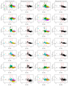 |
Fig. A.1. Chemical abundances of [X/Fe] against [Fe/H] for Mg I, Al I, Si I, Ca I, Ti II, Ni I, and Y II for the K2@Gaia-ESO stars derived based on the final stellar parameters. First column: node (EP,LM) and instrument (U, G) results as specified in the legend. The [Fe/H] overlap is bounded by dashed red lines. The errorbars are the line-by-line values per star per node uncertainties. Second column: homogenised abundances without per node corrections. Third column: node values with corrections applied. Fourth column: final homogenised values. |
Appendix B: K2@Gaia-ESO catalogue columns
Columns contained in the K2@Gaia-ESO Catalogue.
Columns for line-by-line per node per CNAME abundance analysis.
Appendix C: K2@Gaia-ESO chemical abundance distributions
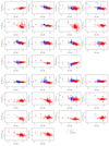 |
Fig. C.1. Chemical abundances of [X/Fe] against [Fe/H] for the K2@Gaia-ESO stars derived based on the final stellar parameters. The UVES stars are red triangles, the GIRAFFE stars are blue circles. [Fe/H] = 0 and [X/Fe] = 0 are indicated as dashed lines. |
90 stars analysed in the K2 Gaia-ESO special project.
Parameters determined by IRFM, the final parameters from each node, the outlier assessment from uncertainties, and the final parameters for the 62 UVES and 28 GIRAFFE stars.
Final stellar parameters for the 90 K2@Gaia-ESO stars.
Radial (RV) and rotational velocities (v sin i) of the K2@Gaia-ESO stars measured by Gaia-ESO and from the Gaia Data Release 2 (GDR2).
Appendix D: Gaia surface gravity
Bolometric corrections were interpolated from the tables of Houdashelt et al. (2000). These corrections are tabulated for the K magnitude in the CIT/CTIO system (Elias et al. 1982). Thus, first the Ks magnitude of 2MASS were converted to KCIT/CTIO using the relations provided by Carpenter (2001).
The bolometric corrections (BC) are mostly independent of log g. First the two tables of metallicity values closest to the metallicity of the star (usually [Fe/H] = 0.00 and [Fe/H] = −0.50) are found. These tables are used to linearly interpolate the corrections to the Teff of the star. Then a second linear interpolation is carried out to the metallicity of the star.
The E(B − V) is converted to AKs using the coefficients of McCall (2004). In this case, AKs/E(B − V) = 0.350.
The absolute magnitude (Mabs) is then:
 (D.1)
(D.1)
where +0.024 is the conversion to KCIT/CTIO and the parallax (π) has to be in arcsec (hence the 0.001)
This implicitly assumes that distance = 1/parallax which is only then calculated if the relative uncertainty of the parallax is better than 15%.
Then the bolometric magnitude (Mbol) and luminosity of the star relative to the Sun log(L*/L⊙) are:
 (D.2)
(D.2)
 (D.3)
(D.3)
where 4.75 is the bolometric magnitude of the Sun.
And finally:
 (D.4)
(D.4)
The stellar masses were then estimated using the UniDAM code2 (Mints & Hekker 2017). It interpolates masses from PARSEC isochrones (Bressan et al. 2012) using a Bayesian scheme. A first estimate of mass was computed with this code using the spectroscopic parameters (Teff, log g, [Fe/H]), 2MASS magnitudes, parallaxes, and extinction.
With this first mass estimate, we compute a first estimate of log g using Eq. (D.4). The new log g values are then given again to UniDAM, to recompute the mass estimates. These iterations were repeated (a total of four iterations was sufficient) until the estimated mass was consistent with the estimated log g.
UniDAM gives an estimate of the error of the mass, and this was also used in the computation of the total error budget in log g. Uncertainties are from 10 000 Monte Carlo simulations, assuming Gaussian uncertainties in π, K2MASS, stellar mass (with error coming from UniDAM), and ±0.02 mag for the bolometric correction. No uncertainty was assumed in E(B − V), nor for Teff⊙, or log g⊙.
All Tables
Elements measured for each element by EPINARBO and Lumba for the GIRAFFE and UVES K2 stars.
Node systematic offsets calculated between GIRAFFE and UVES medians across the [Fe/H] range for seven elements and the node-instrument dataset to which they were applied.
Parameters determined by IRFM, the final parameters from each node, the outlier assessment from uncertainties, and the final parameters for the 62 UVES and 28 GIRAFFE stars.
Radial (RV) and rotational velocities (v sin i) of the K2@Gaia-ESO stars measured by Gaia-ESO and from the Gaia Data Release 2 (GDR2).
All Figures
|
Fig. 1. a: HR Diagram of iDR5 FGK stars (grey points), K2 C3 stars analysed in Gaia-ESO iDR5 (black stars) and PARSEC Solar track. b: Kiel diagram of the final set of K2@Gaia-ESO stars for which we obtained spectroscopic parameters as analysed in this paper, with PARSEC Solar track. |
| In the text | |
|
Fig. 2. S/N distribution for the K2 stars observed with (a) UVES and (b) GIRAFFE. |
| In the text | |
|
Fig. 3. Flow diagram of iterations between spectroscopic and seismic parameter determination. |
| In the text | |
|
Fig. 4. Stellar parameter iterations for EPINARBO (a–c) UVES sample; (d–f) GIRAFFE sample. For Teff, log g and [Fe/H], comparison of initial parameters against Spec1 and Spec2. The median of differences and MAD values are specified. |
| In the text | |
|
Fig. 5. Stellar parameter iterations for Lumba (a–c) UVES sample; (d–f) GIRAFFE sample. For Teff, log g and [Fe/H], comparison of initial parameters against Spec1 and Spec2. The median of differences and MAD values are specified. |
| In the text | |
|
Fig. 6. Comparison between the EPINARBO and Lumba parameters against signal-to-noise (S/N) determined for Spec0 in the top row and Spec2 in the bottom row. Left to right: the panels compare spectroscopic Teff, spectrocopic/seismic log g, and spectroscopic [Fe/H], in turn, for UVES (red) and GIRAFFE (blue) spectra. Yellow circles are stars rejected by EPINARBO for inconsistent Fe I and Fe II abundances in Spec0. Central white circles (GIRAFFE) or white triangle (UVES) are stars rejected by EPINARBO for inconsistent Fe I and Fe II abundances in Spec2. The median and MAD of the difference is given for each. |
| In the text | |
|
Fig. 7. Node difference in final seismic log g against the difference in final Teff for the high (red) and medium (blue) resolution data. Typical spectroscopic uncertainties are shown in cyan. |
| In the text | |
|
Fig. 8. Uncertainty distribution for Teff and [Fe/H] for EPINARBO and Lumba for UVES (a and b), and GIRAFFE (c and d). The median for each distribution is shown as a dashed line with the respective colour, ±σ is shown as dotted lines. |
| In the text | |
|
Fig. 9. ΔξLM − EP against ξLM with a colourmap of ΔTeff, LM − EP for (a) UVES; (b) GIRAFFE. |
| In the text | |
|
Fig. 10. Assessment of rejection criteria based on absolute difference of χ2 between EPINARBO and Lumba. In each case the colourmap is log|Δχ2|: (a) |Δχ2| in a log scale against the best fit (BF) χ2. Rejection limit at 1.0 is shown as a dashed line; (b) Δ[Fe/H]LM − EP against ΔTeffLM − EP; (c) ΔTeff,LM−EP against Teff,LM; (d) Δ[Fe/H]LM − EP against [Fe/H]LM. The data points with a white centre are those rejected when |Δχ2| > 1.0. |
| In the text | |
|
Fig. 11. Comparing neutral and ionised species of Ca, Cr, Sc, Si, Ti, and Zr as [X I/Fe] against [X II/Fe], and X I−X II against [Fe/H], Teff, and log g. Median and MAD of the difference between species of the same element are shown. Red displays the UVES sample, blue displays the GIRAFFE sample. |
| In the text | |
|
Fig. 12. Comparing neutral and ionised species of Fe as [Fe I/Fe] against [Fe II/Fe], and Fe I−Fe II against [Fe/H], Teff, and log g. Median and MAD of the difference between species of the same element are shown. Red displays the UVES sample, blue displays the GIRAFFE sample. Stars flagged by EPINARBO in the parameter round as having inconsistent Fe I and Fe II are indicated as white dots for GIRAFFE and a yellow triangle for UVES. |
| In the text | |
|
Fig. 13. Chemical abundances of [X/Fe] against [Fe/H] for the K2@Gaia-ESO stars with a colourmap of Age. [Fe/H] = 0 and [X/Fe] = 0 are indicated as dashed lines. |
| In the text | |
|
Fig. 14. Comparison of log g determined using Gaia parallax with the final K2@Gaia-ESO seismic log g. Cyan points are derived from an initial mass equal to solar, black points are derived from masses based on isochrones. The dashed red line shows the zero difference and the dotted black and cyan lines shows the mean of the differences respectively. |
| In the text | |
|
Fig. 15. Comparison of radial velocities of Gaia-DR2 and Gaia-ESO as a function of the uncertainty reported by Gaia. Stars that have larger uncertainties than the vertical line at 2 km s−1, or a larger RV difference than the horizontal lines at 2 km s−1, are classified as binaries in this work. |
| In the text | |
|
Fig. 16. Age-metallicity relation of the stars in our sample. Grey indicates the stars that are binaries (B) and coloured symbols indicate stars that are constant (C) according to our classification (see text). Error bars in age represent the mean between upper and lower age uncertainty estimate (see Paper I). |
| In the text | |
|
Fig. 17. Mass and projected rotational velocity (v sin i) for those stars which have Gaia RV measurements. Error bars in mass represent the mean between upper and lower mass uncertainty estimate (see Paper I). |
| In the text | |
|
Fig. A.1. Chemical abundances of [X/Fe] against [Fe/H] for Mg I, Al I, Si I, Ca I, Ti II, Ni I, and Y II for the K2@Gaia-ESO stars derived based on the final stellar parameters. First column: node (EP,LM) and instrument (U, G) results as specified in the legend. The [Fe/H] overlap is bounded by dashed red lines. The errorbars are the line-by-line values per star per node uncertainties. Second column: homogenised abundances without per node corrections. Third column: node values with corrections applied. Fourth column: final homogenised values. |
| In the text | |
|
Fig. C.1. Chemical abundances of [X/Fe] against [Fe/H] for the K2@Gaia-ESO stars derived based on the final stellar parameters. The UVES stars are red triangles, the GIRAFFE stars are blue circles. [Fe/H] = 0 and [X/Fe] = 0 are indicated as dashed lines. |
| In the text | |
Current usage metrics show cumulative count of Article Views (full-text article views including HTML views, PDF and ePub downloads, according to the available data) and Abstracts Views on Vision4Press platform.
Data correspond to usage on the plateform after 2015. The current usage metrics is available 48-96 hours after online publication and is updated daily on week days.
Initial download of the metrics may take a while.