| Issue |
A&A
Volume 642, October 2020
|
|
|---|---|---|
| Article Number | A214 | |
| Number of page(s) | 20 | |
| Section | Interstellar and circumstellar matter | |
| DOI | https://doi.org/10.1051/0004-6361/202039073 | |
| Published online | 22 October 2020 | |
Supernova explosions interacting with aspherical circumstellar material: implications for light curves, spectral line profiles, and polarization★
1
Institute of Theoretical Physics, Faculty of Mathematics and Physics, Charles University,
V Holešovičkách 2,
180 00
Praha 8,
Czech Republic
e-mail: This email address is being protected from spambots. You need JavaScript enabled to view it.
2
Department of Theoretical Physics and Astrophysics, Masaryk University,
Kotlářská 2,
611 37
Brno, Czech Republic
Received:
30
July
2020
Accepted:
17
September
2020
Abstract
Some supernova (SN) explosions show evidence for an interaction with a pre-existing nonspherically symmetric circumstellar medium (CSM) in their light curves, spectral line profiles, and polarization signatures. The origin of this aspherical CSM is unknown, but binary interactions have often been implicated. To better understand the connection with binary stars and to aid in the interpretation of observations, we performed two-dimensional axisymmetric hydrodynamic simulations where an expanding spherical SN ejecta initialized with realistic density and velocity profiles collide with various aspherical CSM distributions. We consider CSM in the form of a circumstellar disk, colliding wind shells in binary stars with different orientations and distances from the SN progenitor, and bipolar lobes representing a scaled down version of the Homunculus nebula of η Car. We study how our simulations map onto observables, including approximate light curves, indicative spectral line profiles at late times, and estimates of a polarization signature. We find that the SN–CSM collision layer is composed of normal and oblique shocks, reflected waves, and other hydrodynamical phenomena that lead to acceleration and shear instabilities. As a result, the total shock heating power fluctuates in time, although the emerging light curve might be smooth if the shock interaction region is deeply embedded in the SN envelope. SNe with circumstellar disks or bipolar lobes exhibit late-time spectral line profiles that are symmetric with respect to the rest velocity and relatively high polarization. In contrast, SNe with colliding wind shells naturally lead to line profiles with asymmetric and time-evolving blue and red wings and low polarization. Given the high frequency of binaries among massive stars, the interaction of SN ejecta with a pre-existing colliding wind shell must occur and the observed signatures could be used to characterize the binary companion.
Key words: supernovae: general / circumstellar matter / shock waves / stars: emission-line, Be / polarization
Movies associated to Figs. 3, 4, 6–9 are only available at the https://www.aanda.org
Note to the reader: the links to the movies webpage have been corrected on 3 March 2021.
© ESO 2020
1 Introduction
When an expanding supernova (SN) blast wave collides with a dense pre-existing circumstellar material (CSM), the gas in the collision region is compressed and becomes radiative. Depending on the CSM properties, a substantial fraction of the SN kinetic energy might be converted into radiation. Such SN–CSM interactions can give rise to transients that are more luminous than ordinary SNe, including a subset of recently-recognized superluminous SNe (e.g., Gal-Yam 2012; Smith 2017). We show light curves of a few examples of interacting SNe in Fig. 1. Since the most radiatively efficient collisions occur with CSM located near the progenitor, the interacting SNe reveal the mass-loss history of massive stars shortly before the collapse of the core (e.g., Smith & McCray 2007; Smith 2014; Stritzinger et al. 2012).
The observed properties of the SN–CSM interaction often require an aspherical CSM distribution. The evidence comes from multicomponent line profiles in SN spectra (e.g., Chugai & Danziger 1994; Fransson et al. 2002; Smith et al. 2015; Andrews et al. 2017; Andrews & Smith 2018), (spectro)polarimetry (e.g., Leonard et al. 2000; Wang & Wheeler 2008; Chornock et al. 2010; Patat et al. 2011), or combinations thereof (Bilinski et al. 2018, 2020). Aspherical CSM can lead to observable outcomes that are qualitatively different from a spherically symmetric SN–CSM interaction. If the shock interaction region subtends only a small fraction of the solid angle as seen from the SN, for example when the CSM is in the form of a disk, the SN ejecta can envelop and surround the shock and hide interaction signatures such as narrow emission lines. The SN can then behave as if there is an additional power source embedded deep in the ejecta. This qualitative picture can explain Type IIn-P SNe and similar objects (Mauerhan et al. 2013; Smith 2013a). A similar geometry of spherical explosion colliding with pre-existing equatorially-confined CSM could explain peculiar SNe, such as iPTF14hls (Arcavi et al. 2017; Andrews & Smith 2018) and AT2018cow (Margutti et al. 2019), transients associated with binary interactions and common envelope events (Metzger & Pejcha 2017; Pejcha et al. 2016a,b, 2017; MacLeod et al. 2018; Hubová & Pejcha 2019), classical novae (Li et al. 2017), and eruptions of very massive stars such as η Car (Smith et al. 2018).
Aspherical CSM can have a number of different angular distributions. The commonly assumed configuration is an equatorially-confined disk with a radially decreasing density. This type of profile is a natural result of binary interactions such as mass transfer or common envelope (e.g., Podsiadlowski et al. 1992; Morris & Podsiadlowski 2007; Kashi & Soker 2010; Smith 2011) as well as equatorial mass loss from rapidly spinning stars (e.g., Heger & Langer 1998; Okazaki 2001; Kraus et al. 2007; Krtička et al. 2011; Kurfürst et al. 2014, 2018).
Other CSM distributions of interest are colliding winds within a binary star, where radiatively-cooled material from both winds accumulates in a dense curved surface resembling a bow shock (e.g., Stevens et al. 1992; Gayley et al. 1997). Since most massive stars are found in binaries (e.g., Sana et al. 2012; Moe & Di Stefano 2017), colliding wind shells must be relatively frequent around core-collapse SNe and might be confused with shells originating in pre-SN progenitor eruptions. Indeed, Kochanek (2019) argue that a binary wind collision shell is a better explanation for the observed flash-ionized spectra of SN 2013fs. The bow shock-like structures resulting from wind collision shells are of particular interest to interacting SNe, because the collision with SN ejecta happens gradually and the interaction region moves progressively farther away from the progenitor star. Depending on the wind momenta of the binary components, the wind collision shell can be curved toward the progenitor, which would make the interaction signatures visible, or away from it, which could potentially hide the narrow lines from a large fraction of viewing angles. Furthermore, the wind collision shells in binary stars are corrugated due to hydrodynamical and radiation instabilities (e.g., Vishniac 1994; Kee et al. 2014; Steinberg & Metzger 2018), which are a natural mechanism for forming clumps (Calderón et al. 2016, 2020). The interaction of SN ejecta with clumpy CSM is expected to produce bumps in the light curves, which are seen in some events (Fig. 1). Curved shells of dense material can also form when the binary companion does not have a strong wind, but it photoionizes a small HII region in the wind of the primary (Braun et al. 2012; Kochanek 2019). Bow shock-like structures on larger scales also arise when red supergiant winds are trapped in a dense CSM shell by external ionizing photons (Mackey et al. 2014).
Finally, the terminal SN explosion can collide with CSM that was shaped by preceding eruptions and their collisions. An example of such an event is the hypothetical future SN explosion of η Car, which will sweep through the Homunculus nebula, which in itself might have been shaped by spherical eruption colliding with pre-existing equatorial outflow (Smith et al. 2018). Given the complex CSM pattern in this case, we expect a complicated behavior of multiple shocks and their mutual interactions.
Much of the theoretical work on observational characteristics of interacting SNe has been done in spherical symmetry (e.g., Chevalier 1982; Moriya et al. 2013; Dessart et al. 2015, 2016), but a few authors have explored SN interacting with aspherical CSM. Blondin et al. (1996) studied axisymmetric hydrodynamical simulations of a spherical self-similar driven wave propagating through a smooth angularly-dependent CSM and found that a protrusion develops in the directions where CSM is rarified. van Marle et al. (2010) performed two-dimensional hydrodynamic simulations of a collision of spherical SN ejecta with a spherical shell embedded in a spherical or an angularly-dependent wind. They estimated light curves by assuming optically thin cooling in the shock interaction region. Vlasis et al. (2016) utilized 2D hydrodynamic simulations with multigroup M1 radiation transport to calculate viewing angle-dependent light curves of various combinations of spherical and angularly-dependent SN ejecta and CSM, and a spherical SN colliding with a relic disk. McDowell et al. (2018) performed moving-mesh hydrodynamic calculations of spherical SN interacting with a disk. They estimated light curves by combining numerical shock heating rates with a diffusive model of SN light curves. Kurfürst & Krtička (2019) conducted two-dimensional hydrodynamic simulations of a spherical SN colliding with circumstellar disks of different masses embedded in spherically symmetric stellar winds with a range of mass-loss rates. Most recently, Suzuki et al. (2019) investigated interaction of a spherical SN ejecta with a circumstellar disk with axisymmetric special-relativistic adaptive mesh refinement hydrodynamics with two-temperature treatment of radiation.They calculated bolometric light curves from different viewing angles and estimated photosphere locations.
Here, we perform high-resolution axisymmetric hydro- dynamic-only simulations of a spherical SN interacting with several aspherical CSM geometries. Our goal is to identify observable signatures that would allow us to discern different CSM geometries from basic SN observables. Since many of the aspherical CSM distributions are linked to various aspects of binary star evolution, constraining the CSM geometry can probe the configuration of the binary. In particular, for the first time we study the hydrodynamical interaction of SN ejecta with colliding wind shells of binary stars. Since our goal is to illuminate qualitative differences between various CSM geometries, we do not attempt to provide models specifically matched to individual SN events.
This paper is organized as follows. Section 2 describes the numerical setup of our calculations. Section 3 describes and compares the hydrodynamic evolutions and discusses the shock interactions. In Sect. 4, we provide approximate estimates of observable quantities based on our models (light curves, spectral line profiles, polarization) and compare these results to the observed SNe. In Sect. 5, we summarize our findings.
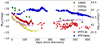 |
Fig. 1 Comparison of light curves of five prominent long-lasting SNe II (after Nyholm et al. 2017). The photometry data are from Aretxaga et al. (1999), Stritzinger et al. (2012), Smith et al. (2009), Nyholm et al. (2017), Arcavi et al. (2017), and were obtained from the Open Supernova Catalog (Guillochon et al. 2017). We convert the r∕R magnitudes to bolometric L according to Eq. (1) in Nyholm et al. (2017), which applies constant zero bolometric correction. |
2 Numerical setup
In this section, we briefly review our numerical code (Sect. 2.1) and describe the initial and boundary conditions for our numerical experiments (Sect. 2.2).
2.1 Description of the code
We conduct the numerical experiments using our Eulerian hydrodynamic code described in detail by Kurfürst et al. (2014, 2018) and Kurfürst & Krtička (2017, 2019). We solve axisymmetric conservative equations of continuity, radial and polar compo- nents of momentum, and total energy on a polar grid described by radial coordinate r and polar coordinate θ. The equations are
![Mathematical equation: \begin{align}&\frac{\partial\rho}{\partial t}+ \frac{1}{r^2}\frac{\partial\widetilde M_r}{\partial r}+ \frac{1}{r\sin\theta} \frac{\partial\widetilde M_{\theta}}{\partial\theta}\,{=}\,0,\\[3pt]&\frac{\partial M_r}{\partial t}+\frac{1}{r^2}\frac{\partial}{\partial r} \left(\widetilde M_r u_{\textrm{r}}\right)+ \frac{1}{r\sin\theta}\frac{\partial}{\partial\theta} (\widetilde M_{\theta} u_{\textrm{r}}) -\rho\frac{u_{\theta}^2}{r}+ \frac{\partial P}{\partial r}\,{=}\,0,\\[3pt]&\frac{\partial M_{\theta}}{\partial t}+\frac{1}{r^2}\frac{\partial}{\partial r} \left(\widetilde M_ru_{\theta}\right)+\! \frac{1}{r\sin\theta}\frac{\partial}{\partial\theta} (\widetilde M_{\theta} u_{\theta}) \!+\!\rho\frac{u_{\textrm{r}} u_{\theta}}{r}\!+\!\frac{1}{r}\frac{\partial P} {\partial\theta}\,{=}\,0,\\[3pt]&\frac{\partial E}{\partial t}+\frac{1}{r^2}\frac{\partial}{\partial r} \left(\widetilde M_r H\right)+ \frac{1}{r\sin\theta}\frac{\partial}{\partial\theta} \left(\widetilde M_{\theta} H\right)\,{=}\,0, \end{align}](/articles/aa/full_html/2020/10/aa39073-20/aa39073-20-eq1.png)
where ρ is the density, ur and uθ are the radial and polar velocity components of the total velocity  , P is the scalar pressure,
  and
and  are the two components of the momentum density, E = ρɛ + ρu2∕2 is the total energy density, ρɛ is the internal energy density, and H = (E + P)∕ρ is the enthalpy. The entire set of hydrodynamic equations is closed by an equation of state of a radiation dominated gas, 3P = ρɛ. We estimate the adiabatic temperaturein the models as
  , where a is the radiation density constant. We estimate the specific entropy of the radiation dominated gas as s = 4aT3∕(3ρ). We perform the calculations in polar coordinates (r, θ), but it is often advantageous to present the results in cylindrical coordinates ϖ = r sinθ and z = r cosθ.
We do not include gravitational forces, because we start our simulations when the fluid velocities are much faster than the local escape velocity, which makes the gravitational forces negligible. Since our focus is primarily on hydrodynamic interactions of the shocks, we do not include explicit viscosity, radioactive heating of the material, nor other effectively internal sources of energy like magnetar spin down. We do not include radiative cooling or any other redistribution of energy due to radiation, which corresponds to an assumption that the interaction region is optically thick and the diffusion time is longer than the expansion time. As the SN expands and the ejecta rarefies, this assumption will be violated. While simulations including radiation exist (Vlasis et al. 2016; Suzuki et al. 2019), proper treatment of radiation is beyond the scope of our work.
2.2 Initial conditions
Our simulations include three components: spherically symmetric SN ejecta (Sect. 2.2.1), spherically symmetric stellar wind surrounding the progenitor star (Sect. 2.2.2), and aspherical CSM. The properties of SN ejecta and spherical wind are the same between different simulations, but we study different types of aspherical CSM: equatorial disk (model A; Sect. 2.2.3), colliding wind shell (models B1, B2a, B2b, and B3; Sect. 2.2.4), and bipolar lobes similar to the Homunculus nebula (model C; Sect. 2.2.5). We describe the construction of the initial conditions of each of our models below in this section.
Our numerical grid covers 0.2 ≤ r∕R⋆ ≤ 450, where R⋆ is the initial radius of SN ejecta, which corresponds to the precollapse radius of the progenitor star. The radial grid is composed of 60 zones covering the initial SN ejecta for 0.2 ≤ r∕R⋆ ≤ 1 and 6000 zones between R⋆ and the outer boundary. The polar grid is uniform across the radial domain with 480 grid cells for simulations covering 0 ≤ θ ≤ π∕2 and 640 cells for simulations covering 0 ≤ θ ≤ 2π∕3. The grid aspect ratio with much denser radial grid than the polar grid contributes to numerical stability by damping the so-called carbuncle instabilities that may develop near shocks (e.g., Pandolfi & D’Ambrosio 2001, see also Kurfürst et al. 2017; Kurfürst & Krtička 2017, 2019).
The boundary conditions at the inner and outer boundaries of the computational domain are free (outflowing). The reflection boundary condition is applied at the symmetry axis. The other lateral boundary is either reflecting or outflowing depending on the nature of the CSM distribution. The values in the grid boundary and ghost zones are extrapolated from the inner mesh computational domain values with a zeroth-order extrapolation. We evolve the system for a physical time of approximately 400–500 d.
Since hydrodynamical instabilities are expected to play a significant role in our setup and we do not regularize our simulations by imposingartificial viscosity, we expect that local details of our results will depend on the numerical resolution. To test that the global properties are not sensitive to the resolution, we performed simulations of model A (Sect. 2.2.3) with half the resolution in radial and polar directions outside of the progenitor. We plot light curves and indicative spectral line profile from this low-resolution run in Figs. 10 and 12, and find very good agreement with the default high-resolution models.
2.2.1 Supernova ejecta
The initial profile of SN ejecta is often approximated with a broken power-law (e.g., Chevalier & Soker 1989; McDowell et al. 2018), but here we use a more realistic initial condition. First, we calculate shock propagation through a realistic progenitor using one-dimensional implicit radiation hydrodynamics code SNEC (Morozova et al. 2015). We use the default progenitor supplied with the code, which is a nonrotating star with the initial mass of 15 M⊙ evolved to the moment of core collapse with the code MESA (Paxton et al. 2011, 2013). Detailed information on the evolution and parameters used in the MESA calculation are given in Sect. 3.2 of Morozova et al. (2015). At the collapse, the progenitor is a red supergiant with the mass of 12.283 M⊙ and radius R⋆ ≈ 7.23 × 1013 cm ≈ 1000 R⊙. We explode the progenitor with a 1051 erg thermal bomb and keep all of the parameters to their default values except for the amount of radioactive nickel, which we set to zero. When the SN shock breaks out of the stellar surface, we remap the density, velocity, temperature, and pressure profiles from SNEC to our code. We show the initial profiles of these quantities in Fig. 2. Rotation of the progenitor star might lead to aspherical SN ejecta, however, to isolate the effect of aspherical CSM, we do focus only on spherical SN ejecta in this work. The effect of aspherical SN ejecta was explored by Vlasis et al. (2016).
2.2.2 Spherical wind
SN ejecta is surrounded by a spherically symmetric wind, which serves primarily as a filling medium to ensure stable numerics. The density and temperature are too low to significantly affect the observed evolution. The density ρwind is set to
 (5)
(5)
where Ṁwind = 10−6 M⊙ yr−1 is the mass-loss rate and thevwind = 15 km s−1 is the asymptotic wind velocity typical for red supergiants (e.g., Goldman et al. 2017). This choice implies the wind base density ρ0,wind ≈ 6.5 × 10⁻¹⁶ g cm−3. Total mass of the spherical wind over the full three-dimensional domain corresponding to our grid is 7 × 10⁻⁴ M⊙. We set the initial stellar wind temperatureprofile to be decreasing as Twind =  , where T⋆ ≈3300 K is the progenitor stellar effective temperature. This corresponds to optically thin wind at radiative equilibrium with the progenitor radiation. At outer regions, the spherical wind has a fixed temperature Twind = 15 K. We set the initial wind pressure and sound speed profile using the solar metallicity ideal gas law and the wind density and temperature. We do not take into account the acceleration of the wind close to the progenitor (Fig. 2). However, this typically affects only the first few days of the SN light curve (Moriya et al. 2018) and we focus our work on later times of the SN evolution.
 |
Fig. 2 Initial profiles of selected hydrodynamic quantities. Black lines show the initial numerical profiles of density ρ, radial velocity ur, pressure P, and temperature T of the SN ejecta (gray region with 0.2 ≤ r∕R⋆ ≤ 1) and of the stellar wind in the close vicinity (r > R⋆). The red lineshows the initial analytical density profile described in Appendix A. |
2.2.3 Model A – equatorial disk
We set the density distribution as a sum of a spherically symmetric wind and an equatorially-concentrated disk. We set the disk density ρdisk following Kurfürst et al. (2018) and Kurfürst & Krtička (2019) as
![Mathematical equation: \begin{align*}\rho_{\text{disk}}\,{=}\,\rho_{0,\text{disk}}\left(\frac{R_{\star}}{r}\right)^{w}\, \exp\left[\frac{2\left(\sin\theta-1\right)}{(H/\mathcal{R})^2}\right], \end{align*}](/articles/aa/full_html/2020/10/aa39073-20/aa39073-20-eq8.png) (6)
(6)
where ρ0,disk ≈ 5 × 10⁻¹⁴ g cm−3 is the mass density at the base of the disk midplane (close to the surface of the SN progenitor star), w = 2 is the power-law index (same as in McDowell et al. 2018), H is the disk vertical scaleheight, and  is the radial distance measured in the disk equatorial plane. We define H = cS∕Ω, where
  is the disk Keplerian angular velocity and cS is set using the same assumptions as for the spherical wind described in Sect. 2.2.3. The total mass of the disk and underlying wind is 5.2 × 10⁻³ M⊙, which is about a factor of ten higher than of the spherical wind alone. The disk parameters were chosen to provide a nontrivial shock interaction that would fit on our numerical grid.
2.2.4 Models B – colliding wind shells
A collision of stellar winds in a binary forms an interface of shocked gas. If the wind collision shocks are radiative, the slab collapses to a thin shell. Similar shells can form at the interface of a photoionized region inside the stellar wind of the progenitor. The ionizing photons come either from a hot binary companion or the ambient medium. Each of these situations as well as specific values of stellar parameters like wind momenta result in a somewhat different geometry and density profile of the shell. In particular, there are three different orientations of the shell with respect to the SN progenitor: shell oriented toward the progenitor (model B1), away from it (model B3), or the intermediate case of a planar shell positioned off the SN progenitor (models B2a and B2b).
To focus on the effect that these three orientations have on SN–CSM collisions, we utilize somewhat idealized initial conditions inspired by a bow shock around a star with a spherical wind moving through a homogeneous external medium. The analytical structure of such bow shock was calculated by Wilkin (1996). The basic parameter is the standoff distance of the shell from the SN progenitor z0, which depends on the wind mass-loss rate from the progenitor, wind velocity, and density and velocity of the ambient medium. We choose z0 sufficiently close to the progenitor so that the SN ejecta reache the bow shock within a year of the explosion. For models B1 and B2a, we choose z0 = 215 R⋆, while for B2b and B3 we choose z0 = 50 R⋆. The values of z0 were chosen arbitrarily to ensure that the initial shock collision occurs either far or close to the progenitor while keeping most of the shock interaction on our numerical grid. The surface density of the bow shock shell is
![Mathematical equation: \begin{equation*}\sigma_{\text{bow}}\,{=}\,\frac{\rho_{\text{ISM}}\left[2\alpha z_0^2\left(1-\cos\theta\right)+ \tilde\varpi^2\right]^2} {2\varpi\sqrt{z_0^4\left(\theta-\sin\theta\cos\theta\right)^2 + \left(\tilde\varpi^2-z_0^2\sin^2\theta\right)^2}}, \end{equation*}](/articles/aa/full_html/2020/10/aa39073-20/aa39073-20-eq11.png) (7)
(7)
where  is the cylindrical distance of the bow shock shell from the symmetry axis, and α ≈ 6.7 is the ratio of the ambient medium velocity and wind velocity. Our choice of α is relativelyarbitrary and corresponds to a star with wind velocity of 15 km s−1 and ambient medium velocity of 100 km s−1. This gives the surface density at the standoff distance
  (cf. Wilkin 1996). Because we did not simulate the formation of the bow shock but only adapt the initial state described by Eq. (7), the volume density of the matter contained within the bow shock (and therefore also the bow shock thickness) is a free parameter. We selected this to achieve a difference in density between the bow shock standoff point and the adjacent stellar wind density to be about 3 orders of magnitude. The initial temperature of the bow shock material is Tbow ∝ ρ1∕3.
On the SN side of the bow shock, the density and temperature distribution is assumed to be of the spherical wind described in Sect. 2.2.2. On the opposite side, we set the density to a constant value ρISM = 10−23 g cm−3 for all B models. This choice is unphysical, but it makes the interaction with the medium behind the bow shock negligible and allows us to focus the discussion on the geometry of the shell rather than the exact density profile behind it. The temperature behind the bow shock is set to 20 K. The total pre-explosion CSM masses for models B1, B2a, B2b, and B3 are 1.3 × 10⁻³, 2.1 × 10⁻³, 8.1 × 10⁻⁴, and 1.8 × 10⁻³ M⊙, respectively.
In constructing the initial density profile, we neglected the Coriolis force that breaks the axial symmetry of the colliding wind shell. The thin shells are not oriented along the polar grid, which gives rise to density fluctuations along the shell. Although these variations are purely numerical, we expect that the real colliding wind shells are corrugated due to radiation and hydrodynamical instabilities and will effectively also have denser and thinner regions (e.g., Steinberg & Metzger 2018; Calderón et al. 2020).
2.2.5 Model C – bipolar nebula
To set up a bipolar nebula similar to the Homunculus, we adopt the parameters for five major components of the nebula, that is, the preoutburst wind, great eruption, first post-outburst wind, minor eruption, and final post-outburst wind using Eqs. (1)–(7) and Table 1 of González et al. (2010). The size of the Homunculus nebula is too large to have SN–CSM interaction within the first year of SN evolution. To make the bipolar nebula fit within our computational grid, we reduced the duration of the two mass ejections. As a result, the total mass of the nebula is also lower, 1.7 × 10⁻² M⊙. We set the initial temperature structure of the underlying stellar wind similar to the circumstellar disk, while we set the temperature of the two expanding eruption rings using polytropic approximation and ideal gas law. We set temperature in the surrounding unperturbed medium to 20 K.
For completeness, we note that η Car, the central star of the Homunculus nebula, is not a red supergiant. As a result, the density and velocity structure of the SN ejecta would be different, which would lead to somewhat different course of shock interaction and different early light curve.
3 Hydrodynamics of the interaction
In Figs. 3–9, we present evolution of our models as tracked by density, radial and polar velocities, and temperature. For each model, we show the snapshots at three representative times corresponding to early, middle, and late stages of the interaction. To better visualize location and strength of shock interactions, we utilize the first law of thermodynamics and following McDowell et al. (2018), we calculate the effective volumetric shock heating rate
 (8)
(8)
where γ = 4∕3 is the adiabatic index and Pisen is the isentropic pressure corresponding to only adiabatic expansion or contraction. To calculate Pisen, we evolve the constant K = ρ−γPisen within the hydrodynamic calculation as a passive scalar, evaluating Pisen in each timestep. We show  in the bottom rows of Figs. 3–9.
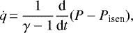
3.1 Circumstellar disk – model A
The interaction of SN ejecta with circumstellar disk is shown in Fig. 3. This type of interaction was studied previously, although for slightly different initial density profiles of the disk (Vlasis et al. 2016; McDowell et al. 2018; Kurfürst & Krtička 2019; Suzuki et al. 2019). The results of our simulations are similar to previous works, but we review our results here as a baseline for an interpretation of more complicated models. When the SN ejecta collide with the disk, a localized shock is formed and travels outward through the disk. In our model A, the ratio of disk to ejecta mass is relatively small, and as a result, the SN ejecta do not become significantly decelerated and continue expanding also in the equatorial direction. Still, shearing motion between the freely expanding polar ejecta and the slower shock interaction region leads to development of Kelvin–Helmholtz instability, which we see as a prominent vortex in the density plots. It is possible that the vortex would be less prominent in three-dimensional calculations, where the turbulence cascade is inverse compared to two dimensions. The overpressure in the shocked gas pushes the material above and below the equatorial plane, which we see as a slight overdensity just above and below the shock interaction region with uθ rapidly changing from negative to positive values. When the SN blast wave clears, these overdensities might be identified as expanding rings or cones. When comparing our results with previous works (Pejcha et al. 2017; Metzger & Pejcha 2017; McDowell et al. 2018; Kurfürst & Krtička 2019), we note that the overdensity either leads or lags behind the equatorial shock, which suggests that the detailed behavior depends on initial conditions like the vertical and radial density profile of the disk.
3.2 Colliding wind shells – models B
We show the interaction of SN ejecta with a colliding wind shell oriented toward the progenitor (model B1) in Figs. 4 and 5. This simulation was performed with a wider range of θ to see the shock interaction over a greater length of the shell. The interaction shock first appears at the standoff point on the vertical axis and then propagates away to greater θ. The shell is first hit by the fast low-density SN ejecta, which do not have significant momentum to cause noticeable expansion along the z axis. But eventually, the shell buckles and we see SN ejecta expanding above the shell in a series of Rayleigh–Taylor plumes. As the shock interaction spreads laterally to higher θ, progressively larger fraction of the SN ejecta velocity is oriented along the shell rather than perpendicular to it. Consequently, SN ejecta interacting with the shell achieves large positive uθ, as seen in the bottom row of Fig. 4. We witness development of shearing instabilities along the shell, which is especially well seen at t = 450 days around ϖ ≈ 400 R⋆ in the plots of ρ, ur, and uθ. We expect that more realistic initial conditions with perturbations of the colliding wind shell (e.g., Calderón et al. 2020) would lead to a faster development of the instabilities. Finally, the bottom row of Fig. 5 shows the volumetric shock heating rate  . We can identify forward and reverse shocks that bound the banana-shaped shock interaction region. Between t = 300 and 400 days the peak of
  moves along the shell away from the axis, but at t = 450 days the standoff point is reached by denser parts of the SN ejecta and
  significantly increases for|θ|≲ π∕4.
In Fig. 6, we explore the hydrodynamics of SN ejecta colliding with a plane shell (model B2a) with a standoff point located at the same distance as in model B1. The development of the instabilities is similar to model B1 in the sense that Rayleigh–Taylor plumes appear above the shell close to the z axis and Kelvin–Helmholtz vortices develop along the shell at larger ϖ. We also see a plume traveling above the shell back to the axis of symmetry with negative uθ, as shown in the middle row of Fig. 6. This plume is caused by low-density regions in the initial density distribution of the shell, which is an artificial feature discussed in Sect. 2.2.4. This material has low density and does not show high  , which implies that its observational consequences might be minor.
In Fig. 7, we show the same geometry configuration as in Fig. 6, but with a shell positioned significantly closer to the SN progenitor (model B2b). The evolution for the closer shell proceeds somewhat differently than for the shell positioned farther away. Due to the proximity of the shell to the SN progenitor, the high-momentum part of the ejecta hits the shell within the simulation time and the SN ejecta is able to break through the shell. We see that the denser parts of the SN ejecta become somewhat equatorially flattened, but the expansion generally continues in all directions. The interaction of the ejecta with the shell causes the formation of a thin filamentary overdensity, which winds in a complicated pattern in the outer regions of the polar ejecta. Similar but not identical filamentary pattern is seen also in the volumetric shock heating rate in the bottom row. We expect that in three-dimensional simulations or with corrugated initial density distribution of the shell, the filamentary structure would be less organized and perhaps completely dispersed. We expect that this region would still exhibit mixing and shock heating. Although there is noticeable shock heating around the filaments, the peak of  concentrates in areas where the shell is hit by SN ejecta with sufficiently high momentum to destroy the shell at that position. Finally, we expect that hydrodynamics in the case of a more distant shell (Fig. 6) would eventually resemble the behavior seen in Fig. 7 if the simulation was followed to later times and over larger domain sizes.
In Fig. 8, we illustrate the hydrodynamical evolution for a colliding wind shell oriented away from the SN progenitor (model B3). SN ejecta breaks through the shell near the standoff point on the z axis and we witness instabilities and shock heating as the ejecta propagates in the polar direction, similarly to models B1 and B2b. At greater distances from the SN progenitor, the shell becomes almost parallel with the radial direction and the shock interaction does not occur there as the fast ejecta sweep around. As a result,  remains high only relatively close to the progenitor. Ultimately, the shell will be destroyed as the bulk of the shocked region accelerates and moves outward, but we do not see this happening within the duration of simulation of model B3.
Finally, we point out several differences between SN ejecta interaction with a circumstellar disk and a colliding wind shell. In the case of disk interaction, the shock was localized primarily in the disk and only moved radially due to its bulk motion. In other words, the system could be described with two components: freely expanding SN ejecta in the polar direction with relatively small perturbations such as the overdense shoulder above and below the shocked region and the associated Kelvin–Helmholtz vortex, and strong shock propagating in the equatorial plane. Each of these components could be easily approximated with a separate spherically symmetric calculation. Indeed, we verified that the evolution near the equatorial plane could be relatively well described by a SNEC simulation with spherically symmetric CSM density distribution. Interaction with the colliding wind shell is fundamentally different, because the shocked region moves not only due to its bulk motion, but also because different parts of the shell get hit by different parts of the SN ejecta at different times. Although this type of interaction could be described as a superposition of a large number of collisions at progressively increasing radii, our simulations reveal that hydrodynamical instabilities are more vigorous than for the disk and effectively couple together evolution at different locations on the shell. When viewed fromthe SN progenitor, colliding wind shells can subtend much larger fraction of the solid angle than a circumstellar disk, which means that proportionally larger fraction of SN ejecta eventually significantly interacts with the CSM.
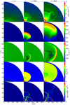 |
Fig. 3 Stages in the evolution of SN ejecta interacting with circumstellar disk (model A). The columns show snapshots at times t = 0, 200, and 400 days. Each row shows different quantity, from top to bottom: density ρ, radial velocity ur, polar velocity uθ, temperature T, and shock heating rate |

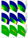 |
Fig. 4 Stages in the evolution of SN ejecta interacting with a colliding wind shell oriented to the SN progenitor (model B1). The columns show snapshots at times t = 300, 400, and 450 days. Each row shows different quantity, from top to bottom: density ρ, radial velocity ur, and polar velocity uθ. The remaining quantities are shown in Fig. 5. Animated version of the two combined figures is available as the movie B1. |
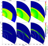 |
Fig. 5 Continuation of Fig. 4. Top row: temperature T
and bottom row: shock heating rate |

3.3 Bipolar nebula – model C
In Fig. 9, we show the hydrodynamical evolution of SN ejecta colliding with a bipolar nebula modeled after the Homunculus, but with smaller spatial scale and lower total mass (model C). We see that SN ejecta is deformed to resemble the original CSM shape. Since the lobes completely enclose the progenitor, the SN ejecta cannot pass around the denser parts of the CSM to expand freely in some direction (unlike the case of the circumstellar disk). As a result, we see reflected waves of the material propagating back into the regions within the original lobes, which is particularly noticeable in the plots of the density. Higher CSM density near the equator gives rise to a shocked region that is somewhat similar to the features seen in model A. Due to the complicated CSM geometry, various hydrodynamical instabilities are not as easy to localize as in the simpler geometries.
4 Implications for observations
Different CSM configurations result in qualitatively different hydrodynamical behavior in our simulations. We are now interested in finding observables, or their combinations, that would allow us to distinguish between different CSM geometries. We provide estimates of observable signatures for light curves (Sect. 4.1), late-time spectral line profiles (Sect. 4.2), and polarization (Sect. 4.3). We discuss implications for some observed SNe in Sect. 4.4.
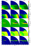 |
Fig. 6 Stages in the evolution of SN ejecta interacting with a planar shell located farther away from the progenitor (model B2a). The columns show snapshots at times t = 300, 400, and 450 days. The symbols and quantities are the same as in Fig. 3. Animated version of this figure is available as the movie B2a. |
4.1 Light curves
Without self-consistent treatment of radiation and hydrodynamics, we cannot make quantitative predictions for specific CSM properties, but we can investigate general trends using simpler semi-analytic models. In estimating the radiative luminosity, we must determine whether the optical depth to the radiative shock is relatively small and the instantaneous luminosity is proportional to the shock power, or whether the optical depth is large and the shock radiation diffuses out through a reprocessing layer. In bottom rows of Figs. 3–9, we overplot on the volumetric shock heating rate contours of electron scattering optical depths from two different sightlines under the assumption that the region is completely ionized. If the majority of the shock power is contained within a contour, the diffusion approximation is more appropriate than optically-thin treatment. Our estimate of the photosphereis very rough because we ignore other temperature- and density-dependent sources of opacity. For example, radiative shock can keep its vicinity ionized for a longer time and thus prevent hydrogen recombination and a drop of optical depth (e.g., Smith 2013b, 2017; Smith et al. 2015; Metzger & Pejcha 2017; Andrews & Smith 2018; Margutti et al. 2019). We thus consider both possibilities that the shock power is either instantaneously converted to optical radiation (Sect. 4.1.1) or it diffuses out of optically-thick envelope (Sect. 4.1.2).
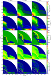 |
Fig. 7 Stages in the evolution of SN ejecta interacting with a planar shell located closer to the progenitor (model B2b). The columns show snapshots at times t = 300, 400, and 450 days. The symbols and quantities are the same as in Fig. 3. Animated version of this figure is available as the movie B2b. |
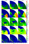 |
Fig. 8 Stages in the evolution of SN ejecta interacting with a colliding wind shell oriented away from the progenitor (model B3). The columns show snapshots at times t = 300, 400, and 450 days. The symbols and quantities are the same as in Fig. 3. Animated version of this figure is available as the movie B3. |
4.1.1 Shock power as a function of time
In the optically-thin case, the SN luminosity LSN is approximately proportional to the shock heating rate  of the radiative shock,
  , and we thus discuss the behavior of
  . We calculate
  numerically by integrating the volumetric shock heating rate
  given by Eq. (8) over the simulation volume
 (9)
(9)
Solid lines in the upper panel of Fig. 10 show the time evolution of  in our simulations. The dashed line corresponds to analytical calculation of shock power in the case of shock interaction with stellar wind (lower line) and circumstellar disk (upper line). Details of the calculation are given in Appendix A.
We see from Fig. 10 that  tracks the CSM density encountered by the shock. Model A (circumstellar disk) exhibits gradual decrease in
  , because the shock slows down as it sweeps up more mass of the disk. For models B1 (colliding wind shell oriented to the SN progenitor) and B2a (distant planar shell) in the first 200 days, the shock heating rate stays at ≈ 3 × 1039 ergs s−1, which is caused by the SN ejecta colliding with the spherically symmetric stellar wind. Later,
  increases gradually as a larger fraction of the SN ejecta interacts with the CSM. The rise in
  exhibits wiggles of ≲10%. For models B2b (close planar shell) and B3 (colliding wind shell oriented away from the SN progenitor), we see a fast rise in
  as the dense parts of the SN ejecta hit the nearby CSM at early times, which is followed by a gradual decline as progressively more distant regions of CSM are shocked. These models also exhibit fluctuations on a similar level to B1 and B2a. We expect that the shock heating rates of models B could exhibit potentially larger fluctuations with more realistic initial conditions that take into account corrugation of the colliding wind shells. Model C (bipolar nebula) presents the most complicated behavior with several high-amplitude bumps and wiggles caused by multiple shells in the CSM.
The shock power is also a useful quantity to compare numerical results with analytic estimates and with previous results on the same problem. Focusing on model A in the top panel of Fig. 10, we see that for most of the time the numerical results closely match the analytical predictions elaborated in Appendix A. Apart from the initial transient, a small disagreement is seen at approximately 70 days when numerical results give higher  than analytical estimates and after 400 days when the numerical
  is slightly lower than the analytical ones. Similar pattern is seen in Fig. 4 of McDowell et al. (2018). This suggests that our results are in agreement with those of McDowell et al. (2018) and that the realistic initial profile of the SN ejecta has relatively small effect on the outcome compared to the broken power-law used in analytical estimates and by McDowell et al. (2018).
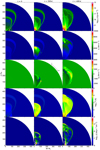 |
Fig. 9 Stages in the evolution of SN ejecta interacting with bipolar lobes (model C). The columns show snapshots at times t = 0, 200, and 400 days. The symbols and the quantities are the same as in Fig. 3. Animated version of this figure is available as the movie C. |
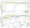 |
Fig. 10 Estimates of light curves from our simulations. Top: shock heating rate
|


4.1.2 Shock power as an internal power source
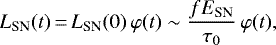
To estimate light curves under the assumption of shocks deeply embedded in the ejecta, we follow the semianalytic calculation of SN bolometric light curves introduced by Arnett (1980, 1982). We adopt the diffusion timescale τ0 ∝ κMSN∕RSN, where κ is the (Thomson) opacity (κ ≈ 0.34 cm2 g−1), MSN is the total mass of material that is involved in the explosion (ejecta + CSM), and ESN is the SN explosion energy, the hydrodynamical time τh = R⋆∕vSN (where we use vSN as an averaged maximum velocity of the forward shock front at the specified time), and the effective light curve timescale 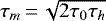 (Arnett 1982). The SN luminosity is then determined by
 (10)
(10)
where f is numerical factor (ratio of the initial thermal energy Eth(0) to the total energy ESN; we may relevantly choose f = 0.5). The dimensionless function φ(t) is (Chatzopoulos et al. 2012; McDowell et al. 2018)
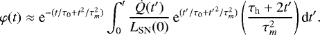 (11)
(11)
In the bottom panel of Fig. 10, we show the resulting time evolution of LSN. We see that taking into account diffusion converts  into gradually rising light curves with bumps and wiggles smoothed out, although model C retains some of the small scale structure. However, we do not see any light curve feature that would allow us to distinguish between different CSM geometries and different radial density profiles of spherically symmetric CSM.
Finally, we emphasize that shock interaction in our models is not occurring over the full solid angle of the SN ejecta. As a result, the part of the SN ejecta not interacting with the CSM will radiate similarly to a normal SN. This could lead to two-component light curves, similarly to what was suggested for luminous red novae (Metzger & Pejcha 2017) or kilonovae (e.g., Kasen et al. 2017). To illustratethis point, we show in the bottom panel of Fig. 10 theoretical light curve of a SN powered by the decay of 0.28 M⊙ of radioactive nickel. This light curve was obtained by using a different form of  in Eq. (11). We see that for models B1 and B2a, the CSM is positioned sufficiently far away from the progenitor so that the observed light curve would likely have a first recombination/radioactivity powered peak, followed by second peak powered by shock interaction. For the remaining models, the CSM is so close and so dense that the shock interaction dominates.
4.2 Spectral line profiles
Spectral line profiles can provide more insight into the ejecta geometry than disk-integrated light curves. However, calculating spectral lineprofiles in rapidly and differentially expanding medium out of local thermodynamic equilibrium is a complicated problem, which we do not attempt to solve here. Our goal is to provide guidance for how observed spectral line profiles relate to different CSM geometries. We are mostly interested in obtaining estimates of line profiles at late times, when the SN ejecta should be nearly transparent for radiation.
We obtain approximate line profiles by calculating volume-weighted histograms of line-of-sight velocities ulos for θ = 0, π∕4, and π∕2. The geometry of the problem is illustrated in Fig. 11. Our approach follows the simple examples in Jerkstrand (2017). We neglect absorption within the ejecta and assume that the emissivity does not depend on local density and temperature. Furthermore, we excise dense inner parts of the SN envelope, which correspond to the helium core. We determined approximate helium core radii with SNEC to be 8.6 × 1014 cm ≈ 12 R⋆ at 100 d, 1.8 × 1015 cm ≈ 25 R⋆ at 200 d, 2.6 × 1015 cm ≈ 36 R⋆ at 300 d, and 3.3 × 1015 cm ≈ 46 R⋆ at 400 d. Since our simulations are axisymmetric, we extend the dimensionality and add the azimuthal dependency by dividing each quadrant of the model to 24 azimuthal (ϕ-direction) intervals. More details of the calculation of uLOS are shown in Fig. 11. The resulting uLOS distributions are binned to approximately 360–960 bins within the total velocity range of ≈ ± 104 km s−1.
In order to build understanding of the spectral line profiles and to test our method, we first calculated the velocity distributions for simple configurations such as a homogeneous expanding sphere with constant density and homologous radial velocity profile. This configuration has the expected parabolic shape (Jerkstrand 2017). We then continued by adding artificial polar velocity components of different magnitudes. We also tested the more realistic case of spherically symmetric expanding SN without CSM with the input parameters corresponding to the progenitor parameters of our models. Finally, we address the issue of how to distinguish between the SN ejecta and the unshocked CSM. The unshocked CSM has typically much lower velocities than the SN ejecta and would contaminate only the bins near uLOS ≈ 0. We manually remove most of this effect, but caution should be taken when interpreting results near uLOS ≈ 0.
In Fig. 12, we show the calculated histograms of line-of-sight velocities for our models at a range of times and for three lines of sight, θ = 0, π∕4, and π∕2. Velocity for even higher viewing angles can be obtained by mirroring the lines in Fig. 12 around zero, for example, for θ = 3π∕4 the velocity distribution would look like for θ = π∕4 but with uLOS →−uLOS. We note that at later times the fastest SN ejecta have already left our computational grid and therefore the histograms are effectively cut at certain value of |uLOS|. The velocity profiles are always symmetric around uLOS for θ = π∕2, because the CSM distributions are rotationally symmetric around the z axis.
For model A (circumstellar disk) and θ = 0 (looking from the top side of Fig. 3), we see the expected pattern of two peaks located symmetrically at high positive and negative uLOS. The double-peaked pattern is less expressed from θ = π∕4 and not visible from θ = π∕2, because the velocity asymmetry is not aligned with the line of sight.
Models of the B series exhibit the greatest asymmetry between positive and negative uLOS, because the colliding wind shell is positioned on one side of the progenitor. In model B1, after the interaction starts at t ≳ 250 days, negative uLOS is suppressed because the material moving toward the observer is intercepted by the colliding wind shell. The shell is curved toward the progenitor and blocks ejecta over a wide range of solid angles and spatial scales. As a result, the suppression of negative uLOS is relatively smooth. In model B2a, the fastest ejecta with small momentum are completely deflected by the shell. As a result, there is a sharp drop in the distribution for negative uLOS and θ = 0. For θ = π∕4, the distribution is smoother and similar to model B1. Model B2b has the shell positioned closer to the SN, which means more time for the development of hydrodynamical instabilities. As a result, the velocity distribution for t ≲ 250 days is smooth and similar to model B2a but becomes rougher as the instabilities develop at later times. The peak at uLOS < 0 that gets relatively stronger over time arises from the ejecta that have broken through the shell and continue to expand toward the observer. Model B3 is qualitatively similar to B2b except that the ejecta that break through the standoff point of the shell are moving slower and therefore the peak at negative uLOS is weaker. Interestingly, even at late times, the distribution for θ = π∕4 remains nearly symmetric. To summarize, interactions with colliding wind shells lead to asymmetric multipeaked velocity distributions, where the relative strengths of the red and blue wings depend on the viewing angle and evolve in time. In some cases, the strongest peaks evolve from the blue to the red side or in the opposite way.
Finally, model C exhibits multiple peaks symmetrically positioned at positive and negative uLOS, because the bipolar nebula has mirror symmetry with respect to the z = 0 plane. Despite a very different CSM distribution, the uLOS distributions resemble the circumstellar disk in model A, albeit with a number of smaller peaks at intermediate velocities.
 |
Fig. 11 Schematic picture of the directions when calculating line-of-sight velocity distributions. |
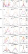 |
Fig. 12 Line-of-sight velocity distributions for our models. Each row corresponds to a different model, labeled on the left, and each column represents different viewing angle θ. Colored lines are results for different simulation times with legend given in the plot. The distributions are normalized to ensure clarity of the presentation and hence we do not display units on the vertical axes. The distributions are plotted on a linear scale. Some of the features around |uLOS | ≈ 0 are an artifact of subtraction of CSM that has not collided with the SN ejecta. The black dash-dotted line in the middle panel of model A illustrates the 400 d lower resolution model. |
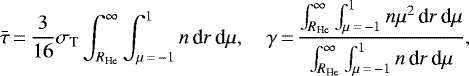
Values of the shape factor γ, averaged optical depth  , and the polarization degree PR for the models at four times, t = 100, 200, 300, and 400 d.
4.3 Polarization signatures
We estimate the polarization degree PR of the SN ejecta using the analytical prescriptions of Brown & McLean (1977) and Brown et al. (1978), which were derived under the assumption of Thomson scattering in an optically thin envelope irradiated by a central source. These approximations are certainly very crude for SN ejecta at late times, but allow us to get at least a relative assessment of the asphericity induced by the different CSM geometries. The polarization degree is given by
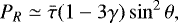 (12)
(12)
where θ is the inclination with the convention used in this paper, namely θ = 0 when viewed pole-on and θ = π∕2 when viewed equator-on. The averaged Thomson scattering optical depth  of the envelope and the shape factor γ are
 (13)
(13)
where σT is the Thomson scattering cross-section, n(r, μ) is the electron number density, and μ = cos θ. Assuming complete ionization of a pure hydrogen envelope, the electron number density is n(r, μ) = ρ(r, μ)∕mH, where mH is the mass of hydrogen atom. Equation (13) implies γ = 1∕3 for any spherically symmetric distribution, while γ < 1∕3 (PR > 0) in case of oblate, and γ > 1∕3 (PR < 0) in case of prolate mass distributions (Brown & McLean 1977; Brown et al. 1978). We eliminate the helium-dominated core from the calculation to emphasize the asphericity of the envelope and we denote the radius of the helium core as the lower limit of radial integration, RHe, in Eq. (13). We determined RHe in the same way as in Sect. 4.2.
Our results are shown in Fig. 13 and listed for four selected times, t ≈ 100, 200, 300, and 400 days, in Table 1. First, we look at models B1 and B2a at 100 days, where our numerically calculated PR is ≈ 0.03%. We would expect the bulk of the ejecta to be spherically symmetric with PR = 0 at this timebecause the SN ejecta have not reached the CSM at this epoch. Consequently, PR ≈ 0.03% roughly corresponds to the numerical noise of our polarization estimates. Looking now at the results, we see that models A and C have negative PR reaching about 2% at the end of our simulations. Polarization implies prolate distributions, which is caused by deflection of SN ejecta to polar regions by circumstellar disk (model A) or dense equatorial waist (model C). Models B1, B2a, and B2b exhibit positive PR, which remains low, PR ≲ 0.5%, at late times. Naturally, these models have oblate mass distribution because the colliding wind shell deflects material to the equatorial plane. Finally, model B3 reaches PR ≈−0.6%, which suggests prolate mass distribution likely caused by SN ejecta interaction near the standoff point.
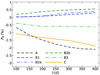 |
Fig. 13 Evolution of relative polarization degree for our models. Values at selected times are given in Table 1. |
4.4 Comparison with observed supernovae
The disk-integrated quantities estimated from our simulations broadly agree with what is observed: our approximate light curves in Fig. 10 peak around 1042 –1043 ergs s−1 and evolve slowly similarly to some observed overplotted in the same figure. The peak luminosity and the slope of the theoretical light curves depend on the CSM properties, which we do not systematically vary in this work. The actual light curve could also be a combination of radioactively-powered component (schematically indicated by the thin solid black line in the bottom panel of Fig. 10) and the shock interaction component calculated in one of our models. The polarizations in Table 1 match the continuum polarizations of 1–3% observed in interacting SNe (e.g., Leonard et al. 2000; Bilinski et al. 2018). However, these quantities depend on unconstrained parameters like density profile or inclination and therefore do not provide a clear-cut signature differentiating between CSM geometries. Consequently, we focus on the line-of-sight velocity distributions as a proxy for late-time spectral line profiles. There are a number of interacting SNe with late-time spectral line profiles implicating aspherical CSM. Few recent examples include SN2007od (Andrews et al. 2010; Inserra et al. 2011), SN2012ab (Bilinski et al. 2018), SN2013L (Andrews et al. 2017; Taddia et al. 2020), SN2013ej (Bose et al. 2015; Huang et al. 2015; Yuan et al. 2016; Mauerhan et al. 2017), SN2014G (Terreran et al. 2016), SN2014ab (Bilinski et al. 2020), iPTF14hls (Andrews & Smith 2018), KISS15s (Kokubo et al. 2019), SN2017eaw (Szalai et al. 2019; Weil et al. 2020), and SN2017gmr (Andrews et al. 2019). Typically, double-peaked line profiles are attributed to disk- or torus-like geometry (e.g., Gerardy et al. 2000; Jerkstrand 2017). Double-peaked profile is also prominently seen in our model A in Fig. 12. A boxy, flat-topped profile with a possibility of double-peaked horns was argued to arise from bipolar lobes similar to what is seen in η Car. An example is an eruption of a SN impostor UGC 2773-OT (Smith et al. 2016). Our model C in Fig. 12 remotely resembles such profiles, but with relatively strong dependence on the viewing angle.
Suppression of the red side of a nebular spectral line is often attributed to dust formation, which more effectively blocks the light coming from the more distant receding side of the SN (e.g., Lucy et al. 1989; Sugerman et al. 2006; Smith et al. 2008). However, in some cases the observations indicate that there is a genuine asymmetry in the SN, or more specifically, the SN lacks either rotational symmetry with respect to an axis or mirror symmetry with respect to an equatorial plane. One example is SN2013L, where Andrews et al. (2017) observed the same blueshifted asymmetric line profile in Hα and Paβ that cannot be explained by internal wavelength-dependent dust obscuration. Even more striking example is PTF11iqb analyzed by Smith et al. (2015). In the first few days after the explosion, PTF11iqb showed Wolf–Rayet-like spectral features likely arising from flash-ionized CSM of the inner wind of its red supergiant progenitor. For the next ~ 100 days, the spectrum and light curve resembled a normal Type II-P SN. In the nebular phase, Hα emission initially showed a blueshifted peak, but after ~500 days a redshifted peak appeared and eventually dominated Hα emission. In addition, Hα emission exhibited several smaller bumps and peaks. Smith et al. (2015) could not explain the late evolution by disappearance of the dust and instead argued for a disk- or torus-like CSM with enhanced density on the more distant redshifted side of the SN.
Instead of an azimuthally-asymmetric disk, there are several reasons why an interaction with a colliding wind shell could explain PTF11iqb. First, the colliding wind shell occurs only on one side of the SN and naturally satisfies the condition of equatorial plane asymmetry. Second, the Wolf–Rayet-like signatures could arise either in the dense slow wind of the progenitor or in the density enhancement in the colliding wind shell, similarly to what Kochanek (2019) suggested for SN2013fs. Third, the standoff point of the colliding wind shell might be located relatively close to the SN, which means that the CSM interaction begins early with a sharp peak and continues to gradually decrease over time (models B2b and B3 in Fig. 10). Fourth, since the shock interaction occurs only over a small fraction of the solid angle, the shock can be embedded in the ejecta to hide the narrow lines and produce a relatively normal-looking plateau, similarly to what is argued for a disk-like CSM. Finally, the evolution of blue and red peaks of nebular Hα resembles models B2b and B3 viewed either from θ = 0 or θ = 3π∕4 (equivalent to θ = π∕4 with velocity distribution flipped around the origin).
There are other events, where colliding wind shell might be a better explanation for the observations than circumstellar disk. Following the reasoning of Smith et al. (2015), SN1998S might be explained by a similar geometry as PTF11iqb, but viewed from a different viewing angle. Recently, Bilinski et al. (2020) presented observations of SN2014ab, which show nearly identical Hα and Paβ profiles withstrong blueshifted component, implying a lack of symmetry between the near and far side of the SN. The event shows little polarization suggesting circular symmetry from our line of sight. Bilinski et al. (2020) argued that the lack of polarization is due to our viewing angle near the axis of symmetry (for example, looking from θ = 0 at our model A) and the spectral line asymmetry is due to internal absorption in the shock interaction region, which hides its farther receding side. Interestingly, our colliding wind models consistently predict asymmetric velocity distributions from most viewing angles and noticeably smaller polarization degrees than circumstellar disk or bipolar lobes models. Although the observed luminosities of PTF11iqb and SN2014ab are somewhat smaller than what we predict in our models (bottom panel of Fig. 10), we expect that better agreement could be reached by varying some of the parameters of our models. For example, lowering α in Eq. (7) would decrease the surface density and total mass of the colliding wind shell while maintaining the shape, which would lead to lower luminosity from the shock and better agreement with the observed light curves.
5 Conclusions
We have performed two-dimensional axisymmetric hydrodynamic simulations of spherically symmetric SN ejecta colliding with aspherical CSM. The main improvements over the previous works are realistic initial density and velocity profiles of the SN ejecta and a wider range of CSM geometries. In particular, for the first time we studied shock interaction with a colliding wind shell in a binary star and compared the results to SN interactions with circumstellar disk and bipolar lobes. The typical CSM masses on our computational grid are 10−3 to 10−2 M⊙. Snapshots of density, radial and polar velocity, temperature, and shock heating are summarized in Figs. 3–9 and in Sect. 3. All our models exhibit deceleration of the expanding SN ejecta by the CSM and the ensuing deflection of the explosion to the directions of the least resistance. The hydrodynamics involves oblique and deflected shocks and their clustering, shearing motions accompanied by Kelvin–Helmholtz instabilities, and shock propagation through density gradients leading to Rayleigh–Taylor-like instabilities. We saw that the expanding material often wraps around the denser parts of the CSM.
Based on our hydrodynamical simulations, we estimated three observables of CSM interaction in SNe: the shock power and the related bolometric luminosity, distribution of line-of-sight velocities as a proxy for late-time spectral line profiles, and the degree of polarization. The shock energy deposition closely traces the course of the interaction and reaches up to 1044 ergs s−1. If embedded inside an optically thick envelope, the energy generated by the shock gradually diffuses out of the SN ejecta, which we estimate using an analytic one-zone model. The resulting bolometric luminosities are in the range of 1042 –1043 ergs s−1 (Fig. 10 and Sect. 4.1), which is in the range of what is observed in Type IIn SNe (Fig. 1). The time dependence of shock power shows short-term fluctuations or peaks with amplitudes ≲ 10%, which get smoothed and erased if the shocks are embedded in and reprocessed by the SN envelope. Interaction with bipolar lobes, where the CSM is structured in several concentric shells, leads to more prominent fluctuations. Our models thus do not readily explain the bumps and wiggles observed in some interacting SNe (Fig. 1). Perhaps coupling radiation to the hydrodynamics would allow for easier escape of the shock-generated radiation through the crevices created by the hydrodynamic instabilities.Alternatively, the instabilities could be amplified by more realistic initial conditions taking into account the clumpiness of the CSM (e.g., Calderón et al. 2016, 2020).
The distribution of line-of-sight velocities (Fig. 12 and Sect. 4.2) has the greatest discriminating power between different CSM geometries studied here. Our models show the expected double-peaked profile for the circumstellar disk and symmetric multipeaked flat-top profile for the bipolar lobes. The colliding wind shell is positioned only on one side of the SN and could naturally explain blue–red asymmetry of late-time line profiles, which cannot be readily explained by internal obscuration due to dust. An example of such object is PTF11iqb (Sect. 4.4 and Smith et al. 2015). The small solid angle subtended by the interaction regions could lead to engulfment of the shock by the SN ejecta, which might hide the narrow lines and make the shock essentially an internal power source inside the envelope.
Our estimates of the degree of polarization (Table 1 and Sect. 4.3) give values similar to what is observed (e.g., Dessart & Hillier 2011; Gal-Yam 2019). CSM in the form of circumstellar disk and bipolar lobes leads to prolate shape of the ejecta and maximum polarization on the level of 1–2%. Interaction with a colliding wind shell leads to smaller amounts of polarization ≲ 0.5% and usually oblate shapes. Despite these differences, the estimates of polarization degree of our models are not sufficiently different from each other to discriminate between different CSM geometries on their own, especially when taking into account unconstrained degrees of freedom such as the viewing angle and parameters of the CSM density distributions.
To summarize, we performed hydrodynamic-only simulations to explore and widen the range of CSM geometries considered for interacting SNe. We recovered expected results for circumstellar disk and bipolar lobes. Our results suggest thatcolliding wind shells are particularly promising for explaining more complicated asymmetries and time evolution observed in some SNe. Occurrence rates of colliding wind shells around SN progenitors should be estimated, for example, based on the binary population synthesis models (e.g., Eldridge et al. 2008). More sophisticated simulations including proper treatment of radiation should be performed to provide more realistic predictions for observations. With sufficiently developed theory to robustly detect and characterize colliding wind shells interacting with SN explosions, it might be possible to characterize binary companions to SNe in a new way. For example, modeling of the observed light curves and spectral line profiles might provide the time when the shock reaches the standoff point of the colliding wind shell, which is proportional to the physical distance from the progenitor, as well as the orientation of the shell. With these estimates, we could infer the separation between the two binary components and the wind momentum of the companion, which would constrain its evolutionary state.
Movies
Movie of Fig. 3 Access Supplementary Material
Movie of Fig. 4 Access Supplementary Material
Movie of Fig. 6 Access Supplementary Material
Movie of Fig. 7 Access Supplementary Material
Movie of Fig. 8 Access Supplementary Material
Movie of Fig. 9 Access Supplementary Material
Acknowledgements
We thank to Dr. Milan Prvák for technical support and useful improvements in computational process and in preparation of the draft of this paper. P.K. and O.P. were supported by the grant Primus/SCI/17. O.P. was additionally supported by Horizon 2020 ERC Starting Grant “Cat-In-hAT” (grant agreement #803158) and INTER-EXCELLENCE grant LTAUSA18093 from the Ministry of Education, Youth, and Sports. This work was also supported by the grant GAČR 18-05665S. Computational resources were supplied by the project “e-Infrastruktura CZ” (e-INFRA LM2018140) provided within the program Projects of Large Research, Development and Innovations Infrastructures.
Appendix A: Analytical scaling of SN-wind and SN-disk interaction
Here we summarize the equations that are used to analytically estimate the power produced by a strong shock that propagates through the stellar wind or through analytically scaled CSM configurations like a circumstellar disk. Results of these estimates were used in Sect. 4.1 and Fig. 10. We start by constructinganalytic description of the density profiles of the SN ejecta and the CSM. For SN ejecta, we follow the broken power law defined by Chevalier & Soker (1989) with an inner flatter region and an outer steeper region. The distance of the transition point between the two regions and the velocity at this point are related as Rtr = vtrt. The density of a spherically symmetric ejecta is  for r < Rtr,
  for Rtr < r < RSN, where RSN = vmax t is the velocity of the outermost layer of the expanding SN ejecta. The density and velocity of the transition point are
![Mathematical equation: \begin{align*}\rho_{\text{tr}}\,{=}\,\frac{(3-\delta)(n-3)}{4\pi\,(n-\delta)} \frac{M_{\text{ej}}}{R_{\text{tr}}^{3}},\quad \varv_{\text{tr}}\,{=}\,\left[\frac{2(5-\delta)(n-5)}{(3-\delta)(n-3)} \frac{E_{\text{ej}}}{M_{\text{ej}}}\right]^{1/2}, \end{align*}](/articles/aa/full_html/2020/10/aa39073-20/aa39073-20-eq46.png) (A.1)
(A.1)
where Mej and Eej are mass and energy of SN ejecta, respectively, while ρej = 0 for r > RSN. The inner density slope δ ≃ 0–1 and the outer density slope n ≃ 10 is expected for SNe Ib/Ic and SNe Ia (Matzner & McKee 1999; Kasen 2010) while n ≃ 12 is commonly accepted for RSGs (Matzner & McKee 1999).
We describe the density profile ρsw(r) of spherically symmetric circumstellar environment (wind) in Eq. (5) and the density profile ρdisk(r, θ) of the thin circumstellar disk in Eq. (6) (cf. Kurfürst & Krtička 2019, cf. also Eq. (37) in Kurfürst et al. 2018). The total mass of the shocked SN ejecta and CSM, Msh, becomes
 (A.2)
(A.2)
where Rsh = vsht is the radius of the shock front. We integrate the second term in the right-hand side of Eq. (A.2) from the stellar radius R⋆ ≪ Rsh, because we assume the CSM is sweeped up to the radius Rsh, forming there a thin shell. We obtain
 (A.3)
(A.3)
where the constants  ,
,  and
and  , s and w are pre-explosion density slopes of wind and disk, respectively; for the meaning of base densities ρ0,wind and ρ0,disk, see Sect. 1 and Eq. (6) in Sect. 2.
Employing the shocked shell pressure force (scaled from Rankine-Hugoniot relations), assuming a strong shock and neglecting pre-explosion velocities of CSM,
![Mathematical equation: \begin{align*}\left[\rho_{\text{ej}}\left(\varv_{\text{SN}}-\varv_{\text{sh}}\right)^2- \left(\rho_{\text{sw}}+\rho_{\text{disk}}\right)\varv_{\text{sh}}^2\right]4\pi R_{\text{sh}}^2\,{=}\,M_{\text{sh}}\frac{\text{d}\varv_{\text{sh}}}{\text{d}t}, \end{align*}](/articles/aa/full_html/2020/10/aa39073-20/aa39073-20-eq52.png) (A.4)
(A.4)
and by substituting Eq. (A.3) and the shock velocity into Eq. (A.4), we obtain
![Mathematical equation: \begin{align*}&\frac{B_{\text{sn}}t^{n-3}}{R_{\text{sh}}^{n-2}}\left(\frac{R_{\text{sh}}}{t}- \frac{\text{d}R_{\text{sh}}}{\text{d}t}\right)^2 - \left(D_{\text{sw}} R_{\text{sh}}^{2-s}+ D_{\text{disk}}R_{\text{sh}}^{2-w} \right)\left(\frac{\text{d}R_{\text{sh}}}{\text{d}t}\right)^2\nonumber\\ &\quad =\left[ \frac{B_{\text{sn}}}{n-3}\left(\frac{t}{R_{\text{sh}}}\right)^{n-3}+ \frac{D_{\text{sw}}R_{\text{sh}}^{3-s}}{3-s}+ \frac{D_{\text{disk}}R_{\text{sh}}^{3-w}}{3-w}\right] \frac{\text{d}^2R_{\text{sh}}}{\text{d}t^2}. \end{align*}](/articles/aa/full_html/2020/10/aa39073-20/aa39073-20-eq53.png) (A.5)
(A.5)
Assuming the solution of Eq. (A.5) as a power law in the form Rsh (t) = Atα, we analytically evaluate the factor A for a shock wave that propagates through CSM. We write the explicit form of the power law solution for Rsh, sw and Rsh, disk, respectively,as
![Mathematical equation: \begin{align*}& R_{\text{sh,\,sw}}(t)\,{=}\,\left[\frac{(3-s)(4-s)}{(n-3)(n-4)} \frac{B_{\text{sn}}} {D_{\text{sw}}}\right]^{1/(n-s)}t^{(n-3)/(n-s)},\nonumber\\% \qquad & R_{\text{sh,\,disk}}(t)\,{=}\,\left[\frac{\left(\widetilde{H}+3-w\right)(3-w)}{(n-3)(n-4)} \frac{B_{\text{sn}}}{D_{\text{disk}}}\right]^{1/(n-w)}t^{(n-3)/(n-w)}, \end{align*}](/articles/aa/full_html/2020/10/aa39073-20/aa39073-20-eq54.png) (A.6)
(A.6)
where  (Eq. (6)). If we substitute n = 12, s = 2, w = 2, and
  , we get
  and
and  . We use here the approximation
  for analytical feasibility, even if
  is not a constant in general unless the disk temperature radially decreases as T ~ r−1 (cf. Kurfürst et al. 2014, 2018).
We estimate the shock power as the product of pressure force exerted by the shock on the unshocked material and the shock velocity (cf. McDowell et al. 2018),
 (A.7)
(A.7)
where Psh is the pressure behind the shock front that propagates through the stellar wind or the disk region, vsh is the corresponding shock velocity (that can be derived, e.g., from second Eq. (A.6)), and Ssh is the surface area of the shock in the wind or disk region. For a strong shock is the pressure Psh given by (Zel’dovich & Raizer 1967)
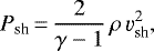 (A.8)
(A.8)
where ρ is either ρwind (Eq. (5)) or ρdisk (Eq. (6)), simplified for the case of thin equatorial disk, θ ≈ π∕2. We can express the corresponding shock surface area simply as
 (A.9)
(A.9)
respectively.
Following these assumptions, we obtain the analytically estimated shock heating rate (shock power) for the disk angular region as
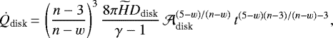 (A.10)
where  is the factor in square brackets in second Eq. (A.6). The shock heating rate
  for the spherically symmetric wind region is quite analogous; we may set a simple approximation
  , or we can calculate
  using Eq. (5). We also estimate the ratio
  , that is, what will be the contribution of the disk to the shock powered luminosity to that of the whole spherically symmetric CSM. If, for example, the parameters s = 2, w = 2, n = 7–12,
 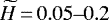 (see Eq. (A.6) for the meaning of the parameters), we obtain the ratio
 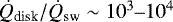 .
.
References
- Anderson, J. P. 2019, A&A, 628, A7 [NASA ADS] [CrossRef] [EDP Sciences] [Google Scholar]
- Andrews, J. E., & Smith, N. 2018, MNRAS, 477, 74 [Google Scholar]
- Andrews, J. E., Gallagher, J. S., Clayton, G. C., et al. 2010, ApJ, 715, 541 [Google Scholar]
- Andrews, J. E., Smith, N., McCully, C., et al. 2017, MNRAS, 471, 4047 [Google Scholar]
- Andrews, J. E., Sand, D. J., Valenti, S., et al. 2019, ApJ, 885, 43 [Google Scholar]
- Arcavi, I., Howell, D. A., Kasen, D., et al. 2017, Nature, 551, 210 [Google Scholar]
- Aretxaga, I., Benetti, S., Terlevich, R. J., et al. 1999, MNRAS, 309, 343 [Google Scholar]
- Arnett, W. D. 1980, ApJ, 237, 541 [Google Scholar]
- Arnett, W. D. 1982, ApJ, 253, 785 [Google Scholar]
- Bilinski, C., Smith, N., Williams, G. G., et al. 2018, MNRAS, 475, 1104 [Google Scholar]
- Bilinski, C., Smith, N., Williams, G. G., et al. 2020, MNRAS, in press [Google Scholar]
- Blondin, J. M., Lundqvist, P., & Chevalier, R. A. 1996, ApJ, 472, 257 [Google Scholar]
- Bose, S., Sutaria, F., Kumar, B., et al. 2015, ApJ, 806, 160 [Google Scholar]
- Braun, K., Baade, R., Reimers, D., & Hagen, H. J. 2012, A&A, 546, A3 [NASA ADS] [CrossRef] [EDP Sciences] [Google Scholar]
- Brown, J. C., & McLean, I. S. 1977, A&A, 57, 141 [NASA ADS] [Google Scholar]
- Brown, J. C., McLean, I. S., & Emslie, A. G. 1978, A&A, 68, 415 [NASA ADS] [Google Scholar]
- Calderón, D., Ballone, A., Cuadra, J., et al. 2016, MNRAS, 455, 4388 [Google Scholar]
- Calderón, D., Cuadra, J., Schartmann, M., et al. 2020, MNRAS, 493, 447 [Google Scholar]
- Chatzopoulos, E., Wheeler, J. C., & Vinko, J. 2012, ApJ, 746, 121 [Google Scholar]
- Chevalier, R. A. 1982, ApJ, 259, 302 [NASA ADS] [CrossRef] [Google Scholar]
- Chevalier, R. A., & Soker, N. 1989, ApJ, 341, 867 [Google Scholar]
- Chornock, R., Filippenko, A. V., Li, W., & Silverman, J. M. 2010, ApJ, 713, 1363 [Google Scholar]
- Chugai, N. N., & Danziger, I. J. 1994, MNRAS, 268, 173 [NASA ADS] [Google Scholar]
- Dessart, L., & Hillier, D. J. 2011, MNRAS, 415, 3497 [Google Scholar]
- Dessart, L., Audit, E., & Hillier, D. J. 2015, MNRAS, 449, 4304 [Google Scholar]
- Dessart, L., Hillier, D. J., Audit, E., Livne, E., & Waldman, R. 2016, MNRAS, 458, 2094 [Google Scholar]
- Eldridge, J. J., Izzard, R. G., & Tout, C. A. 2008, MNRAS, 384, 1109 [NASA ADS] [CrossRef] [Google Scholar]
- Fransson, C., Chevalier, R. A., Filippenko, A. V., et al. 2002, ApJ, 572, 350 [NASA ADS] [CrossRef] [Google Scholar]
- Gal-Yam, A. 2012, Science, 337, 927 [Google Scholar]
- Gal-Yam, A. 2019, ARA&A, 57, 305 [Google Scholar]
- Gayley, K. G., Owocki, S. P., & Cranmer, S. R. 1997, ApJ, 475, 786 [Google Scholar]
- Gerardy, C. L., Fesen, R. A., Höflich, P., & Wheeler, J. C. 2000, AJ, 119, 2968 [Google Scholar]
- Goldman, S. R., van Loon, J. T., Zijlstra, A. A., et al. 2017, MNRAS, 465, 403 [Google Scholar]
- González, R. F., Villa, A. M., Gómez, G. C., et al. 2010, MNRAS, 402, 1141 [Google Scholar]
- Guillochon, J., Parrent, J., Kelley, L. Z., & Margutti, R. 2017, ApJ, 835, 64 [Google Scholar]
- Heger, A., & Langer, N. 1998, A&A, 334, 210 [NASA ADS] [Google Scholar]
- Huang, F., Wang, X., Zhang, J., et al. 2015, ApJ, 807, 59 [Google Scholar]
- Hubová, D., & Pejcha, O. 2019, MNRAS, 489, 891 [Google Scholar]
- Inserra, C., Turatto, M., Pastorello, A., et al. 2011, MNRAS, 417, 261 [Google Scholar]
- Jerkstrand, A. 2017, Handbook of Supernovae, eds. A. W. Alsabti, & P. Murdin (Cham: Springer), 795 [Google Scholar]
- Kasen, D. 2010, ApJ, 708, 1025 [Google Scholar]
- Kasen, D., Metzger, B., Barnes, J., Quataert, E., & Ramirez-Ruiz, E. 2017, Nature, 551, 80 [Google Scholar]
- Kashi, A., & Soker, N. 2010, ApJ, 723, 602 [Google Scholar]
- Kee, N. D., Owocki, S., & ud-Doula, A. 2014, MNRAS, 438, 3557 [NASA ADS] [CrossRef] [Google Scholar]
- Kochanek, C. S. 2019, MNRAS, 483, 3762 [Google Scholar]
- Kokubo, M., Mitsuda, K., Morokuma, T., et al. 2019, ApJ, 872, 135 [Google Scholar]
- Kraus, M., Borges Fernandes, M., & de Araújo, F. X. 2007, A&A, 463, 627 [NASA ADS] [CrossRef] [EDP Sciences] [Google Scholar]
- Krtička, J., Owocki, S. P., & Meynet, G. 2011, A&A, 527, A84 [NASA ADS] [CrossRef] [EDP Sciences] [Google Scholar]
- Kurfürst, P., & Krtička, J. 2017, Appl. Math., 62, 633 [Google Scholar]
- Kurfürst, P., & Krtička, J. 2019, A&A, 625, A24 [CrossRef] [EDP Sciences] [Google Scholar]
- Kurfürst, P., Feldmeier, A., & Krtička, J. 2014, A&A, 569, A23 [NASA ADS] [CrossRef] [EDP Sciences] [Google Scholar]
- Kurfürst, P., Feldmeier, A., & Krtička, J. 2017, ASP Conf. Ser., 508, 17 [Google Scholar]
- Kurfürst, P., Feldmeier, A., & Krtička, J. 2018, A&A, 613, A75 [NASA ADS] [CrossRef] [EDP Sciences] [Google Scholar]
- Leonard, D. C., Filippenko, A. V., Barth, A. J., & Matheson, T. 2000, ApJ, 536, 239 [Google Scholar]
- Li, K.-L., Metzger, B. D., Chomiuk, L., et al. 2017, Nat. Astron., 1, 697 [Google Scholar]
- Lucy, L. B., Danziger, I. J., Gouiffes, C., & Bouchet, P. 1989, Supernovae, eds. G. Tenorio-Tagle, M. Moles, & J. Melnick (New York: Springer), 350, 164 [Google Scholar]
- Mackey, J., Mohamed, S., Gvaramadze, V. V., et al. 2014, Nature, 512, 282 [Google Scholar]
- MacLeod, M., Ostriker, E. C., & Stone, J. M. 2018, ApJ, 868, 136 [Google Scholar]
- Margutti, R., Metzger, B. D., Chornock, R., et al. 2019, ApJ, 872, 18 [Google Scholar]
- Matzner, C. D., & McKee, C. F. 1999, ApJ, 510, 379 [Google Scholar]
- Mauerhan, J. C., Smith, N., Silverman, J. M., et al. 2013, MNRAS, 431, 2599 [Google Scholar]
- Mauerhan, J. C., Van Dyk, S. D., Johansson, J., et al. 2017, ApJ, 834, 118 [Google Scholar]
- McDowell, A. T., Duffell, P. C., & Kasen, D. 2018, ApJ, 856, 29 [Google Scholar]
- Metzger, B. D., & Pejcha, O. 2017, MNRAS, 471, 3200 [Google Scholar]
- Moe, M., & Di Stefano, R. 2017, ApJS, 230, 15 [Google Scholar]
- Moriya, T. J., Blinnikov, S. I., Baklanov, P. V., Sorokina, E. I., & Dolgov, A. D. 2013, MNRAS, 430, 1402 [Google Scholar]
- Moriya, T. J., Förster, F., Yoon, S.-C., Gräfener, G., & Blinnikov, S. I. 2018, MNRAS, 476, 2840 [Google Scholar]
- Morozova, V., Piro, A. L., Renzo, M., et al. 2015, ApJ, 814, 63 [Google Scholar]
- Morris, T., & Podsiadlowski, P. 2007, Science, 315, 1103 [Google Scholar]
- Müller, T., Prieto, J. L., Pejcha, O., & Clocchiatti, A. 2017, ApJ, 841, 127 [Google Scholar]
- Nyholm, A., Sollerman, J., Taddia, F., et al. 2017, A&A, 605, A6 [NASA ADS] [CrossRef] [EDP Sciences] [Google Scholar]
- Okazaki, A. T. 2001, PASJ, 53, 119 [Google Scholar]
- Pandolfi, M., & D’Ambrosio, D. 2001, J. Comput. Phys., 166, 271 [Google Scholar]
- Patat, F., Taubenberger, S., Benetti, S., Pastorello, A., & Harutyunyan, A. 2011, A&A, 527, L6 [NASA ADS] [CrossRef] [EDP Sciences] [Google Scholar]
- Paxton, B., Bildsten, L., Dotter, A., et al. 2011, ApJS, 192, 3 [Google Scholar]
- Paxton, B., Cantiello, M., Arras, P., et al. 2013, ApJS, 208, 4 [NASA ADS] [CrossRef] [Google Scholar]
- Pejcha, O., & Prieto, J. L. 2015, ApJ, 806, 225 [Google Scholar]
- Pejcha, O., Metzger, B. D., & Tomida, K. 2016a, MNRAS, 455, 4351 [Google Scholar]
- Pejcha, O., Metzger, B. D., & Tomida, K. 2016b, MNRAS, 461, 2527 [Google Scholar]
- Pejcha, O., Metzger, B. D., Tyles, J. G., & Tomida, K. 2017, ApJ, 850, 59 [Google Scholar]
- Podsiadlowski, P., Joss, P. C., & Hsu, J. J. L. 1992, ApJ, 391, 246 [Google Scholar]
- Sana, H., de Mink, S. E., de Koter, A., et al. 2012, Science, 337, 444 [Google Scholar]
- Smith, N. 2011, MNRAS, 415, 2020 [Google Scholar]
- Smith, N. 2013a, MNRAS, 434, 102 [Google Scholar]
- Smith, N. 2013b, MNRAS, 429, 2366 [Google Scholar]
- Smith, N. 2014, ARA&A, 52, 487 [Google Scholar]
- Smith, N. 2017, Handbook of Supernovae, eds. A. W. Alsabti, & P. Murdin (Cham; Springer), 403 [Google Scholar]
- Smith, N., & McCray, R. 2007, ApJ, 671, L17 [Google Scholar]
- Smith, N., Foley, R. J., & Filippenko, A. V. 2008, ApJ, 680, 568 [Google Scholar]
- Smith, N., Silverman, J. M., Chornock, R., et al. 2009, ApJ, 695, 1334 [Google Scholar]
- Smith, N., Mauerhan, J. C., Cenko, S. B., et al. 2015, MNRAS, 449, 1876 [Google Scholar]
- Smith, N., Andrews, J. E., Mauerhan, J. C., et al. 2016, MNRAS, 455, 3546 [Google Scholar]
- Smith, N., Andrews, J. E., Rest, A., et al. 2018, MNRAS, 480, 1466 [Google Scholar]
- Steinberg, E., & Metzger, B. D. 2018, MNRAS, 479, 687 [NASA ADS] [Google Scholar]
- Stevens, I. R., Blondin, J. M., & Pollock, A. M. T. 1992, ApJ, 386, 265 [NASA ADS] [CrossRef] [Google Scholar]
- Stritzinger, M., Taddia, F., Fransson, C., et al. 2012, ApJ, 756, 173 [Google Scholar]
- Sugerman, B. E. K., Ercolano, B., Barlow, M. J., et al. 2006, Science, 313, 196 [Google Scholar]
- Suzuki, A., Moriya, T. J., & Takiwaki, T. 2019, ApJ, 887, 249 [Google Scholar]
- Szalai, T., Vinkó, J., Könyves-Tóth, R., et al. 2019, ApJ, 876, 19 [Google Scholar]
- Taddia, F., Stritzinger, M. D., Fransson, C., et al. 2020, A&A, 638, A92 [CrossRef] [EDP Sciences] [Google Scholar]
- Terreran, G., Jerkstrand, A., Benetti, S., et al. 2016, MNRAS, 462, 137 [Google Scholar]
- van Marle, A. J., Smith, N., Owocki, S. P., & van Veelen, B. 2010, MNRAS, 407, 2305 [Google Scholar]
- Vishniac, E. T. 1994, ApJ, 428, 186 [NASA ADS] [CrossRef] [Google Scholar]
- Vlasis, A., Dessart, L., & Audit, E. 2016, MNRAS, 458, 1253 [Google Scholar]
- Wang, L., & Wheeler, J. C. 2008, ARA&A, 46, 433 [Google Scholar]
- Weil, K. E., Fesen, R. A., Patnaude, D. J., & Milisavljevic, D. 2020, ApJ, 900, 11 [Google Scholar]
- Wilkin, F. P. 1996, ApJ, 459, L31 [Google Scholar]
- Yuan, F., Jerkstrand, A., Valenti, S., et al. 2016, MNRAS, 461, 2003 [Google Scholar]
- Zel’dovich, Ya. B., & Raizer, Yu. P. 1967, Physics of Shock Waves and High-Temperature Hydrodynamic Phenomena (Mineola, NY: Dover Publications, Inc.) [Google Scholar]
All Tables
Values of the shape factor γ, averaged optical depth , and the polarization degree PR for the models at four times, t = 100, 200, 300, and 400 d.
All Figures
|
Fig. 1 Comparison of light curves of five prominent long-lasting SNe II (after Nyholm et al. 2017). The photometry data are from Aretxaga et al. (1999), Stritzinger et al. (2012), Smith et al. (2009), Nyholm et al. (2017), Arcavi et al. (2017), and were obtained from the Open Supernova Catalog (Guillochon et al. 2017). We convert the r∕R magnitudes to bolometric L according to Eq. (1) in Nyholm et al. (2017), which applies constant zero bolometric correction. |
| In the text | |
|
Fig. 2 Initial profiles of selected hydrodynamic quantities. Black lines show the initial numerical profiles of density ρ, radial velocity ur, pressure P, and temperature T of the SN ejecta (gray region with 0.2 ≤ r∕R⋆ ≤ 1) and of the stellar wind in the close vicinity (r > R⋆). The red lineshows the initial analytical density profile described in Appendix A. |
| In the text | |
|
Fig. 3 Stages in the evolution of SN ejecta interacting with circumstellar disk (model A). The columns show snapshots at times t = 0, 200, and 400 days. Each row shows different quantity, from top to bottom: density ρ, radial velocity ur, polar velocity uθ, temperature T, and shock heating rate |
| In the text | |
|
Fig. 4 Stages in the evolution of SN ejecta interacting with a colliding wind shell oriented to the SN progenitor (model B1). The columns show snapshots at times t = 300, 400, and 450 days. Each row shows different quantity, from top to bottom: density ρ, radial velocity ur, and polar velocity uθ. The remaining quantities are shown in Fig. 5. Animated version of the two combined figures is available as the movie B1. |
| In the text | |
|
Fig. 5 Continuation of Fig. 4. Top row: temperature T
and bottom row: shock heating rate |
| In the text | |
|
Fig. 6 Stages in the evolution of SN ejecta interacting with a planar shell located farther away from the progenitor (model B2a). The columns show snapshots at times t = 300, 400, and 450 days. The symbols and quantities are the same as in Fig. 3. Animated version of this figure is available as the movie B2a. |
| In the text | |
|
Fig. 7 Stages in the evolution of SN ejecta interacting with a planar shell located closer to the progenitor (model B2b). The columns show snapshots at times t = 300, 400, and 450 days. The symbols and quantities are the same as in Fig. 3. Animated version of this figure is available as the movie B2b. |
| In the text | |
|
Fig. 8 Stages in the evolution of SN ejecta interacting with a colliding wind shell oriented away from the progenitor (model B3). The columns show snapshots at times t = 300, 400, and 450 days. The symbols and quantities are the same as in Fig. 3. Animated version of this figure is available as the movie B3. |
| In the text | |
|
Fig. 9 Stages in the evolution of SN ejecta interacting with bipolar lobes (model C). The columns show snapshots at times t = 0, 200, and 400 days. The symbols and the quantities are the same as in Fig. 3. Animated version of this figure is available as the movie C. |
| In the text | |
|
Fig. 10 Estimates of light curves from our simulations. Top: shock heating rate
|
| In the text | |
|
Fig. 11 Schematic picture of the directions when calculating line-of-sight velocity distributions. |
| In the text | |
|
Fig. 12 Line-of-sight velocity distributions for our models. Each row corresponds to a different model, labeled on the left, and each column represents different viewing angle θ. Colored lines are results for different simulation times with legend given in the plot. The distributions are normalized to ensure clarity of the presentation and hence we do not display units on the vertical axes. The distributions are plotted on a linear scale. Some of the features around |uLOS | ≈ 0 are an artifact of subtraction of CSM that has not collided with the SN ejecta. The black dash-dotted line in the middle panel of model A illustrates the 400 d lower resolution model. |
| In the text | |
|
Fig. 13 Evolution of relative polarization degree for our models. Values at selected times are given in Table 1. |
| In the text | |
Current usage metrics show cumulative count of Article Views (full-text article views including HTML views, PDF and ePub downloads, according to the available data) and Abstracts Views on Vision4Press platform.
Data correspond to usage on the plateform after 2015. The current usage metrics is available 48-96 hours after online publication and is updated daily on week days.
Initial download of the metrics may take a while.