| Issue |
A&A
Volume 642, October 2020
|
|
|---|---|---|
| Article Number | A231 | |
| Number of page(s) | 8 | |
| Section | The Sun and the Heliosphere | |
| DOI | https://doi.org/10.1051/0004-6361/202039007 | |
| Published online | 23 October 2020 | |
Doppler shift oscillations of a sunspot detected by CYRA and IRIS
1
Key Laboratory for Dark Matter and Space Science, Purple Mountain Observatory, CAS, Nanjing 210033, PR China
e-mail: lidong@pmo.ac.cn
2
CAS Key Laboratory of Solar Activity, National Astronomical Observatories, Beijing 100012, PR China
e-mail: xybai@bao.ac.cn
3
State Key Laboratory of Space Weather, Chinese Academy of Sciences, Beijing 100190, PR China
4
Big Bear Solar Observatory, New Jersey Institute of Technology, Big Bear City, CA 92314-9672, USA
5
School of Astronomy and Space Sciences, University of Chinese Academy of Sciences, Beijing 100049, PR China
6
Center for Solar-Terrestrial Research, New Jersey Institute of Technology, 323 Martin Luther King Boulevard, Newark, NJ 07102, USA
Received:
23
July
2020
Accepted:
7
September
2020
Context. The carbon monoxide (CO) molecular line at around 46655 Å in solar infrared spectra is often used to investigate the dynamic behavior of the cold heart of the solar atmosphere, i.e., sunspot oscillation, especially at the sunspot umbra.
Aims. We investigated sunspot oscillation at Doppler velocities of the CO 7-6 R67 and 3-2 R14 lines that were measured by the Cryogenic Infrared Spectrograph (CYRA), as well as the line profile of Mg II k line that was detected by the Interface Region Imaging Spectrograph (IRIS).
Methods. A single Gaussian function is applied to each CO line profile to extract the line shift, while the moment analysis method is used for the Mg II k line. Then the sunspot oscillation can be found in the time–distance image of Doppler velocities, and the quasi-periodicity at the sunspot umbra are determined from the wavelet power spectrum. Finally, the cross-correlation method is used to analyze the phase relation between different atmospheric levels.
Results. At the sunspot umbra, a periodicity of roughly 5 min is detected at the Doppler velocity range of the CO 7-6 R67 line that formed in the photosphere, while a periodicity of around 3 min is discovered at the Doppler velocities of CO 3-2 R14 and Mg II k lines that formed in the upper photosphere or the temperature minimum region and the chromosphere. A time delay of about 2 min is measured between the strong CO 3-2 R14 line and the Mg II k line.
Conclusions. Based on the spectroscopic observations from the CYRA and IRIS, the 3 min sunspot oscillation can be spatially resolved in the Doppler shifts. It may come from the upper photosphere or the temperature minimum region and then propagate to the chromosphere, which might be regarded as a propagating slow magnetoacoustic wave.
Key words: sunspots / Sun: oscillations / Sun: infrared / Sun: UV radiation / line: profiles
© ESO 2020
1. Introduction
Sunspots are striking features on the solar disk that often exhibit dark and cool characteristics. They were observed by the naked eye as early as 2000 years ago (see Wittmann & Xu 1987; Yau & Stephenson 1988), and then were measured by telescope in a white light image (e.g., Wolf 1861; Maunder 1904). A typical sunspot is composed of an umbra characterized by a very dark core and a penumbra that exhibits a less dark halo; the sunspot umbra is often separated into two or more small pieces by one or several bright light bridges (Sobotka et al. 1994; Lagg et al. 2014; Toriumi et al. 2015; Feng et al. 2020a). It is well accepted that the sunspot is the concentration region of a strong magnetic field (Cram & Thomas 1981; Solanki 2003; Borrero & Ichimoto 2011), so convection is strongly inhibited and further blocks the heat from the solar interior to the surface, resulting in cool temperatures at the sunspot of ∼4000 K (Rimmele 1997; Schüssler & Vögler 2006; Khomenko & Cally 2012; Zhang et al. 2017).
Sunspot oscillations can be observed at various layers in solar atmosphere, and are often interpreted in terms of magnetohydrodynamic waves (e.g., Bogdan 2000; Chae & Goode 2015; Khomenko & Collados 2015; Jess et al. 2016; Zhugzhda & Sych 2018; Chae et al. 2019). The dominant period of sunspot oscillations in the low solar atmosphere (photosphere) is about five minutes (Beckers & Schultz 1972; Lites 1988; Wang et al. 2020), which is believed to be related to the five-minute p-mode wave (Thomas 1985; Bogdan 2000; Solanki 2003; Yuan 2015). Instead, sunspot oscillations in the middle solar atmosphere (chromosphere and transition regions) often have a typical period of around three minutes, which can also be observed at photospheric sunspots (Solanki et al. 1996; Bogdan 2000; Yang et al. 2017). They are thought to be resonant modes of sunspot oscillations, with cavities that may be located at sunspot umbrae in the solar layers of sub-photospheres (Scheuer & Thomas 1981; Thomas 1984, 1985) or chromospheres (Uexkuell et al. 1983; Gurman 1987; Khomenko & Collados 2015). The typical three-minute oscillation above the sunspot can be simultaneously detected from the photosphere through the chromosphere and transition region to the corona, supporting the interpretation of propagating waves at sunspots (De Moortel et al. 2002; O’Shea et al. 2002; Brynildsen et al. 2004; Su et al. 2016; Chae et al. 2019), for instance trans-sunspot waves (Tziotziou et al. 2006) or slow magnetoacoustic waves (Bloomfield et al. 2007; Krishna Prasad et al. 2015; Wang et al. 2018; Cho et al. 2019; Cho & Chae 2020).
Sunspot oscillations are easily observed at Doppler velocities. At photospheric layers the velocity fluctuations at both umbra and penumbra are similar to their surrounding photosphere (Khomenko & Collados 2015). However, the oscillation amplitudes at sunspot umbra and penumbra are significantly reduced when compared to the surroundings, i.e., no more than 1 km s−1 (Howard et al. 1968; Soltau et al. 1976; Lites 1988; Chae et al. 2017; Cho et al. 2019). The Doppler shift oscillations of sunspots are much more apparent and easier to be detected in chromosphere, such as the spectral lines of Ca II H & K, He I 10830 Å, Hα off-band, Mg II h & k, and C II (Lites 1986; Solanki et al. 1996; Bogdan 2000; Khomenko & Collados 2015). Moreover, the oscillation amplitudes at chromospheric umbra are much larger, which can be about 10 km s−1 or even much larger (Centeno et al. 2008; Tian et al. 2014). It is still very difficult to observe the intensity fluctuations at photospheric sunspots since their amplitudes are very small (Beckers & Schultz 1972; Bellot Rubio et al. 2000). Although some authors have detected the very weak intensity fluctuations in G-band, TiO, or visible continuous images (Nagashima et al. 2007; Yuan et al. 2014; Su et al. 2016), in the chromosphere the intensity oscillations of sunspots are called “umbral flashes”, which are often accompanied by the up and down motions with periods of about 2−3 min (Wittmann 1969; Phillis 1975; Rouppe van der Voort et al. 2003; Feng et al. 2014).
Part of the fundamental vibration-rotation transition lines of carbon monoxide (CO) are in the solar infrared spectrum near 46 655 Å (Ayres & Wiedemann 1989; Goorvitch 1994). The CO molecular lines contain a wealth of cool plasmas at low solar atmospheres where the temperature could be as cool as ∼3700 K (Solanki et al. 1994; Ayres 2002; Uitenbroek 2000). Therefore, they are valuable tools to investigate the dynamic behavior of the cold heart of the solar atmosphere, i.e., the temperature minimum region between the upper photosphere and the lower chromosphere on the Sun (Ayres et al. 2006; Penn 2014). For example, based on the spatially resolved solar infrared CO spectrum, a primary 3 min period is found in the line-center intensity or depth, while the dominant 5 min oscillation is clearly seen at the Doppler velocity. Both the normal and inverse Evershed flows at sunspot penumbra are observed (Uitenbroek et al. 1994). According to the study with the McMath/Pierce solar telescope on Kitt Peak at National Solar Observatory, the sunspot oscillations at umbra are well separated by double periods of ∼3 min and ∼5 min in CO molecular lines (Solanki et al. 1996). Utilizing the same facility, oscillations across the whole Sun are detected from the line-core intensity and Doppler velocity in the molecular lines of CO, and these oscillations are thought to be solar p-modes (Penn et al. 2011). On the other hand, the typical 5 min oscillation in the photospheric layer is also found in CO molecular lines, and the peak-to-peak amplitudes of brightness-temperature fluctuations are roughly 225−300 K, while the peak-to-peak amplitudes at Doppler velocities are ∼1.1 km s−1 (Noyes & Hall 1972; Ayres & Brault 1990).
In this paper, we investigated the sunspot oscillation using the solar infrared spectrum and near-ultraviolet (NUV) line, i.e., the CO molecular lines (3-2 R14 and 7-6 R67) and Mg II k line. We focused on the Doppler shift oscillations at the umbra. Our data are compiled from ground- and space-based observations, such as the Cryogenic Infrared Spectrograph (CYRA, Cao et al. 2010; Cao 2012) at Big Bear Solar Observatory (BBSO), and the Interface Region Imaging Spectrograph (IRIS, De Pontieu et al. 2014).
2. Observations
On 2017 September 15, a sunspot near the solar disk center at the active region of NOAA 12680 (N08E01) was measured by the ground- and space-based telescopes listed in Table 1. Figures 1a−b show the NUV images with a field of view (FOV) of about 66″ × 80″ in Slit-Jaw Imager (SJI) 2832 Å and 2796 Å on board IRIS. SJI 2796 Å image contains radiation primarily from the Mg II k line, which is formed in the chromosphere with a formation temperature of ∼104 K. SJI 2832 Å emits the radiation dominated by Mg IIwing, where the formation temperature is roughly (5−8) × 103 K (De Pontieu et al. 2014). A typical sunspot near solar disk center can be seen in panel a, which is composed of two umbrae and one penumbra; the umbrae are separated into two pieces by a light bridge, as outlined by the green contours. In this observation, IRIS scans the sunspot in a “two-step raster” mode from about 16:40:15 UT to 18:01:59 UT. The step size is ∼2″, and the time cadence between two nearby scans is roughly 19 s. The double slits of IRIS are along the solar north–south direction and go through the sunspot, particularly scanning the umbrae, as indicated by the two blue vertical lines in panel b.
Details of observational instruments presented in this paper.
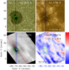 |
Fig. 1. Near-UV snapshots and CO large scan images on 2017 September 15 measured by the IRIS/SJI and GST/CYRA. The green contours represent the umbra–penumbra boundary. Two blue lines outline IRIS slits, and double red lines mark the first and last (13th) slits of CYRA. The two magenta plus signs (+) in panel c indicate the umbra–penumbra boundary positions at the first CYRA slit. The cyan asterisk (*) in panel c indicates a crossover point between the slits of IRIS and CYRA at the sunspot umbra. |
The sunspot was also measured by the CYRA, which is installed on the 1.6 m Goode Solar Telescope (GST) at BBSO (Cao et al. 2010; Cao 2012; Yang et al. 2020). Several CO molecular bands spread throughout the CYRA spectrum, and the fundamental rotation-vibration transition lines near 46 655 Å are unique because they are not obscured by the Earth’s atmosphere. Therefore, they are well-known diagnostics of the lower atmosphere of the Sun (e.g., Solanki et al. 1994; Cao et al. 2010; Penn 2014). During our observations GST/CYRA measured the sunspot between ∼16:50:14 UT and ∼17:15:14 UT, and it performed small quick 13-step raster scans with a step size of ∼0.4″, while the time cadence between two nearby raster scans is about 15 s. To co-align with other instruments, we also performed a large 400-step raster scan between around 18:14:13−18:18:23 UT with a step size of ∼0.2″. Figures 1c−d present the large scan images with the same FOV of around 66″ × 80″ in the line intensity and at the Doppler velocity of the CO 3-2 R14 line, respectively. Two oblique red lines indicate the first (solid) and 13th (dashed) slits of CYRA small raster scan, which are along a ∼29° angle to the solar north–south direction. Two magenta crosses indicate the crossover points between the first CYRA slit and the umbra–penumbra boundary. It can be seen that the slits of CYRA and IRIS overlap in one position (x ≈ −67″, y ≈ 23″) at the sunspot umbra, as shown by the cyan asterisk.
Figure 2a shows the solar infrared CO spectrum at ∼17:00:45 UT observed by GST/CYRA in its first slit, as indicated by the red solid line in Fig. 1. It has been pre-processed (see details in Appendix A). We note that the bright patch in the lower left corner of Fig. 2a are the hot pixels from the detector, which cannot be effectively corrected by the interpolation due to their patchy distribution. So we avoid using these regions in the following analysis. The overplotted curve in panel a is the CO line profile at the slit position of ∼38″, as indicated by a short cyan line on the left side. A number of absorption lines can be seen from the solar infrared spectrum, and eight obvious lines are identified and labeled with short magenta ticks, including seven CO molecular lines and a telluric line. In this paper, two CO molecular lines are used to study the sunspot oscillation: a strong line of CO 3-2 R14 and a weak line of CO 7-6 R67. Their formation height is around 500 km above the τ500 = 1 (z = 0), ranging from the photosphere through temperature minimum region to the low chromosphere. The weak line (CO 7-6 R67) is probing the lower solar layers, such as the photosphere. While the strong line (CO 3-2 R14) could vary from roughly 150 to 580 km above τ500 = 1, which probes the upper photosphere, the temperature minimum region, as well as the lower chromosphere (see also Uitenbroek 2000; Ayres et al. 2006).
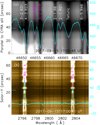 |
Fig. 2. Solar spectra in infrared (a) and NUV (b) wavebands at around ∼17:00 UT measured by CYRA and IRIS, respectively. The overplotted curves are the line spectra marked by a cyan line on the left side of each image. The main lines are labeled and indicated by magenta vertical ticks. |
Figure 2b presents the IRIS spectrum in NUV wavebands at around 17:00:41 UT in the second slit, as indicated by the blue solid line in Fig. 1. They have been pre-processed with the standard IRIS routines in SSW package (De Pontieu et al. 2014). The overplotted curves are the line profiles at the solar position nearby y ≈ 23″, as marked by a short cyan line on the left side of each panel. The double resonance lines of Mg II k & h are identified in panel b, and they are mostly formed in the chromosphere with a formation temperature of ∼104 K.
3. Data analysis and results
3.1. Spectroscopic diagnostics with two CO lines
GST/CYRA observed the sunspot in a quickly raster mode with 13 steps, and the scanned FOV was about 4.8″ × 80″, while the exposure time was ∼40 ms. The 13 slits of CYRA went through the sunspot umbra and penumbra in sequence, as shown in Fig. 1c. Figure 2 suggests that each CO molecular line near its center is clearly a Gaussian profile. Thus, we applied a single Gaussian fit (see Appendix B) to each line profile of CO molecule, i.e., CO 3-2 R14 and CO 7-6 R67 (see Uitenbroek et al. 1994; Uitenbroek 2000). Then their Doppler velocities and line intensities could be measured.
Figure 3 presents the time–distance images derived from the first slit of CYRA. That is, the y-axis is parallel to the slit direction between about 23″and 56″. We note that the short time disturbances near ∼17:04 UT and ∼17:10 UT correspond to the time when the image stabilization system does not work. It can be seen from panels a and b that the Doppler velocities of CO molecular lines are small, roughly ±0.5 km s−1. They all exhibit a pronounced signature of oscillations that change from redshifts to blueshifts, in particular at the umbra, i.e., between 35″ and 40″. The oscillation periods can be determined from the numbers of red patterns. Then a long period of roughly 5 min can be found in the CO 7-6 R67 line, while a short period of around 3 min can be discovered in the CO 3-2 R14 line at the sunspot umbra. We also find that the Doppler shift oscillations are similar at the penumbra, i.e., at the slit position near 30″ and 50″. However, there is not any apparent oscillation in the intensity image (c) of CO 3-2 R14 line at the sunspot. Two magenta lines mark the umbra–penumbra boundaries, which are indicated by the two plus signs (+) in Fig. 1c. Here we do not show the line intensity of CO 7-6 R67 line since it does not exhibit the pronounced oscillation feature.
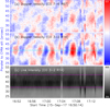 |
Fig. 3. Time–distance images along the first CYRA slit (red solid line in Fig. 1) of Doppler velocity and intensity in CO 3-2 R14 and CO 7-6 R67 lines. The y-axis is parallel to the slits of CYRA. A horizontal cyan line in panel b outline the umbral position to perform the wavelet analysis in Figs. 6 and 7. Two magenta lines outline the umbra–penumbra boundary. |
To spatially resolved the sunspot oscillation, we then plot the time–distance images along the CYRA scanned direction, as shown in Fig. 4. In other words, the y-axis is perpendicular to the slits of CYRA with a length of around 4.8″, and the first slit corresponds to bottom position, while the 13th slit is in the upper location. Their Doppler velocities are both characterized by a number of vertical slashes that change from redshift to blueshift, including the strong line of CO 3-2 R14 and the weak CO 7-6 R67 line. These repeating dynamical behaviors can be considered sunspot oscillations. It seems that the CO 3-2 R14 and CO 7-6 R67 lines both show the same period of 5 min at most regions. In the bottom region (*) of panel b, there seem to be more red patterns than in the other regions, suggesting a short period at the umbra. All these observational results agree with the previous findings (see Fig. 3).
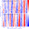 |
Fig. 4. Time–distance images of Doppler velocity in CO 3-2 R14 and CO 7-6 R67 lines. The y-axis is perpendicular to the slits of CYRA. The cyan asterisks (*) symbol indicates the start point on the y-axis, which is same as in Fig. 1c. |
3.2. Spectroscopic observations in the Mg II k line
IRIS measured the sunspot in two-step raster mode between 16:40:15 UT and 18:01:59 UT. The spectrograph aboard IRIS covered a small FOV of around 2″ × 119″, with an exposure time of ∼8 s. Luckily, the slits of IRIS nearly crossed the sunspot center, and the second slit (blue solid line in Fig. 1) was crossed by the first slit of CYRA (red solid line in Fig. 1) at the sunspot umbra, (cyan asterisk in Fig. 1g). So, the IRIS spectra from its second slit were used to investigate the sunspot oscillation. The double resonance lines of Mg II k \AMP h are usually optically thick in solar spectra, and their line profiles often exhibit central reversals at line cores (Leenaarts et al. 2013; Cheng et al. 2015). However, the Mg II k & h lines at sunspots do not appear to be the prominent central reversals of line cores (see Tian et al. 2014; Zhang et al. 2017). Figure 2b shows the line profiles of Mg II k & h lines at sunspot umbra, and their line cores are not central reversals, but they are also non-Gaussian profiles. Therefore, the moment analysis method but not the single Gaussian fit is applied to estimate their Doppler velocities, line widths, and intensities (see detail in Li et al. 2017).
Figure 5 presents the time–distance images of Doppler velocity (a), line intensity (b), and line width (c) in the Mg II k line. Here, the y-axis is parallel to the slits of IRIS (blue lines) with a length of ∼33″ in the approximate range of 6″ − 39″ along the solar-Y direction. The Doppler velocities of Mg II k line at the umbra near y ∼ 23″ exhibit pronounced oscillations with a quasi-period of around 3 min. They are characterized by a group of repeating oblique streaks, which changing from redshift to blueshift. The oblique streaks suggest that they are propagating and eventually become invisible at the umbra–penumbra boundary. The line intensity and width show the same oscillation behaviors. For example, the 3 min oscillation is identified as the repeating oblique slashes at the sunspot umbra, which also exhibit a propagation movement and gradually disappear when they reach the outer umbral boundary. Finally, we do not find any clear signature of oscillations at the penumbra, such as at the positions of around y ∼ 10″ and y ∼ 35″.
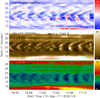 |
Fig. 5. Time–distance images along the second slit of IRIS (blue solid line in Fig. 1) of Doppler velocity, line width, and intensity in Mg II k. The horizontal cyan line in panel a gives the umbral position, used to perform the wavelet analysis in Fig. 8. |
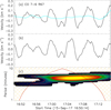 |
Fig. 6. Wavelet analysis result in the CO 7-6 R67 line at the sunspot umbra. Panel a: Doppler velocity (black) and its trend (cyan). Panel b: detrended velocity. Panel c: wavelet power spectrum. The red line indicates a significance level of 99%. |
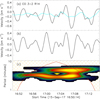 |
Fig. 7. Wavelet analysis result in the CO 3-2 R14 line at the same umbral position. Panel a: Doppler velocity (black) and its trend (cyan). Panel b: detrended velocity. Panel c: wavelet power spectrum. The red line indicates a significance level of 99%. |
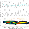 |
Fig. 8. Wavelet analysis result in the Mg II k line at the same umbral position. Panel a: Doppler velocity (black) and its trend (cyan). Panel b: detrended velocity. Panel c: wavelet power spectrum. The red line indicates a significance level of 99%. |
3.3. Wavelet analysis
To look closely at the periods of the sunspot oscillation at the umbra, we then performed wavelet analysis (e.g., Torrence & Compo 1998; Chae et al. 2017; Cho et al. 2019) on the detrended time series of Doppler velocities at the sunspot umbra, as indicated by the cyan line in Figs. 3 and 5. It should be noted that it is the same position at the sunspot umbra, which is indicated with the cyan asterisk in Fig. 1c. The detrended time series are used here because we thereby enhance the periods, for example 3 or 5 min. The discussion and application of this method can be found in previous works (Gruber et al. 2011; Kupriyanova et al. 2013; Li et al. 2020).
Figure 6 presents the wavelet analysis result of the Doppler velocity in CO 7-6 R67 line. Panel a shows the time series between ∼16:50:14 UT and 17:15:14 UT of the Doppler velocity at the sunspot umbra, as indicated with the cyan asterisk in Fig. 1c. The Doppler velocity (black) in the CO 7-6 R67 line is very low, with a peak value of roughly 0.2 km s−1. Then the trend Doppler velocity is overplotted with cyan line, which is a four-minute running average. It can be seen that the trend velocity is close to zero. Panel b displays the detrended velocity after subtracting the four-minute running average (e.g., Wang et al. 2009; Li et al. 2018), which exhibits five pronounced peaks within a duration of 25 minutes, suggesting a 5 min periodicity. The 5 min periodicity is confirmed by the wavelet power spectrum shown in panel c. It clearly shows a period of 5 min above the confidence level of 99% (red contour).
Figure 7 shows the wavelet analysis result of the Doppler velocity in CO 3-2 R14 line during the same time interval, i.e., from ∼16:50:14 UT to ∼17:15:14 UT. The Doppler velocity here is a little higher than that of CO 7-6 R67 line, i.e., the peak value can be reach to ∼0.5 km s−1, as shown by the black curve in panel a. The detrended velocity also appears as several pronounced peaks, but there are also some small peaks, as seen in panel b. Thus, it is hard to determine a single period through the peaks. The period can be identified in the wavelet power spectrum, as given in panel c. It exhibits two prominent periods, one is a 3 min periodicity and can be detected almost at the observed time, the other is 5 min periodicity that only appears after ∼17:00 UT.
The similar wavelet analysis result of the Doppler velocity in Mg II k line is shown in Fig. 8. At the same umbra position, The Doppler velocities are much higher that those in the CO molecular lines, which can be as high as ∼8 km s−1, as shown in panel a. The wavelet power spectrum exhibits a dominant period of around 3 min, which agrees with the 3 min periodicity derived from the CO 3-2 R14 line.
3.4. Cross-correlation analysis
To analyze the phase relation between different atmospheric levels, for example two CO molecular lines and Mg II k line, a cross-correlation analysis (e.g., Tian et al. 2014; Krishna Prasad et al. 2015; Su et al. 2016) is applied for the detrended time series to investigate their time delays, as shown in Fig. 9. A maximum correlation coefficient of ∼0.77 between the strong CO 3-2 R14 line and the weak CO 7-6 R67 line is found at the time lag of around -0.3 minute, implying a short time delay between them; in other words, the formation height of the strong CO 3-2 R14 line is a little higher than that of the weak CO 7-6 R67 line, which is similar to previous observations (Uitenbroek 2000; Ayres 2002). On the other hand, a maximum correlation coefficient of ∼0.52 between CO 3-2 R14 and Mg II k lines is discovered at the time lag of about 2 min, suggesting a long time delay between them. It should be noted that the time delay between CO 3-2 R14 and Mg II k lines here suggests that the 3 min oscillation at sunspot umbra is a propagating wave, which agrees with previous observations about the propagating slow wave in sunspots (see Khomenko & Collados 2015; Krishna Prasad et al. 2015; Wang et al. 2018).
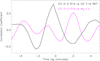 |
Fig. 9. Correlation coefficients between two parameters as a function of the time lag: the Doppler velocities between two CO molecular lines (black), and the strong CO 3-2 R14 and Mg II k lines (magenta). |
4. Conclusion and discussion
Using the spectroscopic observations in solar infrared and NUV bands measured by the GST/CYRA and the IRIS, we investigated the sunspot oscillation in Doppler velocities of two CO molecular lines and the Mg II k line. The weak line of CO 7-6 R67 exhibits the 5 min oscillation at the sunspot umbra (Fig. 6). However, the strong CO 3-2 R14 line shows double periods at the sunspot umbra (Fig. 7) of nearly 5 min and roughly 3 min. The double oscillation periods could be due to the fact that the strong CO 3-2 R14 line contains two-layer radiation on the Sun, i.e., the upper photosphere and temperature minimum region (Uitenbroek 2000; Ayres et al. 2006). The line profiles of Mg II k lines also show the typical 3 min oscillation at the sunspot umbra, as shown in Fig. 8. On the other hand, an oscillation period of around 5 min can be found in the two CO molecular lines at the sunspot penumbra, but it is not detected in the Mg II k line. Therefore, only the sunspot oscillation at the umbra is studied in detail.
An interesting aspect is that the sunspot oscillation can be spatially resolved in the Doppler shifts, i.e., they can be discovered in three directions above sunspot at the solar atmosphere, for instance the directions that are perpendicular and parallel to the CYRA slit, and also parallel to the IRIS slit. This is different from previous spatial distributions of sunspot oscillations observed in intensity images (e.g., Yuan et al. 2014; Wang et al. 2020; Yurchyshyn et al. 2020). Figures 3 and 4 demonstrate that the sunspot oscillations at the umbra and penumbra can appear in the directions perpendicular and parallel to the CYRA slits, including the long period of nearly 5 min and the short period of around 3 min. Meanwhile, we demonstrated that the CYRA slits show a roll angle of ∼29° with the slits of IRIS, as can be seen in Fig. 1c. The 3 min oscillation at the umbra (around y ∼ 20″) can also be found parallel to the slits of IRIS, as can be seen in Fig. 5. Therefore, our observational results suggest that the sunspot oscillation (particularly the umbral oscillation) can be found in an arbitrary direction, which is similar to the running umbral waves (Alissandrakis et al. 1998; Kobanov & Makarchik 2004). All these observational results imply that they can be considered trans-sunspot waves (Tziotziou et al. 2006; Chae et al. 2017). Finally, the sunspot oscillation could be detected in two perpendicular directions, which is benefited from the fast scan of the CYRA with 13 steps.
We wanted to discuss the observed periods at sunspot. A period of nearly five minutes can be detected in Doppler velocities of CO 3-2 R14 and 7-6 R67 lines, which is consistent with previous findings in white light images or continuum spectrum (Beckers & Schultz 1972; Lites 1988; Nagashima et al. 2007; Yuan et al. 2014; Su et al. 2016), and might be considered the solar p-mode waves in the photosphere (Thomas 1985; Bogdan 2000; Solanki 2003). While a period of roughly three minutes is found in the Doppler velocities of the CO 3-2 R14 and Mg II k lines, which agrees closely with the previous observational results in UV–infrared lines or images at the sunspot umbra (e.g., Solanki et al. 1996; Bogdan 2000; Fludra 2001; Maltby et al. 2001; Centeno et al. 2008; Tian et al. 2014; Khomenko & Collados 2015; Yang et al. 2017). They are explained as the resonant modes of sunspot oscillations (Uexkuell et al. 1983; Thomas 1984; Gurman 1987; Khomenko & Collados 2015). On the other hand, the CO 3-2 R14 line is believed to provide the information in the upper photosphere or the temperature minimum region (Uitenbroek 2000; Ayres 2002; Ayres et al. 2006). Moreover, a time delay of about two minutes is measured between the CO 3-2 R14 and Mg II k lines, as shown in Fig. 9. So, the three-minute oscillation at the sunspot umbra could come from the upper photosphere or the temperature minimum region and then propagate to the chromosphere, supporting the interpretation that propagating waves above the sunspots originate from the lower solar atmosphere (De Moortel et al. 2002; O’Shea et al. 2002; Brynildsen et al. 2004; Khomenko & Collados 2015; Krishna Prasad et al. 2015). In other words, the three-minute oscillation can be regarded as the upwardly propagating slow magnetoacoustic waves (e.g., Su et al. 2016; Chae et al. 2019; Cho & Chae 2020; Feng et al. 2020b). Finally, Chae et al. (2017) found that the three-minute oscillation in the light bridge or umbral dots of a sunspot originates from the photosphere (see aslo Cho et al. 2019), which is consistent with our results and further suggests that the CYRA data is reliable.
Acknowledgments
We acknowledge the anonymous referee for his/her valuable comments. BBSO operation is supported by US NSF AGS 1821294 grant and NJIT. GST operation is partly supported by the Korea Astronomy and Space Science Institute, the Seoul National University, and the Key Laboratory of Solar Activities of Chinese Academy of Sciences (CAS) and the Operation, Maintenance and Upgrading Fund of CAS for Astronomical Telescopes and Facility Instruments. We also thank the teams of IRIS for their open data use policy. This study is supported by NSFC under grants 11973092, 11427901, 11773038, 11873062, 11790300, 11790302, 11729301, 11873095, 12073081, the Youth Fund of Jiangsu No. BK20171108, as well as National Natural Science Foundation of China (U1731241), the Strategic Priority Research Program on Space Science, CAS, Grant No. XDA15052200 and XDA15320301. D. Li is supported by CAS Key Laboratory of Solar Activity (KLSA202003) and the Specialized Research Fund for State Key Laboratories. The Laboratory No. 2010DP173032.
References
- Alissandrakis, C. E., Tsiropoula, G., & Mein, P. 1998, ASP Conf. Ser., 155, 49 [NASA ADS] [Google Scholar]
- Ayres, T. R. 2002, ApJ, 575, 1104 [NASA ADS] [CrossRef] [Google Scholar]
- Ayres, T. R., & Brault, J. W. 1990, ApJ, 363, 705 [NASA ADS] [CrossRef] [Google Scholar]
- Ayres, T. R., & Wiedemann, G. R. 1989, ApJ, 338, 1033 [NASA ADS] [CrossRef] [Google Scholar]
- Ayres, T. R., Plymate, C., & Keller, C. U. 2006, ApJS, 165, 618 [NASA ADS] [CrossRef] [Google Scholar]
- Beckers, J. M., & Schultz, R. B. 1972, Sol. Phys., 27, 61 [NASA ADS] [CrossRef] [Google Scholar]
- Bellot Rubio, L. R., Collados, M., Ruiz Cobo, B., & Rodríguez Hidalgo, I. 2000, ApJ, 534, 989 [NASA ADS] [CrossRef] [Google Scholar]
- Bloomfield, D. S., Lagg, A., & Solanki, S. K. 2007, ApJ, 671, 1005 [NASA ADS] [CrossRef] [Google Scholar]
- Bogdan, T. J. 2000, Sol. Phys., 192, 373 [NASA ADS] [CrossRef] [Google Scholar]
- Borrero, J. M., & Ichimoto, K. 2011, Liv. Rev. Sol. Phys., 8, 4 [Google Scholar]
- Brynildsen, N., Maltby, P., Foley, C. R., Fredvik, T., & Kjeldseth-Moe, O. 2004, Sol. Phys., 221, 237 [NASA ADS] [CrossRef] [Google Scholar]
- Cao, W. 2012, IAU Spec. Session, 6(E2), 02 [Google Scholar]
- Cao, W., Gorceix, N., Coulter, R., et al. 2010, Astron. Nachr., 331, 636 [NASA ADS] [CrossRef] [Google Scholar]
- Centeno, R., Trujillo Bueno, J., Uitenbroek, H., & Collados, M. 2008, ApJ, 677, 742 [NASA ADS] [CrossRef] [Google Scholar]
- Chae, J., & Goode, P. R. 2015, ApJ, 808, 118 [NASA ADS] [CrossRef] [Google Scholar]
- Chae, J., Lee, J., Cho, K., et al. 2017, ApJ, 836, 18 [NASA ADS] [CrossRef] [Google Scholar]
- Chae, J., Kang, J., & Litvinenko, Y. E. 2019, ApJ, 883, 72 [CrossRef] [Google Scholar]
- Cheng, X., Ding, M. D., & Fang, C. 2015, ApJ, 804, 82 [NASA ADS] [CrossRef] [Google Scholar]
- Cho, K., & Chae, J. 2020, ApJ, 892, L31 [CrossRef] [Google Scholar]
- Cho, K., Chae, J., & Lim, E.-K. 2019, ApJ, 879, 67 [CrossRef] [Google Scholar]
- Cram, L. E., & Thomas, J. H. 1981, Nature, 293, 101 [CrossRef] [Google Scholar]
- De Moortel, I., Ireland, J., Hood, A. W., & Walsh, R. W. 2002, A&A, 387, L13 [NASA ADS] [CrossRef] [EDP Sciences] [Google Scholar]
- De Pontieu, B., Title, A. M., Lemen, J. R., et al. 2014, Sol. Phys., 289, 2733 [NASA ADS] [CrossRef] [Google Scholar]
- Feng, S., Yu, L., Yang, Y.-F., et al. 2014, Res. Astron. Astrophys., 14, 1001 [CrossRef] [Google Scholar]
- Feng, S., Miao, Y., Yuan, D., et al. 2020a, ApJ, 893, L2 [CrossRef] [Google Scholar]
- Feng, S., Deng, Z., Yuan, D., et al. 2020b, Res. Astron. Astrophys., 20, 117 [CrossRef] [Google Scholar]
- Fludra, A. 2001, A&A, 368, 639 [NASA ADS] [CrossRef] [EDP Sciences] [Google Scholar]
- Goorvitch, D. 1994, ApJS, 95, 535 [NASA ADS] [CrossRef] [Google Scholar]
- Gruber, D., Lachowicz, P., Bissaldi, E., et al. 2011, A&A, 533, A61 [NASA ADS] [CrossRef] [EDP Sciences] [Google Scholar]
- Gurman, J. B. 1987, Sol. Phys., 108, 61 [NASA ADS] [CrossRef] [Google Scholar]
- Howard, R., Tanenbaum, A. S., & Wilcox, J. M. 1968, Sol. Phys., 4, 286 [CrossRef] [Google Scholar]
- Jess, D. B., Reznikova, V. E., Ryans, R. S. I., et al. 2016, Nat. Phys., 12, 179 [NASA ADS] [CrossRef] [Google Scholar]
- Khomenko, E., & Cally, P. S. 2012, ApJ, 746, 68 [NASA ADS] [CrossRef] [Google Scholar]
- Khomenko, E., & Collados, M. 2015, Liv. Rev. Sol. Phys., 12, 6 [CrossRef] [Google Scholar]
- Kobanov, N. I., & Makarchik, D. V. 2004, A&A, 424, 671 [NASA ADS] [CrossRef] [EDP Sciences] [Google Scholar]
- Krishna Prasad, S., Jess, D. B., & Khomenko, E. 2015, ApJ, 812, L15 [NASA ADS] [CrossRef] [Google Scholar]
- Kupriyanova, E. G., Melnikov, V. F., & Shibasaki, K. 2013, Sol. Phys., 284, 559 [NASA ADS] [CrossRef] [Google Scholar]
- Lagg, A., Solanki, S. K., van Noort, M., & Danilovic, S. 2014, A&A, 568, A60 [NASA ADS] [CrossRef] [EDP Sciences] [Google Scholar]
- Leenaarts, J., Pereira, T. M. D., Carlsson, M., Uitenbroek, H., & De Pontieu, B. 2013, ApJ, 772, 89 [NASA ADS] [CrossRef] [Google Scholar]
- Li, Y., Kelly, M., Ding, M. D., et al. 2017, ApJ, 848, 118 [NASA ADS] [CrossRef] [Google Scholar]
- Li, D., Yuan, D., Su, Y. N., et al. 2018, A&A, 617, A86 [NASA ADS] [CrossRef] [EDP Sciences] [Google Scholar]
- Li, D., Kolotkov, D. Y., Nakariakov, V. M., et al. 2020, ApJ, 888, 53 [Google Scholar]
- Lites, B. W. 1986, ApJ, 301, 1005 [NASA ADS] [CrossRef] [Google Scholar]
- Lites, B. W. 1988, ApJ, 334, 1054 [NASA ADS] [CrossRef] [Google Scholar]
- Löhner-Böttcher, J., Schmidt, W., Schlichenmaier, R., et al. 2018, A&A, 617, A19 [NASA ADS] [CrossRef] [EDP Sciences] [Google Scholar]
- Maltby, P., Brynildsen, N., Kjeldseth-Moe, O., & Wilhelm, K. 2001, A&A, 373, L1 [NASA ADS] [CrossRef] [EDP Sciences] [Google Scholar]
- Maunder, E. W. 1904, MNRAS, 64, 747 [NASA ADS] [Google Scholar]
- Nagashima, K., Sekii, T., Kosovichev, A. G., et al. 2007, PASJ, 59, S631 [NASA ADS] [CrossRef] [Google Scholar]
- Noyes, R. W., & Hall, D. N. B. 1972, ApJ, 176, L89 [NASA ADS] [CrossRef] [Google Scholar]
- O’Shea, E., Muglach, K., & Fleck, B. 2002, A&A, 387, 642 [NASA ADS] [CrossRef] [EDP Sciences] [Google Scholar]
- Penn, M. J. 2014, Liv. Rev. Sol. Phys., 11, 2 [Google Scholar]
- Penn, M. J., Schad, T., & Cox, E. 2011, ApJ, 734, 47 [CrossRef] [Google Scholar]
- Phillis, G. L. 1975, Sol. Phys., 41, 71 [CrossRef] [Google Scholar]
- Rimmele, T. R. 1997, ApJ, 490, 458 [NASA ADS] [CrossRef] [Google Scholar]
- Rouppe van der Voort, L. H. M., Rutten, R. J., Sütterlin, P., Sloover, P. J., & Krijger, J. M. 2003, A&A, 403, 277 [NASA ADS] [CrossRef] [EDP Sciences] [Google Scholar]
- Scheuer, M. A., & Thomas, J. H. 1981, Sol. Phys., 71, 21 [NASA ADS] [CrossRef] [Google Scholar]
- Schüssler, M., & Vögler, A. 2006, ApJ, 641, L73 [NASA ADS] [CrossRef] [Google Scholar]
- Sobotka, M., Bonet, J. A., & Vazquez, M. 1994, ApJ, 426, 404 [NASA ADS] [CrossRef] [Google Scholar]
- Solanki, S. K. 2003, A&A Rev., 11, 153 [NASA ADS] [CrossRef] [Google Scholar]
- Solanki, S. K., Livingston, W., & Ayres, T. 1994, Science, 263, 64 [NASA ADS] [CrossRef] [PubMed] [Google Scholar]
- Solanki, S. K., Livingston, W., Muglach, K., & Wallace, L. 1996, A&A, 315, 303 [NASA ADS] [Google Scholar]
- Soltau, D., Schroeter, E. H., & Woehl, H. 1976, A&A, 50, 367 [NASA ADS] [Google Scholar]
- Su, J. T., Ji, K. F., Cao, W., et al. 2016, ApJ, 817, 117 [NASA ADS] [CrossRef] [Google Scholar]
- Thomas, J. H. 1984, A&A, 135, 188 [NASA ADS] [Google Scholar]
- Thomas, J. H. 1985, Aust. J. Phys., 38, 811 [NASA ADS] [CrossRef] [Google Scholar]
- Tian, H., DeLuca, E., Reeves, K. K., et al. 2014, ApJ, 786, 137 [NASA ADS] [CrossRef] [Google Scholar]
- Torrence, C., & Compo, G. P. 1998, Bull. Am. Meteorol. Soc., 79, 61 [Google Scholar]
- Toriumi, S., Katsukawa, Y., & Cheung, M. C. M. 2015, ApJ, 811, 137 [NASA ADS] [CrossRef] [Google Scholar]
- Tziotziou, K., Tsiropoula, G., Mein, N., & Mein, P. 2006, A&A, 456, 689 [NASA ADS] [CrossRef] [EDP Sciences] [Google Scholar]
- Uexkuell, M. V., Kneer, F., & Mattig, W. 1983, A&A, 123, 263 [Google Scholar]
- Uitenbroek, H. 2000, ApJ, 531, 571 [NASA ADS] [CrossRef] [Google Scholar]
- Uitenbroek, H., Noyes, R. W., & Rabin, D. 1994, ApJ, 432, L67 [NASA ADS] [CrossRef] [Google Scholar]
- Wang, T. J., Ofman, L., & Davila, J. M. 2009, ApJ, 696, 1448 [NASA ADS] [CrossRef] [Google Scholar]
- Wang, F., Deng, H., Li, B., et al. 2018, ApJ, 856, L16 [NASA ADS] [CrossRef] [Google Scholar]
- Wang, Z.-K., Feng, S., Deng, L.-H., et al. 2020, Res. Astron. Astrophys., 20, 006 [CrossRef] [Google Scholar]
- Wittmann, A. 1969, Sol. Phys., 7, 366 [NASA ADS] [CrossRef] [Google Scholar]
- Wittmann, A. D., & Xu, Z. T. 1987, A&AS, 70, 83 [NASA ADS] [Google Scholar]
- Wolf, R. 1861, MNRAS, 21, 77 [NASA ADS] [Google Scholar]
- Yang, S., Zhang, J., Erdélyi, R., et al. 2017, ApJ, 843, L15 [CrossRef] [Google Scholar]
- Yang, X., Cao, W. D., & Gorceix, N. 2020, ArXiv e-prints [arXiv:2008.11320] [Google Scholar]
- Yau, K. K. C., & Stephenson, F. R. 1988, QJRAS, 29, 175 [Google Scholar]
- Yuan, D. 2015, Res. Astron. Astrophys., 15, 1449 [CrossRef] [Google Scholar]
- Yuan, D., Sych, R., Reznikova, V. E., & Nakariakov, V. M. 2014, A&A, 561, A19 [NASA ADS] [CrossRef] [EDP Sciences] [Google Scholar]
- Yurchyshyn, V., Kilcik, A., Şahin, S., et al. 2020, ApJ, 896, 150 [CrossRef] [Google Scholar]
- Zhang, J., Tian, H., He, J., & Wang, L. 2017, ApJ, 838, 2 [NASA ADS] [CrossRef] [Google Scholar]
- Zhugzhda, Y., & Sych, R. 2018, Res. Astron. Astrophys., 18, 105 [CrossRef] [Google Scholar]
Appendix A: CYRA instrument and data calibration
CYRA is the first fully cold cryogenic solar spectrograph, and the detector currently used by CYRA is a commercial detector rather than a scientific one (Cao 2012). All CYRA components (e.g., slit, grating, collimator/imager, order sorting filter, and detector) are placed in a dual-layer cryostat working at very low temperature, i.e., ∼77 K for the outer case and ∼30 K for the inner case. Thus, the thermal background emission is tremendously minimized (Cao et al. 2010; Yang et al. 2020). It works at the wavelength region in the range 10 000−50 000 Å, and the maximum frame rate of the 2 k × 2 k detector is 76 Hz.
The raw images observed by the CYRA have been pre-processed in the following way:
-
1.
The dark images obtained by exposing with the main cover of GST closed are subtracted.
-
2.
The dark subtracted images are corrected for flat fields, which are performed by averaging hundreds of frames taken by randomly moving the telescope near the solar disk center. The spatially averaged spectrum along the slit is also removed during the calculation of flat fields.
-
3.
The values of bad pixels from the dark-subtracted and flat-fielding images are replaced with a linear interpolation from neighboring pixels.
-
4.
The spectrum is corrected for the slant and distortion in both slit and dispersion directions. Then the wavelength jitter or drift are done according to a telluric line nearby the CO lines. After the above-mentioned calibration, there are still some residual distinct stripe patterns, and the derived physical parameters vary along the slit, which are further obtained and corrected by averaging the scanned quiet regions in the 400-step raster scanned image and the time sequences of the derived physical parameters in the 13-step raster scans.
-
5.
The Doppler velocity calibration is done based on the phenomenon that the average value of Doppler velocities in the sunspot umbra is almost zero (e.g., Löhner-Böttcher et al. 2018). The velocity calibration for the data from the 13-step raster is done with the assumption that the averaged value in the time sequences is near zero.
Appendix B: Gaussian fit to the CO line
In this study we presented the single Gaussian fitting result and its original observational line profile near the line center of both the CO 7-6 R67 and the CO 3-2 R14 lines, as shown in Fig. B.1. It can be found that the single Gaussian fit agrees well with its corresponding original profile. Moreover, Uitenbroek (2000) also used the single Gaussian fit to derive these parameters for CO lines. Penn et al. (2011) compared the Gaussian fitting result with Voigt fitting method and no systematic differences were seen in the derived line center wavelength. On the basis of the above considerations, we finally used the single Gaussian fits to the CO lines profiles.
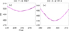 |
Fig. B.1. Example of the CO weak (a) and strong (b) line fitting results (magenta) with the single Gaussian fit method. The black line represents the corresponding observational profile measured by CYRA. |
All Tables
All Figures
|
Fig. 1. Near-UV snapshots and CO large scan images on 2017 September 15 measured by the IRIS/SJI and GST/CYRA. The green contours represent the umbra–penumbra boundary. Two blue lines outline IRIS slits, and double red lines mark the first and last (13th) slits of CYRA. The two magenta plus signs (+) in panel c indicate the umbra–penumbra boundary positions at the first CYRA slit. The cyan asterisk (*) in panel c indicates a crossover point between the slits of IRIS and CYRA at the sunspot umbra. |
| In the text | |
|
Fig. 2. Solar spectra in infrared (a) and NUV (b) wavebands at around ∼17:00 UT measured by CYRA and IRIS, respectively. The overplotted curves are the line spectra marked by a cyan line on the left side of each image. The main lines are labeled and indicated by magenta vertical ticks. |
| In the text | |
|
Fig. 3. Time–distance images along the first CYRA slit (red solid line in Fig. 1) of Doppler velocity and intensity in CO 3-2 R14 and CO 7-6 R67 lines. The y-axis is parallel to the slits of CYRA. A horizontal cyan line in panel b outline the umbral position to perform the wavelet analysis in Figs. 6 and 7. Two magenta lines outline the umbra–penumbra boundary. |
| In the text | |
|
Fig. 4. Time–distance images of Doppler velocity in CO 3-2 R14 and CO 7-6 R67 lines. The y-axis is perpendicular to the slits of CYRA. The cyan asterisks (*) symbol indicates the start point on the y-axis, which is same as in Fig. 1c. |
| In the text | |
|
Fig. 5. Time–distance images along the second slit of IRIS (blue solid line in Fig. 1) of Doppler velocity, line width, and intensity in Mg II k. The horizontal cyan line in panel a gives the umbral position, used to perform the wavelet analysis in Fig. 8. |
| In the text | |
|
Fig. 6. Wavelet analysis result in the CO 7-6 R67 line at the sunspot umbra. Panel a: Doppler velocity (black) and its trend (cyan). Panel b: detrended velocity. Panel c: wavelet power spectrum. The red line indicates a significance level of 99%. |
| In the text | |
|
Fig. 7. Wavelet analysis result in the CO 3-2 R14 line at the same umbral position. Panel a: Doppler velocity (black) and its trend (cyan). Panel b: detrended velocity. Panel c: wavelet power spectrum. The red line indicates a significance level of 99%. |
| In the text | |
|
Fig. 8. Wavelet analysis result in the Mg II k line at the same umbral position. Panel a: Doppler velocity (black) and its trend (cyan). Panel b: detrended velocity. Panel c: wavelet power spectrum. The red line indicates a significance level of 99%. |
| In the text | |
|
Fig. 9. Correlation coefficients between two parameters as a function of the time lag: the Doppler velocities between two CO molecular lines (black), and the strong CO 3-2 R14 and Mg II k lines (magenta). |
| In the text | |
|
Fig. B.1. Example of the CO weak (a) and strong (b) line fitting results (magenta) with the single Gaussian fit method. The black line represents the corresponding observational profile measured by CYRA. |
| In the text | |
Current usage metrics show cumulative count of Article Views (full-text article views including HTML views, PDF and ePub downloads, according to the available data) and Abstracts Views on Vision4Press platform.
Data correspond to usage on the plateform after 2015. The current usage metrics is available 48-96 hours after online publication and is updated daily on week days.
Initial download of the metrics may take a while.