| Issue |
A&A
Volume 698, June 2025
|
|
|---|---|---|
| Article Number | A259 | |
| Number of page(s) | 7 | |
| Section | The Sun and the Heliosphere | |
| DOI | https://doi.org/10.1051/0004-6361/202555021 | |
| Published online | 19 June 2025 | |
Doppler velocity oscillations in an Hα network rosette
1
Astronomy Program, Department of Physics and Astronomy, Seoul National University, Gwanak-gu, Seoul, 08826
Republic of Korea
2
Astronomy Research Center, Seoul National University, Gwanak-gu, Seoul, 08826
Republic of Korea
3
Korea Astronomy and Space Science Institute, Daedeokdae-ro, Yuseong-gu, Daejeon, 34055
Republic of Korea
4
Max-Planck Institute for Solar System Research, Justus-von-Liebig-Weg 3, 37077
Göttingen, Germany
5
Space Research and Technology Institute, Bulgarian Academy of Sciences, Acad. Georgy Bonchev Str., Bl. 1, 1113
Sofia, Bulgaria
⋆ Corresponding author: This email address is being protected from spambots. You need JavaScript enabled to view it.
Received:
3
April
2025
Accepted:
13
May
2025
Abstract
Magnetic flux tubes such as sunspots play the role of channels through which magnetohydrodynamic waves carry mechanical energy from the solar interior to the atmosphere. We investigate the spatial distribution of Doppler velocity oscillations in the chromospheric network rosette, a supposed quiet Sun miniature of a sunspot, by analyzing Hα line spectral data taken with the Fast Imaging Solar Spectrograph of the Goode Solar Telescope. The rosette consists of two regions: a central region displaying Hα emission and a fibril region displaying Hα absorption. We have categorized the observed velocity oscillations into three groups depending on location and period. Group I oscillations with periods from 3 to 6 min occur in the central region, group II oscillations with periods from 6 to 20 min in the inner parts of the fibril region, and group III oscillations with periods shorter than 3 min in the outermost parts of the fibril region. We discuss the probable physical origin of oscillations of each group. Our results suggest that the rosette is similar to a sunspot in morphology and oscillation properties, but there exist differences as well.
Key words: magnetohydrodynamics (MHD) / Sun: atmosphere / Sun: chromosphere / Sun: oscillations
© The Authors 2025
 Open Access article, published by EDP Sciences, under the terms of the Creative Commons Attribution License (https://creativecommons.org/licenses/by/4.0), which permits unrestricted use, distribution, and reproduction in any medium, provided the original work is properly cited.
This article is published in open access under the Subscribe to Open model. This email address is being protected from spambots. You need JavaScript enabled to view it. to support open access publication.
1. Introduction
Magnetic flux tubes are the basic building blocks of solar magnetic fields. They play the role of channels through which magnetohydrodynamic (MHD) waves transport mechanical energy from the solar interior to the atmosphere. Photospheric magnetic fields mainly exist in bright filigree points of network regions and faculae (Dunn & Zirker 1973; Mehltretter 1974) or in sunspots of active regions. A bright filigree point contrasts with a sunspot not only in brightness, but also in diameter. It corresponds to a thin flux tube for which the diameter is smaller than the pressure scale height, whereas a sunspot corresponds to a thick flux tube for which the diameter is much bigger than the pressure scale height.
A rosette is a rose-shaped Hα feature that often appears in network regions (e.g., Tsiropoula et al. 2012). An example is given in Figure 1. It comprises a central region that is usually bright in Hα core and contains chromospheric bright points seen in the Hα far wings, and the surrounding fibril region containing dark fibrils. The chromospheric bright points are mostly co-spatial with bright filigree points in the photosphere. A rosette appears as an organized structure in the chromosphere at a scale much larger than the diameters of individual bright points, so its magnetic structure in the chromosphere and corona may be regarded as a sunspot-like thick flux tube that is formed by the merging of a cluster of thinner flux tubes in the photosphere. If this is the case, it is expected that a systematic pattern of chromospheric oscillations and waves, as is observed in a sunspot, may be observable in a rosette as well. This expectation motivated the present work.
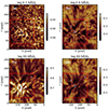 |
Fig. 1. Monochromatic images constructed from the reference raster (17:28:37 UT) at several wavelengths. The field of view is 32″ by 41″ and the spatial sampling size of 0.16″ is in each direction. The red squares indicate the region of interest, and the symbols mark the four positions selected to illustrate the time variation in the Doppler velocity and its wavelet analysis. |
A sunspot constantly hosts slow-body MHD waves of significant power. These sunspot waves have been observationally known as umbral oscillations (Giovanelli 1972), umbral flashes (Beckers & Tallant 1969), and running penumbral waves (Zirin & Stein 1972). Sunspot waves display systematic patterns. The period (typically 3 min) of the predominant oscillation in the umbra of a sunspot is known to be comparable to the acoustic cutoff period that is determined by the minimum temperature of the atmosphere (e.g., Chae & Litvinenko 2018; Chae et al. 2019). The predominant period increases with the distance from the sunspot center, resulting in longer periods (typically 5 min) of oscillations in the penumbra (Maurya et al. 2013; Jess et al. 2013; Sych et al. 2024) and even longer periods (> 10 min) in the super-penumbra (Chae et al. 2014). The presence of long-period oscillations as well as 3-min oscillations and 5-min oscillations in sunspots was also indicated from the radioheliograph observations (Sych & Altyntsev 2023).
Oscillations of intensity or velocity were also detected in the chromospheric network. By analyzing the spectral data of the Ca II H line core, Lites et al. (1993) found that the chromospheric network is dominated by low-frequency oscillations of intensity and velocity with periods of 5−20 min, whereas internetwork regions display oscillations with periods of 3 min that are comparable to the acoustic cutoff period. Similar results were also reported from later studies based on the analysis of emission line spectral data taken in space. For instance, Banerjee et al. (2001) studied the network oscillations using the data taken by the Coronal Diagnostics Spectrometer (CDS) and Solar Ultraviolet Measurements of Emitted Radiation (SUMER) on board the Solar and Heliospheric Observatory (SOHO), and reported that the low chromospheric and transition region lines show an intensity and velocity power in the 2−4 mHz range with coherence times of about 10−20 min. Recently, Sadeghi & Tavabi (2022) investigated Mg II k line oscillations in magnetic bright points. As a result, they found a velocity oscillation period of about 300 s in the network points and periods of 500 s in one bright point.
The spatial distribution of chromospheric oscillations in a network region was studied based on imaging observations through the Ca II 854.2 nm line (e.g., Vecchio et al. 2007) and the Hα line (e.g., Kontogiannis et al. 2010a,b). These studies confirmed the deficiency of 2−3 min oscillation power surrounding network elements in the so-called magnetic shadows previously reported from spectrograph observations (Judge et al. 2001; McIntosh & Judge 2001). Moreover, these studies provided useful information on whether chromospheric oscillations are related to photospheric oscillations at periods around the acoustic cutoff. However, these studies investigate intensity oscillations (Vecchio et al. 2007) and Dopplergram signal oscillations (Kontogiannis et al. 2010a,b), not being about Doppler velocity oscillations.
In this work, we report the spatial distribution of chromospheric Doppler velocity oscillations in a Hα network rosette based on Fast Imaging Solar Spectrograph (FISS) observations. As the FISS is a grating-based spectrograph, the Doppler velocity can be determined from the full spectral profile of the Hα line at every point. In addition, the FISS can repeat the raster scan of the observed region, from which we can construct the three-dimensional data of velocity. As this rosette may be regarded as a quiet Sun miniature of a sunspot, it would be interesting to investigate the oscillation distribution in this structure in comparison with the oscillation patterns observed in sunspots.
2. Data and analysis
We used spectral data of the Hα line that were obtained from the July 30, 2020, observation of a small quiet region with the FISS (Chae et al. 2013) of the Goode Solar Telescope at the Big Bear Solar Observatory. The observed region was raster-scanned every 25 seconds for the duration of about 83 minutes from 16:48:12 UT. The spatial resolution of the FISS data is limited by the sampling size of 0.16″, being estimated at about 0.32″. This is the same set of data used in previous studies on transverse MHD waves (Kwak et al. 2023) and a network jet (Lim et al. 2025).
Figure 1 presents a set of monochromatic images at different wavelength offsets from the Hα line center of the observed region constructed from a raster scan. We also used the line-of-sight magnetogram constructed from the Near-InfraRed Imaging Spectropolarimeter (NIRIS) observations done simultaneously with the FISS scans. The spatial resolution of NIRIS is not limited by the sampling size of 0.08″, but by the optics of the telescope, which seems to be comparable to that of FISS.
The Doppler velocity and other parameters of the line were determined at every position at every instant from the multilayer spectral inversion (Chae et al. 2020, 2021; Lee et al. 2022) of the Hα spectral data. For illustration, Fig. 2 presents the region-of-interest maps of inversion parameters: the source function, S0, and the Doppler velocity, v0, in the layer where the Hα core is formed, as well as the maps of Hα − 1.5 Å intensity and vertical field, Bz, constructed at a particular time.
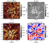 |
Fig. 2. Region-of-interest maps of Hα − 1.5 Å intensity, vertical field in the photosphere, Bz, source function, S0, and the Doppler velocity, v0, at the reference time. |
The maps of the parameters as well as monochromatic intensity data constructed from the different raster scans have been spatially aligned to yield a set of three-dimensional data cubes. The spatial alignment of the data from each scan has been done successively by spatially correlating the Hα − 1.5 Å image and the one of its reference scan, which is either its previous scan or its next scan, with the image rotation caused by the Earth’s rotation being taken into account. The first reference is set to the scan in the middle of the observation. We used the Hα − 1.5 Å images for alignment because these images clearly display network bright points that correspond to strong magnetic concentrations. Once the alignment is done, the velocity time variation at a fixed point can be obtained from the velocity data cube.
We analyzed the time variation in the Doppler velocity at each point based on the Morlet wavelet analysis following Torrence & Compo (1998). First of all, we subtracted the first-order polynomial fit from the velocity data to obtain the trend-subtracted velocity, vn, at discrete times indexed by n that are equally spaced. The two-dimensional wavelet transform, Wnj, was then calculated from vn at discrete times, tn, indexed by n as well as at discrete periods, Tj, indexed by j, where the logarithms of period are equally spaced. We defined the wavelet power, Pnj ≡ C|Wnj|2/Tj, at a period, Tj (in units of km2 s−2), by introducing a numeric factor, C (see Eq. (14) of Torrence & Compo 1998), to ensure the condition that the dispersion of velocity oscillation, σ2, is equal to the summation of  over the same range of j as in
 (1)
(1)
Here  is the time-averaged power of velocity specified by the formula
 (2)
(2)
where n1 and n2 refer, respectively, to the indexes of the first and last instants at the specified j inside the cone of influence. As the magnitude of Pnj depends on the bin size of log T, it would be better to work with (dP/dlog T)nj defined as
 (3)
(3)
in terms of the bin size, Δlog T ≡ log Tn + 1 − log Tn, which is taken to be constant.
3. Results
3.1. Chromospheric rosette and photospheric bright points
The rosette in which we are interested is well identified from the Hα monochromatic images of the observed region constructed from the reference raster scan as given in Fig. 1. The rosette consists of two regions: a central region that displays either bright or dark clumps in Hα + 0.0 Å, and a fibril region that surrounds the central region and displays a number of fibrils visible in Hα ± 0.5 Å.
The central region seen in Hα − 1.5 Å, as is shown in Figs. 1 and 2, contains a cluster of bright points that are more or less randomly scattered. These points correspond to magnetic flux concentrations of positive polarity that are identified in the Bz map. From Fig. 2, we find it very difficult to spatially relate the fine-scale structures of the chromospheric rosette seen in the maps of S0 and v0 of the Hα line to the photospheric bright points seen in the map of −1.5 Å intensity. Moreover, we found from the NIRIS data that vector magnetic fields are vertical at the center of every magnetic concentration. Therefore, the photospheric magnetic fields underlying the Hα rosette represent a cluster of magnetic flux concentrations, each of which can be identified with a vertical flux tube. As a matter of fact, the rosette appears as an organized chromospheric structure, whereas the bright points are not organized except for their clustering. We estimate the total magnetic flux of all the magnetic concentrations of positive polarity in this cluster to be 7 × 10¹⁹ Mx.
The map of v0 in Fig. 2 clearly indicates that the Doppler velocity also oscillates with position, especially in the radial direction from the center. This oscillatory spatial pattern supports our interpretation that the temporal velocity oscillations at fixed points to be described below represent MHD waves that propagate along magnetic fields in the rosette.
3.2. Velocity oscillations at selected points
Figure 3 presents the time variation in velocity at four selected positions, hereafter Point 1, Point 2, Point 3, and Point 4. The time-averaged power spectra at these positions are given in Fig. 4. It is clear from this figure that the properties of velocity oscillation significantly vary from position to position in this rosette. We find a number of oscillations with periods ranging from 2 min to 16 min, some of which often appear together, being superposed.
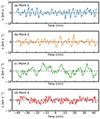 |
Fig. 3. Time variation in velocity at each selected point. |
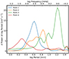 |
Fig. 4. Time-averaged wavelet power spectra, |

Point 1 and Point 2 are located inside the central region of the rosette (see Figs. 1 and 2). The velocity variations at these two points are dominated by oscillations of periods < 8 min. Point 1 represents a position other than bright points in the central region of the rosette. The total power at this point is 4.8 km2 s−2. Its velocity variation is fairly simple, in that the time-averaged wavelet power is singly peaked at 4.1 min. We conjecture this value may be close to the acoustic cutoff period at this point.
Point 2 represents a position inside a bright point in the central region of the rosette. As this bright point moves around with the shape gradually changing with time, we have examined the time variation in velocity in two ways: first, by tracing the feature (bright point) at the location at the reference time both forward and backward, using the nonlinear affine velocity estimator (NAVE) technique of optical flow tracking (Chae & Moon 2009), and second, by fixing the location without feature tracking. We find that the two velocity variations differ a little from each other, especially at times much earlier or later than the reference time, but there is no significant difference in the oscillation characteristics between the two. Hence, we present only the second results obtained by fixing the location of velocity sampling. It can be seen from the figure that, even though it has a slightly smaller total power of 4.2 km2 s−2 than at Point 1, the variation in velocity at this point is more complex, with the time-averaged power displaying three peaks at 3.1 min, 4.8 min, and 6.9 min, respectively.
Point 3 represents the inner part of the fibril region of the rosette. The velocity variation at this point has a total power of 7.7 km2 s−2, dominated by long-period oscillations. The time-averaged power spectrum peaks at the periods of 5.8 min, 9.7 min, and 16.5 min, with the strongest power occurring at periods of about 16.5 min. These oscillations correspond to the long-period network oscillations first reported by Lites et al. (1993).
Point 4 is located at the outermost part of the fibril region. The velocity fluctuation at this point has a total power of 3.1 km2 s−2. It is very different from that at Point 3, even though both these points are located in the fibril region. Unlike Point 3, it lacks significant-power oscillations of periods > 5 min, and instead displays short-period oscillations that peak at a period of 2.0 min. This period is the shortest among the peak-power periods we found at the four points.
The wavelet power spectra in Fig. 5 indicate that each velocity oscillation lasts for a finite duration. Furthermore, we find that there is a correlation between the oscillation period, T, and the duration, τ; shorter-period oscillations last for shorter durations and longer-period oscillations last for longer durations. For instance, we find an oscillation packet of T = 4 min at Point 1 lasting for τ = 17 min around time t = −9 min, one of T = 3.1 min at Point 2 lasting for τ = 13 min around t = −14 min, one of T = 16 min at Point 3 lasting for τ = 50 min around time t = −10 min, and one of T = 2 min period at Point 4 lasting for τ = 8 min around t = 6 min. Based on these examples, we obtain a rule of thumb: τ/T ≃ 4, which holds between the duration and period.
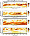 |
Fig. 5. Time-dependent wavelet power spectra at the four points. |
3.3. Spatial distribution of velocity oscillation power
The power maps in Fig. 6 indicate that the spatial distribution of oscillation power depends on the frequency or period. The oscillation power at each band is non-uniformly distributed over the region of interest in two different ways. First, there exist small-scale inhomogeneities of powers that appear clumpy in the central region and filamentary in the fibril region. Second, there is a slowly varying (or azimuthally averaged) pattern of power that depends on the radial distance from the center of the rosette. This pattern changes from band to band.
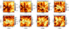 |
Fig. 6. Maps of time-averaged oscillation power summed over the different bands. |
We find from the figure that the oscillations at periods of 1−2 min (16−8 mHz) have significant power in the outermost parts of the fibril region, whereas they are negligibly weak in the central region as well as in the inner parts of the fibril region. The power of the oscillations in the outermost parts appear the strongest at periods around 2.0 min.
At periods 2−2.8 min (frequencies 8−6 mHz), the oscillation powers become strong not only in the outermost parts of the fibril region, but also in the central region. The oscillation power in this band is weak in the inner parts of the fibril region surrounding the central region. This suppression of oscillation power around the network, dubbed a magnetic shadow, was first known from the FUV line and continuum observations (Judge et al. 2001; McIntosh & Judge 2001) and was later identified from the Ca II 854.2 nm line observations as well (Vecchio et al. 2007).
At periods of 2.8−4.0 min (6−4 mHz), the oscillations in the central region become much stronger than those in the outermost parts of the fibril region. The enhanced oscillation powers in the central region occur in clumps with a typical size of 2.5″ (1800 km) and a typical band-integrated power of 1.5 km2 s−2. At periods of 4.0−5.7 min (4−3 mHz), the oscillation powers are strong at the boundary between the central region and the fibril region. At this boundary, oscillation powers are concentrated in clumps showing tails elongated into the fibril region. This indicates the propagation of the oscillations along the magnetic fields inclined from the vertical.
At periods of 5.7−8.0 min, the structures of enhanced oscillation powers become longer than at shorter periods. They extend further into the fibril region. As a result, the oscillation powers in the fibril region become comparable to those in the central region. At longer periods of > 8.0 min, the oscillation powers are strong in the fibril region, and become weak in the central region. There is a tendency for longer-period oscillation powers to occur in more extended structures in the fibril region. These long-period (> 8 min) oscillations in the fibril region are usually stronger than the short-period (< 8 min) oscillations in the central region. These long-period oscillations reach peaks in the fibril region at some distances from the central region and become weaker at farther distances.
The properties of the oscillations in this rosette may be summarized in terms of the total power and power-averaged period given in Fig. 7. We find from the figure that the total power of oscillations is non-uniformly distributed, ranging from 2 to 8 km2 s−2 in the central region and from 5 to 20 km2 s−2 in the fibril region. The peak-power periods are also non-uniformly distributed, ranging from 4 to 6 min in the central region, and from 6 to 20 min in the fibril region. The oscillations with the shortest peak period of about 2 min are found in the outermost parts of the fibril region, with a typical total power of 2.5 km2 s−2.
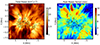 |
Fig. 7. Maps of power-averaged period obtained from the observation. |
4. Discussion
4.1. Three groups of oscillations
We find that the oscillations with periods in a wide range from 2 to 16 min occur in the rosette. From only the four selected points, we have identified oscillations with periods of 2.0 min, 3.1 min, 4.1 min, 4.8 min, 5.8 min, 6.9 min, 9.7 min, and 16.5 min, illustrating that the oscillation periods are diverse. This result is compatible with the previous studies on the network oscillations that reported diverse periods (e.g., Lites et al. 1993; Banerjee et al. 2001; Sadeghi & Tavabi 2022).
The observed oscillations with periods in a wide range can be categorized into three groups depending on the occurrence location and the period range. This categorization is simply for the convenience of phenomenological description. We do not insist that different groups be physically distinct. Group I oscillations occur in the central region and have periods in the range from 3 to 6 min. Group I oscillations are similar to umbral oscillations as the central region is similar to a sunspot umbra. Group II oscillations occur in the fibril region and have periods in the range from 6 to 20 min. These oscillations are similar to the oscillations of running waves observed in a sunspot penumbra and superpenumbra. Finally, group III oscillations are high-frequency oscillations with periods shorter than 3 min that occur in the outermost part of the fibril region. This kind of oscillation is not similar to any of the oscillations observed in sunspots.
These oscillations of diverse periods in the chromospheric network rosette likely represent MHD waves, including longitudinal waves that oscillate in the direction of the magnetic field and transverse waves that oscillate in the direction perpendicular to the magnetic field. In this regard, we note the study by Kwak et al. (2023, hereafter KW) on the detection of transverse waves. KW used the same data set that we use, in order to identify transverse waves in the outermost parts of the fibril region where magnetic fields are supposedly predominantly horizontal. However, much of the searched area is outside our region of interest. KW identified transverse waves with periods broadly ranging from 1.5 to 30 min. This range is comparable to the range of the oscillation periods we found. This suggests the possibility that some, if not all, of the oscillations we observed may represent transverse waves.
4.2. Group I oscillations
If these oscillations represent longitudinal MHD waves, the most important parameter determining these periods is the acoustic cutoff period in the atmosphere. It has been well known that the cutoff frequency plays the role of the natural frequency of an isothermal atmosphere that displays a resonance-like behavior when the atmosphere is perturbed (Lamb 1932; Fleck & Schmitz 1991; Kalkofen et al. 1994; Chae & Goode 2015). In a non-isothermal atmosphere, the acoustic cutoff period is determined by its minimum temperature (Chae & Litvinenko 2018). Moreover, the peak-power frequency of oscillations driven in the photosphere and below is shown to be very close to this acoustic frequency (Chae et al. 2019).
From Eq. (68) of Chae et al. (2019), we obtain the relationship in the solar atmosphere,
 (4)
(4)
where k is a numeric factor that relates the peak-power frequency and the cutoff frequency and θ is the propagation direction of the longitudinal oscillations, which is set to zero in the field-free region and to the inclination of magnetic fields from the vertical in strong-field regions. With the fixed values of k = 1.05, γ = 1.67, and μ = 1.25, we find that the peak frequency, νp, is determined by the minimum temperature, Tm, and the field inclination, θ. If we choose Tm = 4700 K, the mean minimum temperature of the network atmosphere (Fontenla et al. 1993) and θ = 0, we obtain νp = 5.3 mHz, corresponding to the period of 3.1 min. This is comparable to the shortest period found in group I oscillations. Therefore, we believe that the periods of group I oscillations are strongly related to the acoustic cutoff in the atmosphere.
Most periods of group I oscillations, however, range from 4 to 6 min, and are longer than the above value of 3.1 min. This deviation may be explained in terms of other physical factors. The most important factor may be the magnetic field inclination. If fields are more inclined from the vertical, the acoustic cutoff period gets longer, which was considered important in the p-mode driving of spicules (e.g., De Pontieu et al. 2004) and was later confirmed from MHD simulations (Heggland et al. 2011). If the periods from 4.0 to 6 min in group I oscillations are to be attributed to the inclination effect only, the inclination, θ, should range from 40 to 60°. The inclination in this range may be found in the outer parts of each photospheric magnetic concentration. However, it is unclear whether the inclination of photospheric fields is the same as that in the temperature minimum level. The effect of flux tube expansion with height may have to be considered for a reasonable picture.
Another factor that may have to be taken into account is the breakdown of the assumptions implicit in Eq. (4). It is assumed that the oscillations represent acoustic waves guided through a rigid magnetic flux tube with a uniform cross section. This assumption holds best in a sunspot umbra where magnetic fields are strong enough, but may break down in network magnetic fields that may be neither strong enough to be rigid nor uniform with height. This aspect would have to be investigated, even though the analytical study of Roberts (2019) indicates that the cutoff frequency of slow MHD waves in an isolated thin flux tube deviates from the acoustic cutoff frequency by only a few percentage points.
4.3. Group II oscillations
The periods of group II oscillations, from 6 to 20 min, are even longer than those of group I oscillations. If these long-period oscillations represent longitudinal waves and the periods are to be explained in terms of inclination, magnetic fields should have an inclination as large as 80°. This explanation is simple, but has the problem that the total power of the longitudinal oscillations should be much stronger than the observed total power of 5 to 20 km2 s−2. Therefore, the long periods may not be from the large inclination, or the group II oscillations may not represent longitudinal waves.
If the group II oscillations do represent longitudinal waves, we can propose an alternate explanation for the long periods: the merging of longitudinal shock waves (Chae et al. 2014, 2015). This process occurs after a train of sinusoidal waves nonlinearly develop into a train of shock wave fronts. Often a preceding shock front is caught by the following shock front. This merging of two shock fronts leads to the lengthening of the interval between two successive ones, corresponding to the increase in period. This may be the origin of the long-period oscillations observed in the fibril region. We also note that, even without shock merging, the successive impinge on the upper chromosphere by a series of shock waves may lead to a ballistic trajectory characterized by a longer timescale, as in the rebound shock model first proposed by Hollweg (1982).
If the group II oscillations do not represent longitudinal waves but transverse waves such as kink waves, we can think of a different explanation: the effect of photospheric resonance of kink waves associated with the cutoff in a non-isothermal atmosphere (Chae et al. 2022). It was known from the study of Lopin et al. (2014) that kink waves are not subject to cutoff in an isothermal atmosphere, which went against earlier theoretical studies (e.g., Hasan & Kalkofen 1999) based on the thin flux tube equations derived by Spruit (1981). In a non-isothermal atmosphere, however, kink waves are subject to cutoff. Lopin & Nagorny (2017) estimated the cutoff period of kink waves in the quiet Sun at 700 s, which is quite within the range of the periods of group II oscillations.
Our observations indicate that if the group II oscillations do represent transverse waves, these waves must be significantly polarized in the vertical direction; that is, velocity oscillates in the vertical direction with significant amplitudes. On the other hand, transverse waves that are significantly polarized in the horizontal direction can be detected from the imaging observations by tracking transverse motions of individual fibrils on the plane of the sky. As a matter of fact, such transverse waves were detected in network fibrils by Kuridze et al. (2012, 2013). These transverse waves are characterized by periods ranging from 70 to 280 s, with the most frequent occurrence at 165 s. These periods overlap the ones of the group II oscillations only slightly, whereas they significantly overlap the ones of group I oscillations. This comparison suggests the possibility that some of the group I oscillations may also represent transverse waves, and future imaging observations may reveal horizontally polarized transverse waves of longer periods that are compatible with the group II oscillations.
4.4. Group III oscillations
We have identified group III oscillations with the 3-min transverse waves reported by KW. As a consequence, it follows that group III oscillations represent transverse waves such as kink waves in the significantly horizontal parts of the magnetic canopy supported by the rosette, as is described above. We believe these oscillations may be excited by the collision of shock waves in the sub-canopy domain and the canopy, as in the schematic picture presented by Wedemeyer-Böhm et al. (2009). These shock waves may develop from 3-min oscillations in the sub-canopy domain (internetwork regions) below the canopy. Note that the non-linear steepening of oscillations leads to the production of second harmonic and higher-order harmonics (Chae & Litvinenko 2017), which may explain the occurrence of oscillations with periods shorter than 3 min.
4.5. The rosette and sunspots: Similarities and differences
The Hα network rosette in which we are interested is similar to a small sunspot in that it appears as an organized structure consisting of a central region that looks like the umbral region of the sunspot and a fibril region that looks like the penumbral (or superpenumbral region) of the sunspot. The estimated magnetic flux of the rosette, 7 × 10¹⁹ Mx, is comparable to that of a small pore in an active region (Zwaan 1987), and about 10 times the minimum amount of flux required for a tiny pore to be formed (Cho et al. 2010).
Note that the oscillations in the rosette are also similar to oscillations in a sunspot in their dominant periods and their preferred locations. In a sunspot, 3-min oscillations occur in the umbra, 5-min oscillations in the penumbra, and long-period (> 10 min) oscillations in the superpenumbra (see, e.g., Chae et al. 2014). Our group I oscillations in the rosette are similar to the 3-min oscillations in sunspots, and the group II oscillations in the rosette are similar to the 5-min oscillations or long-period oscillations in sunspots.
Despite the overall similarity, there also exist many differences in the oscillation characteristics between the rosette and a sunspot. The velocity variation at a particular point in the rosette is more complex than at a particular point in a sunspot. It usually comprises oscillations with multiple periods, whereas the oscillations of a single period dominate at a particular point inside a sunspot. Moreover, the spatial distribution of oscillation power in a rosette displays inhomogeneities that appear clumpy in the central region and filamentary in the fibril region, which is not surprising at all, considering the inhomogeneous nature of the photospheric magnetic fields underlying the rosette.
As a matter of fact, there is a fundamental difference in the plasma β distribution between a rosette and a small sunspot. Note that the β = 1 surface is very important in characterizing oscillations and waves. In a sunspot, the β = 1 surface is located in the photospheric level inside it (e.g., Mathew et al. 2004; Cho et al. 2017), in the interface between it and the surrounding neighboring field-free region in the lower atmosphere, and in the lower boundary of the canopy structures extended far from it in the upper atmosphere. In the atmosphere of a sunspot umbra, it holds β ≪ 1, so that slow MHD waves, for example, may be approximated as guided acoustic waves.
This kind of simple approach may not be applicable straightforwardly to the study of Doppler velocity oscillations in the rosette. In the rosette, the β = 1 surface is much more complex than that in a sunspot. A two-dimensional picture of the β = 1 surface in a quiet region provided by Wedemeyer-Böhm et al. (2009) gives us a good insight into this aspect. It is very likely that at the photospheric level, β > 1 at most points, and β < 1 only inside strong magnetic field concentrations. In the lower chromosphere, the fraction of β < 1 points increases. Above a particular level in the upper atmosphere, all the points inside the rosette satisfy β < 1, and this is probably also the case in the atmospheric level of the Hα core formation. The β = 1 surface of the rosette should be considered in the three-dimensional space, which may be much more complex than the two-dimensional picture. Because of the complexity of the β = 1 surfaces, it will be difficult, therefore, to properly characterize the Hα Doppler velocity oscillations in a network rosette in relation to photospheric oscillations, unlike in sunspot oscillations.
5. Conclusion
We have categorized the Doppler velocity oscillations observed in the Hα rosette into three groups: group I oscillations with periods from 3 to 6 min in the central region, group II oscillations with longer periods from 6 to 20 min in the fibril region, and group III oscillation with periods shorter than 3 min in the outermost part of the fibril region. We conjecture that the group I oscillations may represent primarily longitudinal MHD waves in vertical or moderately inclined magnetic fields, and the group II oscillations primarily transverse MHD waves in inclined magnetic fields. Finally, the group III oscillations may be transverse MHD waves in the predominantly horizontal magnetic fields of the magnetic canopy supported by the network. The full physical interpretation of the observed oscillations in terms of MHD waves has to wait for knowledge of spatial variation in the oscillation phase, which is beyond the scope of this study.
The rosette we examined looks similar to a small sunspot in its morphology and oscillation properties, but there are differences as well. In particular, the magnetic fields guiding longitudinal waves and transverse waves are neither uniform nor rigid in the photosphere and chromosphere, unlike in a sunspot. It is worth further investigating oscillations and waves in a network rosette in comparison with those in a sunspot.
Acknowledgments
This research was supported by the National Research Foundation of Korea (RS-2023-00208117). J. Kang was supported by the National Research Foundation of Korea (RS-2023-00273679). E.-K. Lim was supported by the Korea Astronomy and Space Science Institute under the R&D program of the Korean government (MSIT; No. 2025-1-850-02). M.M. acknowledges the support of the Brain Pool program funded by the Ministry of Science and ICT through the National Research Foundation of Korea (RS-2024-00408396) and DFG grant WI 3211/8-2, project number 452856778. BBSO operation is supported by US NSF AGS 2309939 grant and the New Jersey Institute of Technology. The GST operation is partly supported by the Korea Astronomy and Space Science Institute and the Seoul National University.
References
- Banerjee, D., O’Shea, E., Doyle, J. G., & Goossens, M. 2001, A&A, 371, 1137 [NASA ADS] [CrossRef] [EDP Sciences] [Google Scholar]
- Beckers, J. M., & Tallant, P. E. 1969, Sol. Phys., 7, 351 [NASA ADS] [CrossRef] [Google Scholar]
- Chae, J., & Goode, P. R. 2015, ApJ, 808, 118 [NASA ADS] [CrossRef] [Google Scholar]
- Chae, J., & Litvinenko, Y. E. 2017, ApJ, 844, 129 [Google Scholar]
- Chae, J., & Litvinenko, Y. E. 2018, ApJ, 869, 36 [NASA ADS] [CrossRef] [Google Scholar]
- Chae, J.-C., & Moon, Y.-J. 2009, JKAS, 42, 61 [Google Scholar]
- Chae, J., Park, H.-M., Ahn, K., et al. 2013, Sol. Phys., 288, 1 [NASA ADS] [CrossRef] [Google Scholar]
- Chae, J., Yang, H., Park, H., et al. 2014, ApJ, 789, 108 [NASA ADS] [CrossRef] [Google Scholar]
- Chae, J., Song, D., Seo, M., et al. 2015, ApJ, 805, L21 [NASA ADS] [CrossRef] [Google Scholar]
- Chae, J., Kang, J., & Litvinenko, Y. E. 2019, ApJ, 883, 72 [Google Scholar]
- Chae, J., Madjarska, M. S., Kwak, H., & Cho, K. 2020, A&A, 640, A45 [NASA ADS] [CrossRef] [EDP Sciences] [Google Scholar]
- Chae, J., Cho, K., Kang, J., et al. 2021, JKAS, 54, 139 [Google Scholar]
- Chae, J., Cho, K., Lim, E.-K., & Kang, J. 2022, ApJ, 933, 108 [CrossRef] [Google Scholar]
- Cho, K.-S., Bong, S.-C., Chae, J., Kim, Y.-H., & Park, Y.-D. 2010, ApJ, 723, 440 [Google Scholar]
- Cho, I. H., Cho, K. S., Bong, S. C., et al. 2017, ApJ, 837, L11 [Google Scholar]
- De Pontieu, B., Erdélyi, R., & James, S. P. 2004, Nature, 430, 536 [Google Scholar]
- Dunn, R. B., & Zirker, J. B. 1973, Sol. Phys., 33, 281 [NASA ADS] [Google Scholar]
- Fleck, B., & Schmitz, F. 1991, A&A, 250, 235 [NASA ADS] [Google Scholar]
- Fontenla, J. M., Avrett, E. H., & Loeser, R. 1993, ApJ, 406, 319 [Google Scholar]
- Giovanelli, R. G. 1972, Sol. Phys., 27, 71 [NASA ADS] [CrossRef] [Google Scholar]
- Hasan, S. S., & Kalkofen, W. 1999, ApJ, 519, 899 [NASA ADS] [CrossRef] [Google Scholar]
- Heggland, L., Hansteen, V. H., De Pontieu, B., & Carlsson, M. 2011, ApJ, 743, 142 [CrossRef] [Google Scholar]
- Hollweg, J. V. 1982, ApJ, 257, 345 [NASA ADS] [CrossRef] [Google Scholar]
- Jess, D. B., Reznikova, V. E., Van Doorsselaere, T., Keys, P. H., & Mackay, D. H. 2013, ApJ, 779, 168 [Google Scholar]
- Judge, P. G., Tarbell, T. D., & Wilhelm, K. 2001, ApJ, 554, 424 [Google Scholar]
- Kalkofen, W., Rossi, P., Bodo, G., & Massaglia, S. 1994, A&A, 284, 976 [Google Scholar]
- Kontogiannis, I., Tsiropoula, G., & Tziotziou, K. 2010a, A&A, 510, A41 [NASA ADS] [CrossRef] [EDP Sciences] [Google Scholar]
- Kontogiannis, I., Tsiropoula, G., Tziotziou, K., & Georgoulis, M. K. 2010b, A&A, 524, A12 [NASA ADS] [CrossRef] [EDP Sciences] [Google Scholar]
- Kuridze, D., Morton, R. J., Erdélyi, R., et al. 2012, ApJ, 750, 51 [NASA ADS] [CrossRef] [Google Scholar]
- Kuridze, D., Verth, G., Mathioudakis, M., et al. 2013, ApJ, 779, 82 [NASA ADS] [CrossRef] [Google Scholar]
- Kwak, H., Chae, J., Lim, E.-K., et al. 2023, ApJ, 958, 131 [NASA ADS] [CrossRef] [Google Scholar]
- Lamb, H. 1932, Hydrodynamics (Cambridge: Cambridge University Press) [Google Scholar]
- Lee, K.-S., Chae, J., Park, E., et al. 2022, ApJ, 940, 147 [Google Scholar]
- Lim, E.-K., Chae, J., Cho, K., et al. 2025, ApJ, 981, 185 [Google Scholar]
- Lites, B. W., Rutten, R. J., & Kalkofen, W. 1993, ApJ, 414, 345 [Google Scholar]
- Lopin, I., & Nagorny, I. 2017, ApJ, 840, 26 [Google Scholar]
- Lopin, I. P., Nagorny, I. G., & Nippolainen, E. 2014, Sol. Phys., 289, 3033 [NASA ADS] [CrossRef] [Google Scholar]
- Mathew, S. K., Solanki, S. K., Lagg, A., et al. 2004, A&A, 422, 693 [NASA ADS] [CrossRef] [EDP Sciences] [Google Scholar]
- Maurya, R. A., Chae, J., Park, H., et al. 2013, Sol. Phys., 288, 73 [Google Scholar]
- McIntosh, S. W., & Judge, P. G. 2001, ApJ, 561, 420 [Google Scholar]
- Mehltretter, J. P. 1974, Sol. Phys., 38, 43 [CrossRef] [Google Scholar]
- Roberts, B. 2019, MHD Waves in the Solar Atmosphere (Cambridge: Cambridge University Press) [Google Scholar]
- Sadeghi, R., & Tavabi, E. 2022, MNRAS, 512, 4164 [Google Scholar]
- Spruit, H. C. 1981, A&A, 98, 155 [NASA ADS] [Google Scholar]
- Sych, R., & Altyntsev, A. 2023, MNRAS, 519, 4397 [Google Scholar]
- Sych, R., Zhu, X., Chen, Y., & Yan, F. 2024, MNRAS, 529, 967 [Google Scholar]
- Torrence, C., & Compo, G. P. 1998, Bull. Am. Meteorol. Soc., 79, 61 [Google Scholar]
- Tsiropoula, G., Tziotziou, K., Kontogiannis, I., et al. 2012, Space Sci. Rev., 169, 181 [Google Scholar]
- Vecchio, A., Cauzzi, G., Reardon, K. P., Janssen, K., & Rimmele, T. 2007, A&A, 461, L1 [CrossRef] [EDP Sciences] [Google Scholar]
- Wedemeyer-Böhm, S., Lagg, A., & Nordlund, Å. 2009, Space Sci. Rev., 144, 317 [Google Scholar]
- Zirin, H., & Stein, A. 1972, ApJ, 178, L85 [NASA ADS] [CrossRef] [Google Scholar]
- Zwaan, C. 1987, ARA&A, 25, 83 [NASA ADS] [CrossRef] [Google Scholar]
All Figures
|
Fig. 1. Monochromatic images constructed from the reference raster (17:28:37 UT) at several wavelengths. The field of view is 32″ by 41″ and the spatial sampling size of 0.16″ is in each direction. The red squares indicate the region of interest, and the symbols mark the four positions selected to illustrate the time variation in the Doppler velocity and its wavelet analysis. |
| In the text | |
|
Fig. 2. Region-of-interest maps of Hα − 1.5 Å intensity, vertical field in the photosphere, Bz, source function, S0, and the Doppler velocity, v0, at the reference time. |
| In the text | |
|
Fig. 3. Time variation in velocity at each selected point. |
| In the text | |
|
Fig. 4. Time-averaged wavelet power spectra, |
| In the text | |
|
Fig. 5. Time-dependent wavelet power spectra at the four points. |
| In the text | |
|
Fig. 6. Maps of time-averaged oscillation power summed over the different bands. |
| In the text | |
|
Fig. 7. Maps of power-averaged period obtained from the observation. |
| In the text | |
Current usage metrics show cumulative count of Article Views (full-text article views including HTML views, PDF and ePub downloads, according to the available data) and Abstracts Views on Vision4Press platform.
Data correspond to usage on the plateform after 2015. The current usage metrics is available 48-96 hours after online publication and is updated daily on week days.
Initial download of the metrics may take a while.